Optimal Component Sizing for Peak Shaving in Battery Energy Storage System for Industrial Applications

Abstract

Recent attention to industrial peak shaving applications sparked an increased interest in battery energy storage. Batteries provide a fast and high power capability, making them an ideal solution for this task. This work proposes a general framework for sizing of battery energy storage system (BESS) in peak shaving applications. A cost-optimal sizing of the battery and power electronics is derived using linear programming based on local demand and billing scheme. A case study conducted with real-world industrial profiles shows the applicability of the approach as well as the return on investment dependence on the load profile. At the same time, the power flow optimization reveals the best storage operation patterns considering a trade-off between energy purchase, peak-power tariff, and battery aging. This underlines the need for a general mathematical optimization approach to efficiently tackle the challenge of peak shaving using an energy storage system. The case study also compares the applicability of yearly and monthly billing schemes, where the highest load of the year/month is the base for the price per kW. The results demonstrate that batteries in peak shaving applications can shorten the payback period when used for large industrial loads. They also show the impacts of peak shaving variation on the return of investment and battery aging of the system.

1. Introduction

In power systems, the load profile can be characterized by the “peak load times” of the system—short periods of time when large amounts of power are required [1]. The peak load periods can occur at different times during the day, depending on the season of the year and the load composition (residential, commercial, or industrial). Peaks of demand impact the network planning because the electrical infrastructure of transmission and distribution systems must be designed to support the maximal demand of the system [2]. For this reason, the electrical power grid infrastructure may be underutilized most of the time, reaching its loading capacity limit at only a few moments of the year. Consequently, commercial and industrial customers are charged not only by their total energy consumption but also by their highest power demand that dominates the grid construction costs. The electricity charge can be discriminated in subcomponents like the generation cost, taxes, and fees which represent a small portion of the total electricity payment of the customers. Accordingly, commercial and industrial customers are interested in decreasing energy and power costs, which are the most significant part of the total charges, without lowering their energy consumption. In this context, energy storage systems (ESS) can be used to help customers flatten their demand profile by storing energy during off-peak periods and releasing it during peak load periods.

The deployment of ESS can achieve another benefit besides the reduction of demand charges for customers. For instance, system operators can reduce the need of network reinforcement by sizing the infrastructure for a more flat profile coupled with ESS, instead of designing it for the highest power demand [3]. Depending on the market conditions, other benefits can be achieved. The customers can take advantage of time of use energy price [4] by discharging the ESS when the energy price at the peak load periods is more expensive than the price during the off-peak periods. This can lead to additional electricity bill reduction [5].

Energy storage system technologies are used for a variety of applications [6,7]. They can be classified in many different ways, according to the application area [8], based on the energy conversion [9], or depending on the quantity of energy that the ESS can provide [10]. For “power-type” applications like peak shaving, the ESS have to maintain a constant delivery of power [11].

Although the improvements of battery energy storage system (BESS) efficiency and life cycle are increasing the interest for this type of storage [12], the high investment costs necessary for BESS solutions still raise concerns about the economic viability of this technology in power system applications [13,14,15,16]. Therefore, an important aspect of the deployment of any BESS project is their proper power and energy sizing [17]. If a BESS is not sized properly, it can generate negative results from an economic perspective. While small BESS may result in excessive aging-related depreciation cost, over-sizing systems may not attain optimal cost-benefit ratio due to their relatively high initial investment cost.

In response to the need to properly size BEES, several studies aiming to find the optimal sizing of BESS have been conducted [6]. Recent work by Merei et al. [18] concentrates on commercial applications of BESS. The authors use sensitivity analysis to study the maximization of energy self-consumption via storage integration. The techno-economic analysis reveals that, for most commercial applications, BESS is not favored economically when battery degradation is taken into account. Other previous work by Magnor and Sauer [19] and Merei et al. [20] analyzed the optimal sizing of storage in the context of island grids and home storage systems. The authors propose a genetic algorithm-based method to model a non-linear set of equations including battery-aging characteristics. However, the solver results may not find a globally optimal solution to the described problem, and the studies do not provide design rules for future storage systems.

A sophisticated optimization method applied to find the best-suited battery storage system located in a residential suburban area has been described by Tant et al. [21]. A multi-objective function is used to find the balance between voltage regulation, peak power reduction, and annual cost. A grid operator can use this method to support the decision of temporarily installing a BESS in problematic feeders to postpone grid upgrades in the short term due to work planning issues. By comparing the cost of grid upgrades, the grid operator may conclude that the BESS is also a valuable alternative in the long term. Recent work by Rahmann et al. [1] proposed an approach to determine the break-even points for different BESS considering a wide range of life cycles, efficiency, energy price, and power price. The results presented in this work show that depending on the values of round trip efficiency, life cycles, and power price, there are BESS technologies that are already profitable when considering only peak shaving applications. Although the authors model an optimization algorithm used for the sizing of the storage system, only the distribution company perspective is considered.

In contrast to the important contributions mentioned above, this work proposes a linear optimization method to define a cost-optimal sizing of the battery and power electronics for peak shaving application in industrial settings. In addition, this paper also presents a case study conducted with real industrial profiles, a techno-economic analysis evaluating the return on investment (ROI) of the system and battery degradation, and a linear programming (LP) approach allowing exact solution determination for BESS sizing. At the same time, the power flow optimization reveals the best storage operation considering energy purchase, peaks of consumption, and battery aging.

The remainder of this paper is organized as follows: Section 2 introduces the system layout, parameters necessary as input for the subsequent optimization procedure, and the aging model. The concepts of LP methodology, including equations and constraints for optimization, and a case study where different industrial profiles verify effectiveness of the proposed model are presented in Section 3. Finally, Section 4 provides the conclusion and outlines possible directions for future research.

2. System Layout and Storage Model

2.1. System Layout

The energy management system proposed in this study is derived from measured and simulated data for an exemplary BESS. The simulations involve a grid-connected system shown in a schematic diagram in Figure 1a. The arrows in this figure illustrate the power flow direction for all component links. Additionally, Figure 1b illustrates all price components for industrial customers: the total energy consumption ${\mathrm{E}}_{\mathrm{total}}=\sum {\mathrm{load}}_i$ where i denotes an averaged time segment of 15 min, the maximum power peak in the billing period $P_{\max }$, and the maximum power peak after peak shave $P_{\mathrm{PS}}$. Other variables necessary for subsequent modeling are explained in more detail later, along with the optimization problem definition.

2.2. Economic and Legal Framework for Industrial Customers

BESS are very flexible devices that can be used for many different applications [6]. Depending on the application, several factors influence the attractiveness for energy storage systems. Particularly in behind-the-meter-scenarios (BTM), the economic attractiveness of energy storage systems depends not so much on the electricity price itself, but on the pricing structure [22].

Peak shaving is a typical BTM application that concentrates on the reduction of the peak demand of consumers. Peak shaving systems are only attractive in markets where demand charges amount to a proportionally large part of the electricity price. Already at a very early stage of electricity system development, system operators introduced electricity tariffs that included a demand based part added to the usage based part of electricity costs [23]. This scheme has been established to provide an incentive for efficient grid usage. This is a so-called cost reflective tariff, since the level of demand is the main driver of network costs (i.e., grid reinforcement and transformer overloading) [24].

Battery storage is still a new technology associated with high perceived investment risk. This is likely the reason why most storage projects are currently conducted in well-developed countries [25]. According to a study by Azure International, the most attractive countries for demand charge management in the commercial and industrial (C&I) sector are Australia, France, the USA (California), Japan and Germany.

Electricity costs are paid via the utility company selected by the consumer. The utility company keeps a small percentage for itself to cover generation and retail costs. Also, it transfers taxes, fees and surcharges to the relevant authorities and transfers network costs to the system operator responsible for the corresponding system. Therefore, the location of the network connection point defines network costs. For instance, the two eastern transmission system operators (TSOs) in Germany charge significantly higher prices than the two western TSOs, but prices also differ from one distribution system operator to the next inside the same regulation zone. Specifically, commercial and industrial customers who (typically) exceed 100.000 kWh energy consumption per year or 500 kW of average power demand pay an additional power price per kW to the energy price per kWh. The electricity price in the C&I sector typically has the following components:

• Electricity generation (wholesale prices and retail costs); prices depend on negotiations between customer and utility company.
• The network costs (transmission and distribution) are subdivided into two categories. First, power price per kilowatt, based on the maximum power peak in the billing period; this is the only power-specific price component; prices vary with connected voltage level, billing period, distribution system operator and duration factor. Second, energy price per kilowatt hour, based on the total energy consumption.
• The total for standard rates including taxes, fees, surcharges (including renewable energy surcharge, electricity tax, CHP surcharge etc.).

These prices are based on a load profile considering a duration factor calculated as

$${\Delta }_{\mathrm{feh}}=\frac{{\sum }_i{P}_{{\mathrm{grid}-\mathrm{load}}_i}·\Delta t_{\mathrm{res}}}{P_{\mathrm{peak}}},$$

(1)

where ${\Delta }_{\mathrm{feh}}$ is equal to the full load equivalent hours, ${\sum }_i{P}_{{\mathrm{grid}-\mathrm{load}}_i}$ is the total energy consumption per year, and $P_{\mathrm{peak}}$ is the yearly peak power at network connection point.

Table 1. Electricity price for exemplary industrial customer in Germany [22,26].

Full Load Equivalent Hours (${\Delta }_{\mathbf{feh}}$)	<2500 h/a	>= 2500 h/a
Electricity generation	0.035 €/kWh
Network-energy price	0.055 €/kWh	0.005 €/kWh
Network-power price	12.78 €/kW	139.12 €/kW
Taxes, fees, surcharges	0.09 €/kWh
Total	12.78 €/kW + 0.18 €/kWh	139.12 €/kW + 0.13 €/kWh

summarizes the costs of electricity for industrial customers in Germany. For customers with ${\Delta }_{\mathrm{feh}}\le$ 2500 hours per year, the energy price of 0.18 €/kWh and power price of 12.78 €/kW are assumed. Customers with ${\Delta }_{\mathrm{feh}}\ge$ 2500 hours per year are charged an energy price of 0.13 €/kWh and a power price of 139.12 €/kW. This pricing scheme produces a dependence of cost versus duration factor as shown in Figure 2. The total cost decreases as the duration factor increases.

A typical lithium-ion battery available on the market can provide up to 3 C (i.e., a 50 kWh battery can be discharged with 150 kW or in 1/3 h). As specific capacity costs are higher than specific power costs, load profiles with peaks below 1 hour are ideal for peak shaving with BESS. Typical loads producing steep peaks are power intensive plants and machinery with short start-up times or heat-up periods, like furnaces in the steel industry. Another precondition for the feasibility of peak shaving is periodic, predictable behavior of the load. Forecasting algorithms ensure that the storage system will be able to discharge its maximum energy when needed [27]. Although such prediction tasks are indispensable for achieving the best BESS operation, they are outside the scope of this work.

A nonrepresentative study of nearly 300 industrial load profiles, conducted by Smart Power (https://www.smart-power.net) in 2017, showed that about 10% of all load profiles result in a static ROI of five years or less, and thus can be directly considered for peak shaving application (cf. Figure 3). Under the assumption that storage system prices will decrease by about 30% and demand rate will rise by about 30%, the number of loads interesting for peak shaving will rise to about 33% in the next few years [14].

Interestingly, Schmidt et al. [28] construct a comparative study for promising electrical energy storage technologies. The authors also investigate how the derived rates of future cost reduction influence when storage becomes economically competitive in transport and residential applications. In terms of price per energy capacity, the technology that brings the most energy density to market is likely to become the most cost-competitive. For instance, lithium-ion batteries can be used in multiple applications and secure high-capacity markets such as battery packs for electric vehicles.

For the sole battery storage investment without an inverter, the following price structure is considered.

$${\mathrm{C}}_{\mathrm{batt}}\left({\mathrm{E}}_{\mathrm{batt}}^{\mathrm{nom}}\right)={\mathrm{C}}_{\mathrm{fix}}+{\mathrm{C}}_{\mathrm{opex},\mathrm{batt}}+({\mathrm{C}}_{\mathrm{var},\mathrm{batt}}·{\mathrm{E}}_{\mathrm{batt}}^{\mathrm{nom}}),$$

(2)

where ${\mathrm{C}}_{\mathrm{batt}}$ represents the total battery investment cost, ${\mathrm{C}}_{\mathrm{fix}}$ corresponds to the fixed cost including the housing of storage and all the peripheries, ${\mathrm{C}}_{\mathrm{var},\mathrm{batt}}$ denotes the energy specific cost of a storage system, and ${\mathrm{C}}_{\mathrm{opex},\mathrm{batt}}$ is the storage operation and maintenance (OPEX) cost within the battery lifetime. As such, the overall cost ${\mathrm{C}}_{\mathrm{storage}}$ for the energy storage system can be expressed as:

$${\mathrm{C}}_{\mathrm{storage}}({\mathrm{E}}_{\mathrm{batt}}^{\mathrm{nom}},{\mathrm{P}}_{\mathrm{inv}}^{\mathrm{nom}})={\mathrm{C}}_{\mathrm{fix}}+{\mathrm{C}}_{\mathrm{opex},\mathrm{batt}}+({\mathrm{C}}_{\mathrm{var},\mathrm{batt}}·{\mathrm{E}}_{\mathrm{batt}}^{\mathrm{nom}})+({\mathrm{C}}_{\mathrm{var},\mathrm{inv}}·{\mathrm{P}}_{\mathrm{inv}}^{\mathrm{nom}})$$

(3)

which includes battery storage with energy content ${\mathrm{E}}_{\mathrm{batt}}^{\mathrm{nom}}$, and inverter with nominal power ${\mathrm{P}}_{\mathrm{inv}}^{\mathrm{nom}}$. As container storage systems predominantly have battery racks and inverter units assembled to the same casing, no separate fixed costs for inverters are assumed, but are given as part of the overall storage fixed cost ${\mathrm{C}}_{\mathrm{fix}}$.

2.3. Battery Aging Model

As described in our previous work [17], storage deterioration is a significant cost driver during energy storage operation. As a result, the aging of storage devices must be taken into consideration when simulating BESS operations. Lithium-ion batteries [7] suffer from continuous aging. For most batteries of this type, it is possible to separate the degradation into a pure time-dependent irreversible loss of battery capacity called calendric aging, and an energy throughput dependent cyclic aging [29,30,31,32]. For calendric aging, the growth of the solid electrolyte interphase (SEI) is considered to be the major aging factor [33]. The SEI protects the negative electrolyte from decomposition and corrosion and it is mainly formed during the first charging process [34]. With time and usage of the battery, the SEI undergoes a structural conversion, reformation, and a slow growth of the SEI takes place [33]. The cyclic aging can be attributed to either Lithium plating (particularly at low temperatures and high current rates), to exfoliation/particle cracking (particularly at higher currents and often at high $\mathrm{SoC}$ levels), or to irreversible structure changes (induced by frequent intercalation/de-intercalation of lithium ions) [31]. All of the above effects could be summarized as loss of lithium inventory and/or capacity reduction at the anode/cathode side. The battery cyclic and calendric lifetime define the remaining state of health ($\mathrm{SoH}$) until a certain capacity fade for a battery cell becomes evident. In this paper, we assume that the BESS must be replaced when $\mathrm{SoH}$ drops to 80% of the nominal capacity. The overall aging can be estimated using the superposition principle [29]

$${\mathrm{aging}}_{\mathrm{tot}}\approx {\mathrm{aging}}_{\mathrm{cyc}}+{\mathrm{aging}}_{\mathrm{cal}}.$$

(4)

Value ${\mathrm{aging}}_{\mathrm{tot}}$ = 0 represents a new, unused battery, while ${\mathrm{aging}}_{\mathrm{tot}}$ = 1 corresponds to a situation when the remaining capacity of the battery is 80% of its original capacity. However, it is important to note that additional use of the storage system with ${\mathrm{aging}}_{\mathrm{tot}}>$ 1 may be allowed if the replacement of storage is set to below 80% of the $\mathrm{SoH}$. A detailed analysis and validation of battery performance and aging models is provided in [35].

Accelerated aging tests performed at the Technical University Munich were used to build an equivalent circuit based aging model coupled with a thermic model [36] for a cell with graphite anode and nickel manganese cobalt (NMC) cathode. The key factors making this model appropriate are the analytic equations for estimating the cell degradation and the superposition of calendric and cyclic aging. Both are essential for an implementation of a linear model. The aging model and its linearization can be described as follows [37].

The analytical term for the calendar capacity fade ${\mathrm{C}}_{\mathrm{fade},\mathrm{cal}}$ as a function of battery state of charge $\mathrm{SoC}$ (%), temperature T (${}^{\circ }$C), and time ${\Delta }_t$, takes the following form

$${\mathrm{C}}_{\mathrm{fade},\mathrm{cal}}(\mathrm{SoC},T,{\Delta }_t).$$

(5)

Considering that a BESS enclosure can maintain the temperature constant, it is possible to fit a linear capacity fade for each time step. This is shown in Figure 4 where the piecewise line represents the calendric aging per time step dependent of the $\mathrm{SoC}$ [36], and the straight line shows its linearization. The accelerated aging test reveals that the aging rate increases faster at very low and very high values of $\mathrm{SoC}$. This resulted in the kink at 90% $\mathrm{SoC}$ and small bends at the other test points.

The linearization of the calendric aging for each timestep i can be expressed as follows:

$${\mathrm{C}}_{\mathrm{fade},\mathrm{cal},\mathrm{lin}}{\left(\mathrm{SoC}\right)}_i=3.676\times {10}^{-7}·\mathrm{SoC}+6.246\times {10}^{-6}.$$

(6)

The NMC model also holds a detailed cycle aging model, but this can be neglected as very few peaks occur [37]. For this reason, in this work, the cyclic aging is represented by the number of full equivalent cycles (FEC) that provides the overall energy throughput (counting either only charge or discharge direction) with any Depth of Discharge ($\mathrm{DoD}$) per cycle divided by the available capacity battery storage [38]. The number of FEC can be defined as

$$\mathrm{FEC}=0.5·\frac{1}{t}\int \mathrm{SoC}\left(t\right)\mathrm{d}t\approx 0.5·\frac{\int \left|P_{\mathrm{batt}}\right|\mathrm{d}t}{{\mathrm{E}}_{\mathrm{batt}}^{\mathrm{nom}}}.$$

(7)

The factor of 0.5 results from the conversion of charge throughput to full cycle counting. $\mathrm{SoC}$ denotes the state of charge, $P_{\mathrm{batt}}$ the power flow via the battery, and ${\mathrm{E}}_{\mathrm{batt}}^{\mathrm{nom}}$ the nominal energy capacity of the battery. The maximum charge/discharge throughput is achieved at 80% $\mathrm{SoH}$ if there is no calendric aging.

3. Case Study

This section presents the application of the introduced model for dimensioning BESS for industrial peak shaving application. The industrial customer is responsible for buying, installing, maintaining, and operating the storage system. In this model, the energy used to charge the battery and the energy used for immediate consumption have the same cost, and both are considered in the industrial customer peak power calculation. As a result, the usage of a storage system is transparent from the point of view of the utility company.

3.1. Linear Optimization of BESSs

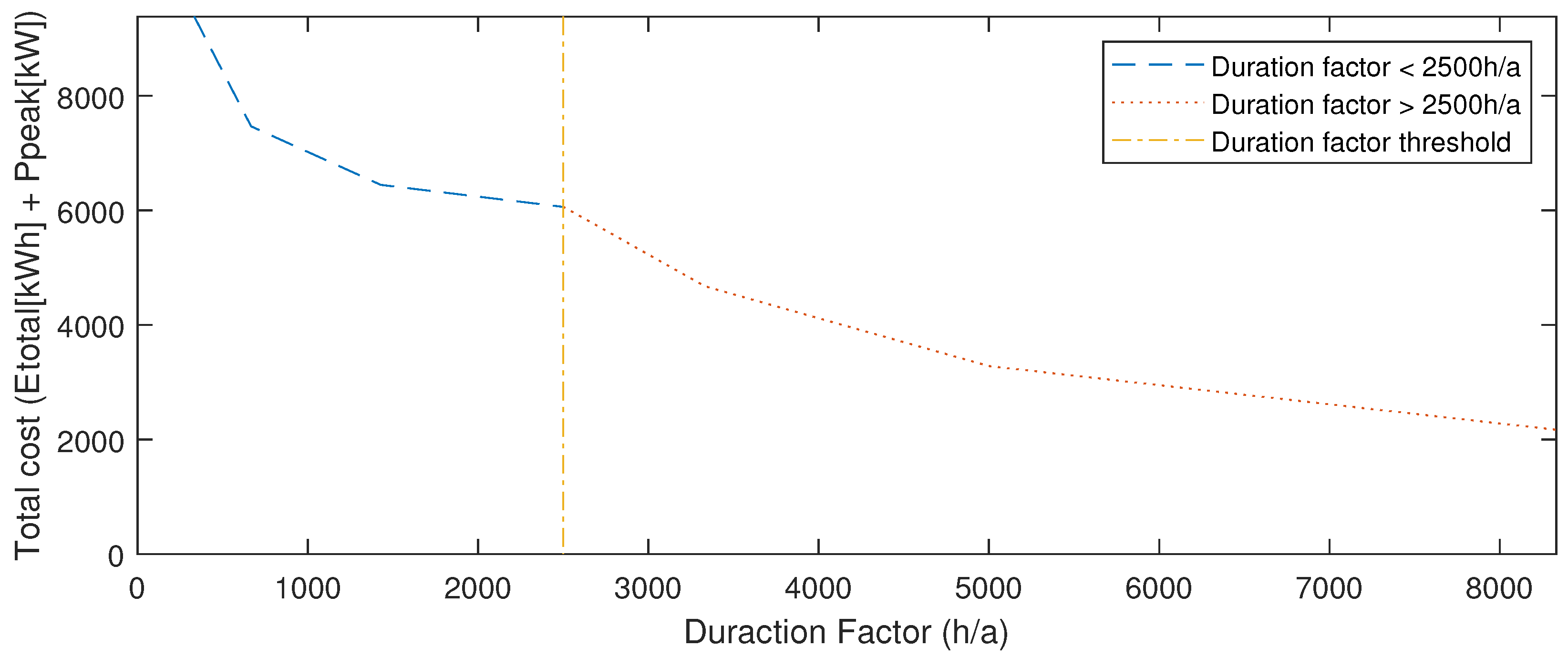
The economically optimal battery storage component sizing for an industrial customer equipped with storage system is obtained using LP. The load demand profiles considered in this study cover one full year, to capture all seasons with their characteristic. As the intent is to minimize the overall electricity cost, three types of costs are considered: the energy cost $C_{\mathrm{energy}\_\mathrm{tot}}$, the power cost $C_{\mathrm{power}\_\max }$, and the battery degradation cost $C_{\mathrm{storage}\_\mathrm{deg}}$. The energy cost is composed of the base energy price, fees, taxes, and stock exchange price. The power cost is charged by the network operator on the basis of the duration factor. The battery degradation cost, also called aging cost, is the major cost driver during storage operation, caused by cyclic and calendric aging.

The annual cost flow analysis presented here takes into account the discounted storage cost caused by degradation. As such, this simulation allows to estimate the profitability of a BESS for a full life of the battery.

All variables and parameters considered in this study are described in

Table 2. Variables and parameters used for the battery modeling and optimization routines.

Variable	Description (At the Time Slot i)	Unit	Constraints/Comments
$P_{{\mathrm{load}}_i}$	load demand (historical data)	kW	≥0; input data
$P_{\mathrm{inv}}^{\mathrm{nom}}$	Nominal power of the battery inverter	kW	Subject to optimization
${\mathrm{E}}_{\mathrm{batt}}^{\mathrm{nom}}$	Nominal battery capacity	kWh	Subject to optimization
$P_{\mathrm{peak}-\mathrm{shave}}$	Maximum power for the full year	kW	Subject to optimization
$P_{\mathrm{batt}}$	Bidirectional power flow to the battery	kW	Result of optimization
$P_{{\mathrm{batt}-\mathrm{load}}_i}$	Power transferred from the battery to the load	kW	See Equation (8)
$P_{{\mathrm{grid}-\mathrm{load}}_i}$	Power imported from the grid to the load	kW	≥0; see Equations (8) and (9)
$P_{{\mathrm{grid}-\mathrm{batt}}_i}$	Power imported from the grid to the battery	kW	≥0; see Equation (9)
${\mathrm{SoH}}_i$	State of health	p.u.	$[0\dots 1]$; see Equation (14)
${\mathrm{E}}_{{\mathrm{batt}}_i}$	Battery energy content at time i	kWh	See Equations (12) and (13)
${\mathrm{SoC}}_i$	State of charge	p.u.	$[{\mathrm{SoC}}_{\min }\dots {\mathrm{SoC}}_{\max }]$

.

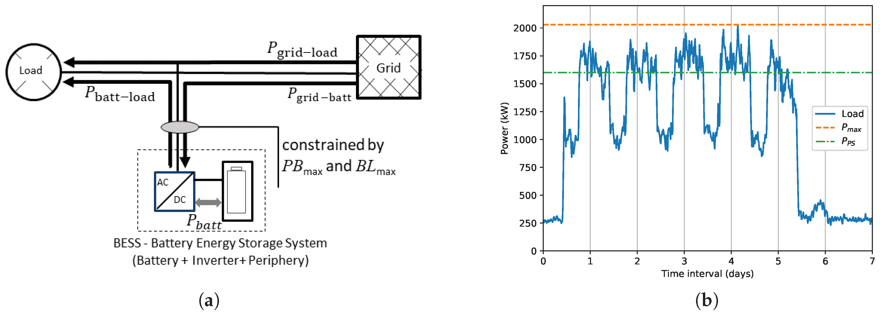
To meet the electrical demand, $P_{{\mathrm{load}}_i}$, the system attempts to use power from the battery, $P_{{\mathrm{batt}-\mathrm{load}}_i}$, or it draws power from the grid, $P_{{\mathrm{grid}-\mathrm{load}}_i}$, i.e.,

$$P_{{\mathrm{load}}_i}=P_{\mathrm{batt}-{\mathrm{load}}_i}+P_{\mathrm{grid}-{\mathrm{load}}_i}.$$

(8)

In the same way, the power imported from the grid ($P_{\mathrm{grid}-{\mathrm{load}}_i}+P_{\mathrm{grid}-{\mathrm{batt}}_i}$) in each time step i is restricted to the maximum power for the period. The two constraints can be represented as

$$P_{\mathrm{grid}-{\mathrm{load}}_i}+P_{\mathrm{grid}-{\mathrm{batt}}_i}\le P_{\mathrm{peak}-{\mathrm{shave}}_j},$$

(9)

where $P_{\mathrm{peak}-{\mathrm{shave}}_j}$ represents the highest point of demand in the billing period j. For instance, considering only the highest load of the year, all data points i should be limited to the same maximum annual limit $P_{\mathrm{peak}-{\mathrm{shave}}_j}$. However, if we consider the seasonal billing period where there are two independent thresholds, each season is limited to its own limit. The peak power is used to calculate the optimal solution power cost.

The bidirectional power flow from the storage inverter to the battery is stored in an auxiliary variable, $P_{{\mathrm{batt}}_i}$, and correlated with the inverter efficiency, ${\eta }_{\mathrm{inv}}$, as follows

$$P_{{\mathrm{batt}}_i}=({\eta }_{\mathrm{inv}}·P_{\mathrm{grid}-{\mathrm{batt}}_i})+(-\frac{1}{{\eta }_{\mathrm{inv}}}·P_{\mathrm{batt}-{\mathrm{load}}_i}),$$

(10)

where ${\eta }_{\mathrm{inv}}$ is the average one-way efficiency of the inverter. The reciprocal efficiencies are the battery charge power $P_{\mathrm{grid}-{\mathrm{batt}}_{\mathrm{i}}}$ and the discharge power, $P_{\mathrm{batt}-{\mathrm{load}}_{\mathrm{i}}}$, both limited by the nominal power flow from the inverter to the battery

$$\begin{array}{cc}\hfill 0\le & P_{\mathrm{grid}-{\mathrm{batt}}_i}\le P_{\mathrm{inv}}^{\mathrm{nom}},\hfill \\ \hfill 0\le & P_{\mathrm{batt}-{\mathrm{load}}_i}\le P_{\mathrm{inv}}^{\mathrm{nom}},\hfill \end{array}$$

(11)

where $P_{\mathrm{inv}}^{\mathrm{nom}}$ corresponds to the inverter size. The battery energy content at time step i (${\mathrm{E}}_{{\mathrm{batt}}_i}$) satisfies the recurrence relation

$${\mathrm{E}}_{{\mathrm{batt}}_i}=({\mathrm{E}}_{{\mathrm{batt}}_{i-1}}·\frac{{\mathrm{SD}}_{\mathrm{batt}}}{d})+({\eta }_{\mathrm{batt}}·P_{{\mathrm{batt}}_i}·\Delta t_{\mathrm{res}}),$$

(12)

where ${\mathrm{SD}}_{\mathrm{batt}}$ represents the self-discharge factor of the battery and $d=96$ the conversion factor of time steps per day. The energy content of the storage system is furthermore confined by an upper boundary, that decreases upon usage and aging according to the $\mathrm{SoH}$. The $\mathrm{SoH}$ is defined as the irreversible capacity fade over time, related to the nominal battery capacity, and $E_{{\mathrm{batt}}_i}$ is a fraction of the total energy content of the battery installed:

$${\mathrm{E}}_{{\mathrm{batt}}_i}\le {\mathrm{E}}_{\mathrm{batt}}^{\mathrm{nom}}·{\mathrm{SoH}}_i.$$

(13)

The state of health of the storage system at time step i also satisfies the recurrence relation

$${\mathrm{SoH}}_i={\mathrm{SoH}}_{i-1}-0.2·({\mathrm{aging}}_{{\mathrm{cal}}_i}+{\mathrm{aging}}_{{\mathrm{cyc}}_i}).$$

(14)

Using Equations (6) and (7), the calendric and cyclic aging can be estimated as

$$\begin{array}{cc}\hfill {\mathrm{aging}}_{{\mathrm{cal}}_i}=& (3.676\times {10}^{-7}·\mathrm{SoC}+6.246\times {10}^{-6})·(i·\Delta t_{\mathrm{res}})\hfill \end{array}$$

(15)

and

$${\mathrm{aging}}_{{\mathrm{cyc}}_i}={\mathrm{aging}}_{{\mathrm{cyc}}_{i-1}}+0.5·\frac{\left|P_{{\mathrm{batt}}_i}·\Delta t_{\mathrm{res}}\right|}{E_{{\mathrm{batt}}_i}}·\frac{1}{{\mathrm{Life}}_{\mathrm{Cyc}}^{80\%}}·$$

(16)

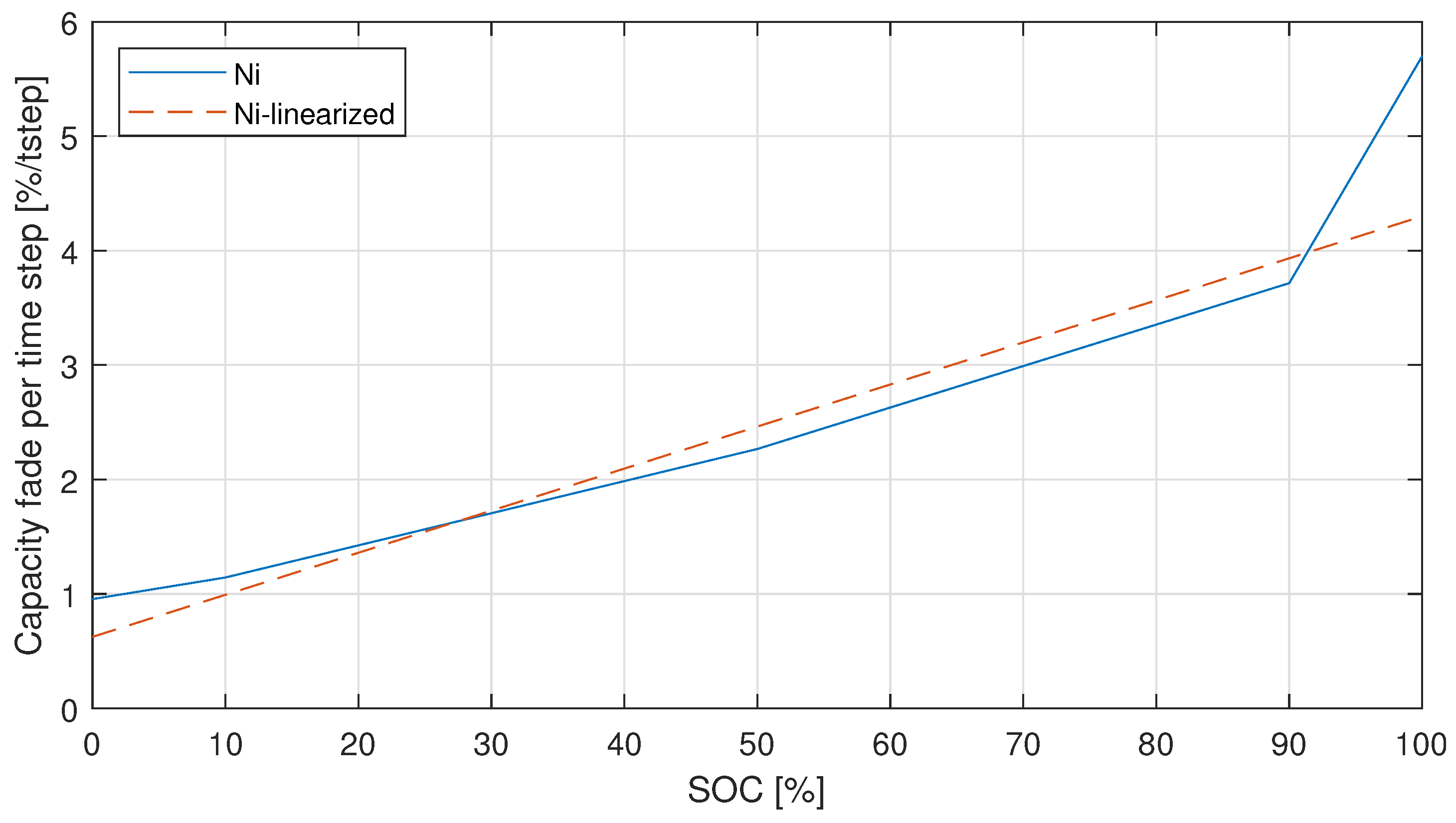
The calendric aging is affected by the storage temperature and its $\mathrm{SoC}$ level according to Swierczynski et al. [32]. Despite the fact that the charge/discharge process leads to dissipative heat generation and unavoidable temperature changes within the battery, the very low utilization ratio of the storage system and the restriction to a maximum C-rate of 3 limits the effects of temperature variations significantly.

As a result, the additional cyclic aging degradation of time step i is estimated by the energy throughput in time step i $(P_{{\mathrm{batt}}_j}·\Delta t_{\mathrm{res}})$ divided by the energy content of the system $E_{{\mathrm{batt}}_i}$ and is normalized with the factor of 0.5 and the technology specific cycle life indicator ${\mathrm{Life}}_{\mathrm{Cyc}}^{80\%}$. Similarly, the $\mathrm{SoC}$ can be expressed as

$${\mathrm{SoC}}_i=\frac{{\mathrm{E}}_{{\mathrm{batt}}_i}}{{\mathrm{E}}_{\mathrm{batt}}^{\mathrm{usable}}·{\mathrm{SoH}}_i}.$$

(17)

The inverter nominal power is limited to three times the battery nominal capacity

$${\mathrm{E}}_{\mathrm{batt}}^{\mathrm{nom}}\ge 3·P_{\mathrm{inv}}^{\mathrm{nom}}.$$

(18)

The optimal solution must satisfy all constraints described above. It aims to reduce the overall cost by minimizing the expenses for energy purchase and implicit cost caused by battery degradation. This cost model is divided into three components, i.e.,

$$\mathrm{minimize}{C}_{\mathrm{energy}\_\mathrm{tot}}+C_{\mathrm{power}\_\max }+C_{\mathrm{storage}\_\mathrm{deg}}.$$

(19)

The first component $C_{\mathrm{energy}\_\mathrm{tot}}$ comprises the cost of energy purchased from the grid, while the second component $C_{\mathrm{power}\_\max }$ is the peak induced cost based on the highest point of demand (or peak) within billing period (monthly or annually). These two components are evaluated as follows:

$$C_{\mathrm{energy}\_\mathrm{tot}}=\sum _i{C}_{\mathrm{buy}}·(P_{{\mathrm{grid}-\mathrm{load}}_i}+P_{{\mathrm{grid}-\mathrm{batt}}_i}),$$

(20)

$$C_{\mathrm{power}\_\max }=C_{\mathrm{power}}·P_{\mathrm{peak}-\mathrm{shave}},$$

(21)

where $C_{\mathrm{buy}}$ and $C_{\mathrm{power}}$ are the retail electricity price and the peak-power tariff, respectively. The third component estimates the storage system degradation cost that can be represented as

$$C_{\mathrm{storage}\_\mathrm{deg}}=\frac{\Delta \mathrm{SoH}}{(1-{\alpha }_{\mathrm{Replace}})}·{\mathrm{E}}_{\mathrm{batt}}^{\mathrm{nom}}+P_{\mathrm{inv}}^{\mathrm{nom}}·\frac{\Delta t}{T_{\mathrm{inv}}},$$

(22)

where $\Delta t$ denotes the time span covered with the simulation (here one year) and $\Delta \mathrm{SoH}$ the total battery aging. The full battery related cost is then calculated in consideration of the initial installation investment cost.

3.2. Case Description

Four industrial load profiles (A–D) shown in Figure 5 are used to verify the effectiveness of the proposed model. Data used for simulations was adapted from real measurements and averaged with a resolution of $\Delta t_{\mathrm{res}}$ = 15 min [39]. This time discretization results from the fact that, in the model region, the 15 minutes demand average is registered and its maximum value is used for tariff calculation over a period of one month or one year [40]. It is assumed that temperature is kept stable at approximately 25 ${}^{\circ }$C. Parameters and price information for the BESS/inverter system used in the simulations are listed in

Table 3. Battery Energy Storage System(BESS)/inverter performance parameters and price information [17].

Variable	Parameter	Unit	Value
${\eta }_{\mathrm{inv}}$	Average one way inverter efficiency	%	97.5
$T_{\mathrm{inv}}$	Assumed inverter lifetime in years	years	20
${\eta }_{\mathrm{batt}}$	Battery round-trip efficiency	%	95
${\mathrm{SD}}_{\mathrm{batt}}$	Self-discharge per day	%	0.02
$[{\mathrm{SoC}}_{\min }\dots {\mathrm{SoC}}_{\max }]$	Usable SoC	%	5–95
${\mathrm{Life}}_{\mathrm{cal}}^{80\%}$	Battery calendric life indicator	years	13
${\mathrm{Life}}_{\mathrm{cyc}}^{80\%}$	Cycle life indicator in FEC	FEC	4500
$C_{\mathrm{var},\mathrm{inv}}$	Variable inverter cost	€/kW	1306
$C_{\mathrm{var},\mathrm{batt}}$	Variable battery cost	€/KWh	577
$C_{\mathrm{fix}}$	Fixed cost for storage (housing, cooling, and periphery)	€	580

.

As described in Section 2, the electricity cost has two main components: the total energy consumption, and the power peak cost in the billing period. According to German law StromNEV §19I, every grid operator is obligated to offer a monthly billing scheme, i.e., instead of the highest load of the year, the highest load of the month is the basis for the price per kW. Hence, this study considers both yearly and monthly billing schemes. The results presented in the next section describe not only the optimal BESS/inverter component sizes, but also the optimal billing scheme.

3.3. Effect of Sizing Considering BESS Degradation Cost

The objective function and the constraints structured in this study have linear relationships. This means that the effect of changing a decision variable is proportional to its magnitude. For this reason, the economically optimal battery storage component sizing for peak shaving is obtained using LP. The linear optimization was implemented in MATLAB (MathWorks, Natick, MA, USA) code using a dual-simplex algorithm, which is based on a conventional simplex algorithm on the dual problem [41]. Each one-year simulation considered 15-min time resolution, co-optimized the storage and inverter size, and took on average 700 s on a workstation with Intel Core i5 processor at 3.5 Ghz and 16 GB of memory.

The optimal storage and inverter size for each profile (A–D), as well as a number relevant technical and economical indicators, are presented in

Table 4. Economical and technical comparison of system optimization results.

Profile	Profile A		Profile B		Profile C		Profile D
Scheme	Year	Month	Year	Month	Year	Month	Year	Month
Peak Loading Capping	5%	6%	30%	13%	8%	1%	0%	0%
Battery Size (kWh)	39	51	57	21	1109	18	0	0
Inverter size (kW)	117	152	171	63	3326	55	0	0
${\Delta }_{\mathrm{feh}}$ (h/a)	4431	4453	1195	957	1517	1407	2709	2709
Investment (€)	72,601	91,962	97,187	42,351	3,266,112	37,126	0	0
Operation Cost (€)	1156	1512	1663	674	39,577	583	0	0
Saving Grid charges (€)	15,880	16,735	992	6666	7613	6173	0	0
Total Savings (€)	14,725	15,223	−671	5992	−31,964	5591	0	0
Total return (IRR)	19%	14%	−169%	11%	−171%	12%	0%	0%
Amortization Time (years)	5	6	–	7	–	7	0	0
Full equivalent cycles (FEC)	5	51	1	32	11	25	0	0
Number of capped peaks	20	243	5	751	176	185	0	0
SoH at the end of year	98.78%	97.76%	98.88%	98.19%	98.66%	98.34%	0.00%	0.00%

.

The investment comprises the overall cost ${\mathrm{C}}_{\mathrm{storage}}$ described in Equation (3). The operation cost, ${\mathrm{C}}_{\mathrm{opex},\mathrm{batt}}$, reflects the German market and is calculated as 0.6% of the investment plus 6 €/kW.

Table 5. Operation cost (OPEX) composition.

Insurance	0.30%
System management	0.20%
Service contract	1 €/kW
Maintenance reserve	5 €/kW
Administrative costs	0.10%

shows the OPEX components considered in this paper.

The total return equal to the internal return rate (IRR) [42], is calculated without inflation or price changes based on the total savings of the first year. Likewise, total savings and amortization time are static calculations

$$\mathrm{TotalSavings}=\mathrm{SavingsGridCharges}-\mathrm{OPEX},$$

(23)

$$\mathrm{AmortizationTime}=\frac{\mathrm{Investment}}{\mathrm{TotalSavings}}·$$

(24)

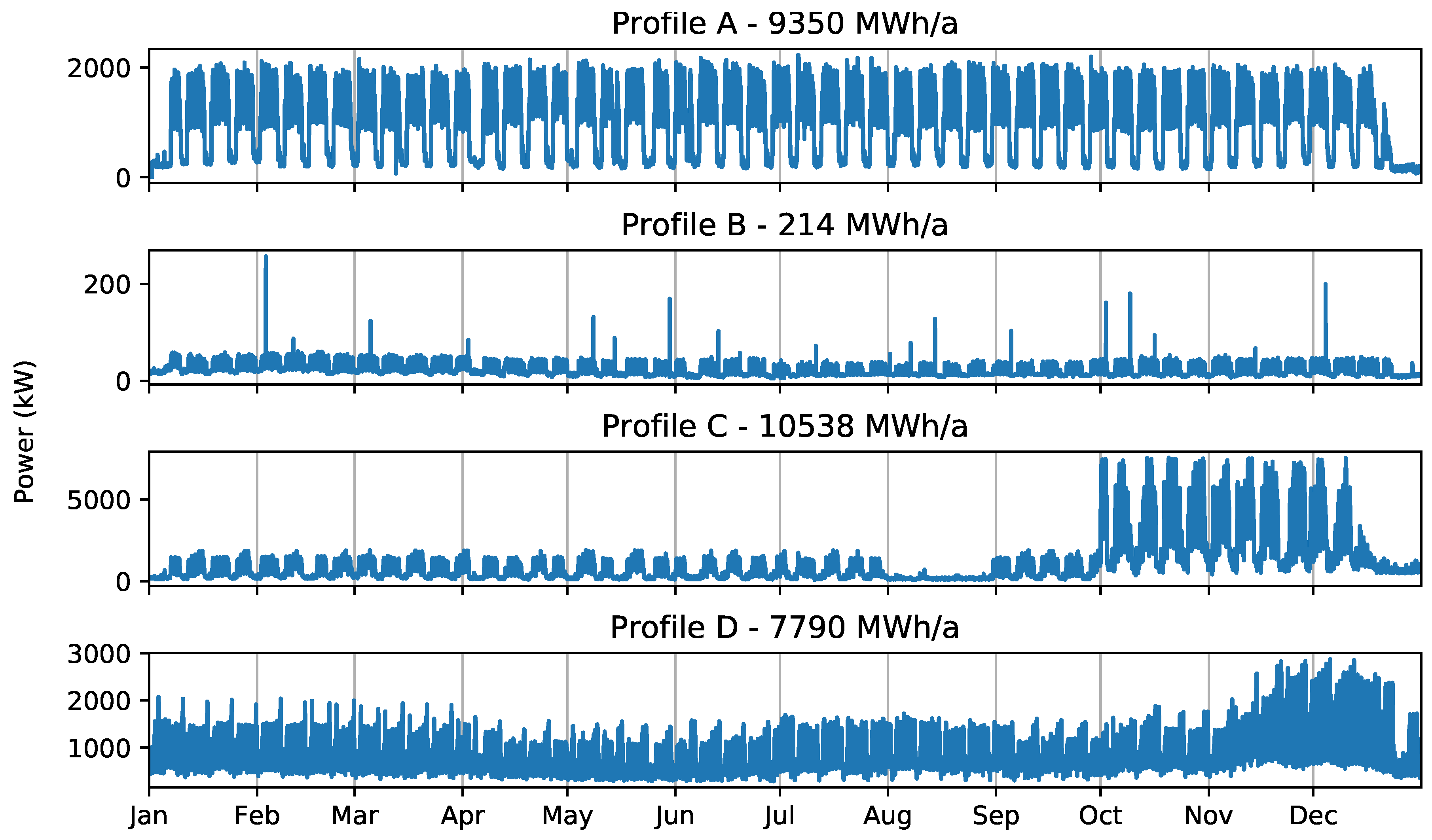
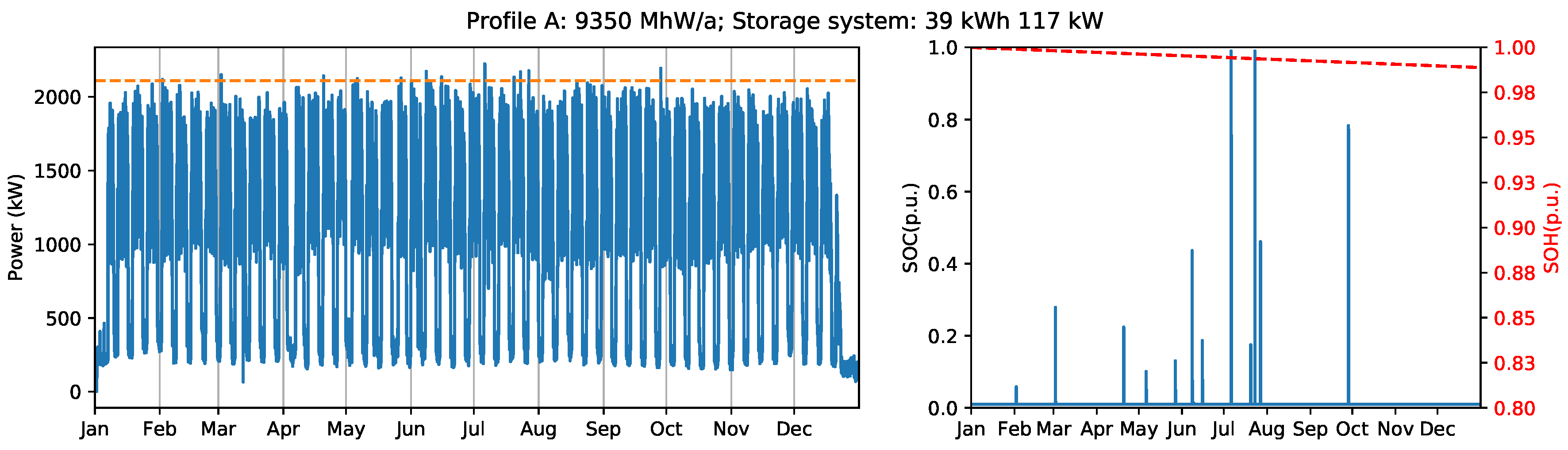
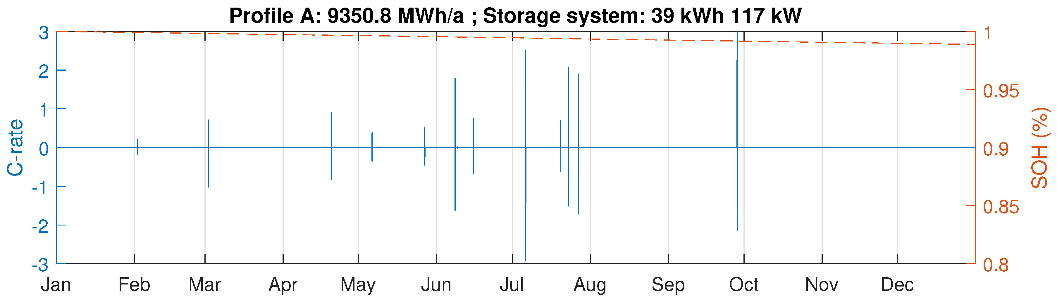
‘Profile A’ has an annual load of 9350 MWh and features weekday peaks and small load during weekends. As shown in Table 4, this profile exhibits similar results for yearly and monthly billing scheme. Figure 6 and Figure 7 illustrate the results obtained for the two billing schemes.

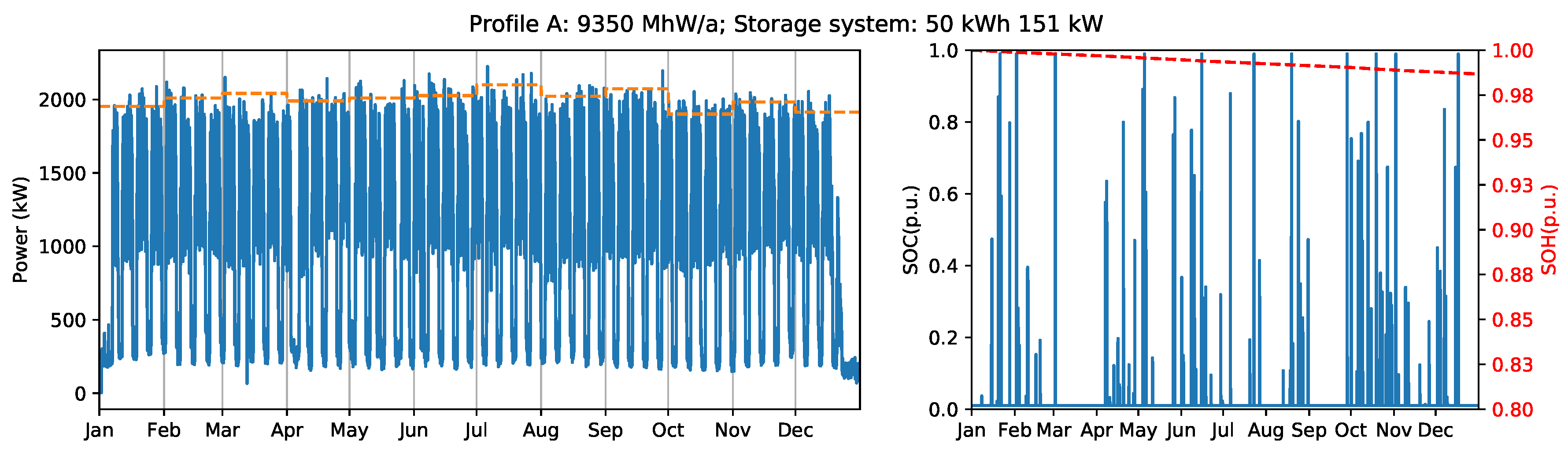
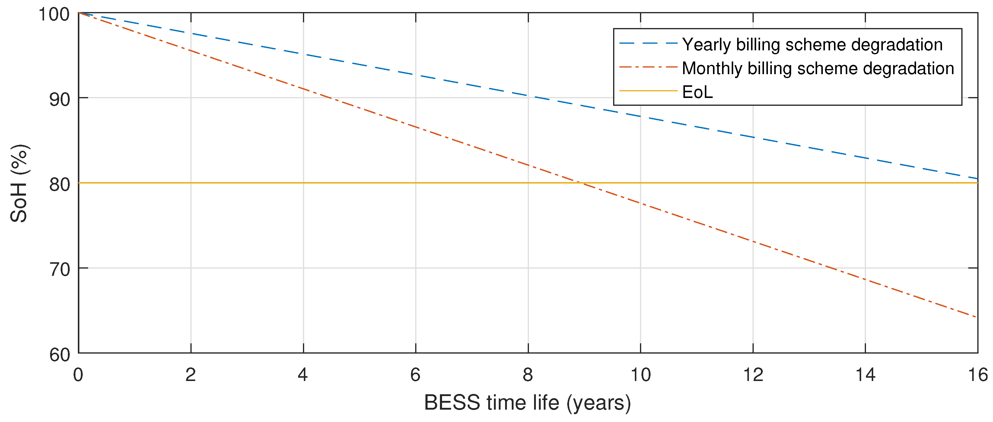
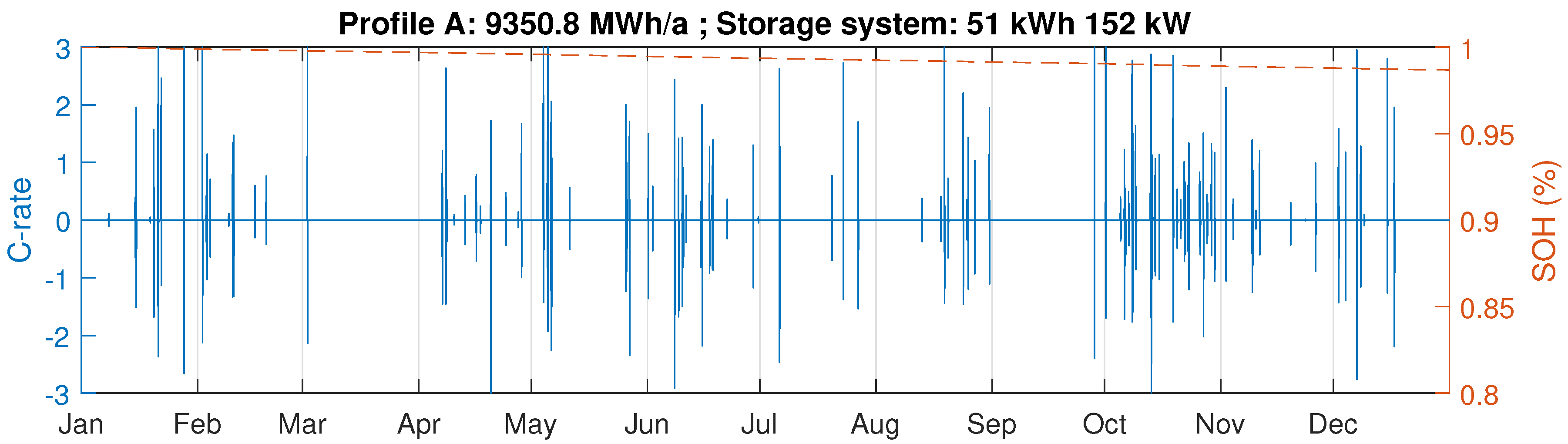
The yearly billing scheme requires an initial investment of almost €20.000 less compared to the cost of the system optimized for monthly billing, and it can generate additional 5% of total return in a shorter time. Although monthly billing scheme with a 51 kWh battery and 152 kW inverter (Figure 7) can increase the peak load capping, it also shortens the battery end of life by seven years (Figure 8). Therefore, all things considered, the yearly billing scheme is more suitable for ‘Profile A’ because it delays the battery replacement and provides several extra years of saving grid charges before it becomes necessary to invest in a new battery system.

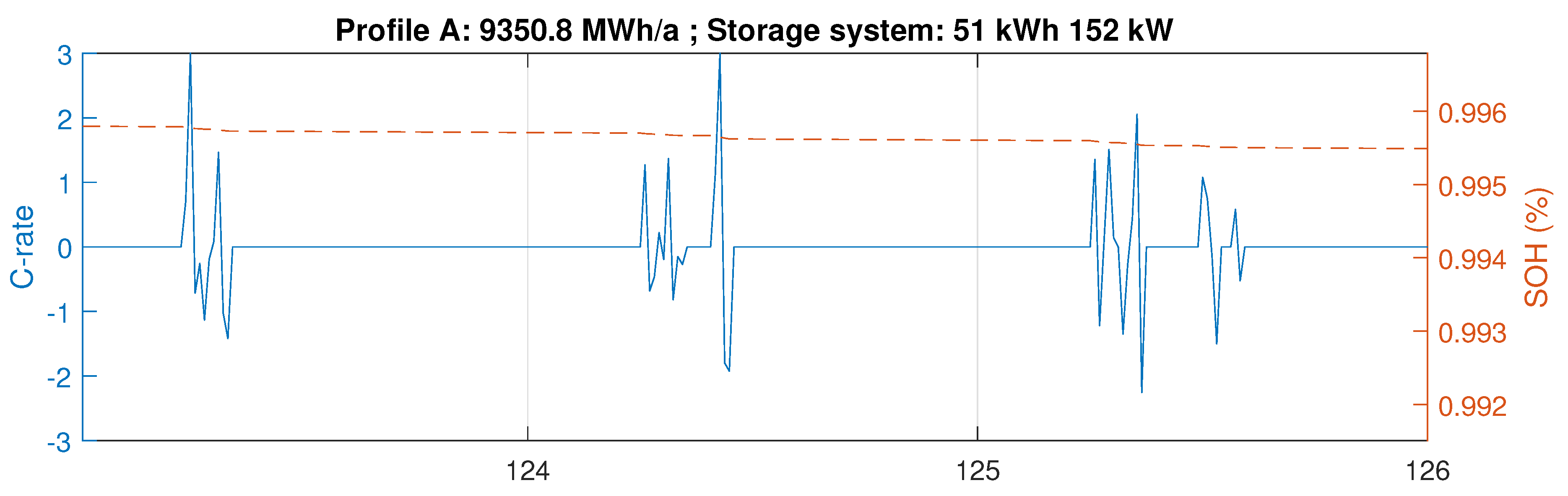
Further considering the monthly billing scheme, the optimizer determines the optimal storage size of 51 kWh and inverter nominal power of 152 kW. Figure 9 illustrates the power flows for a three-day period during the first week of May. The left panel shows the load consumption, the power flow imported from the grid for direct use or to charge the battery, as well as the maximum power peak after shave. The right panel shows the periodically changing charge level of the storage system ($\mathrm{SoC}$), and the evolution of battery degradation ($\mathrm{SoH}$). It clearly shows that the capacity fade is stronger when the energy throughput is high. Figure 10 shows the battery power profile and the same capacity fade in the terms of C-rate.

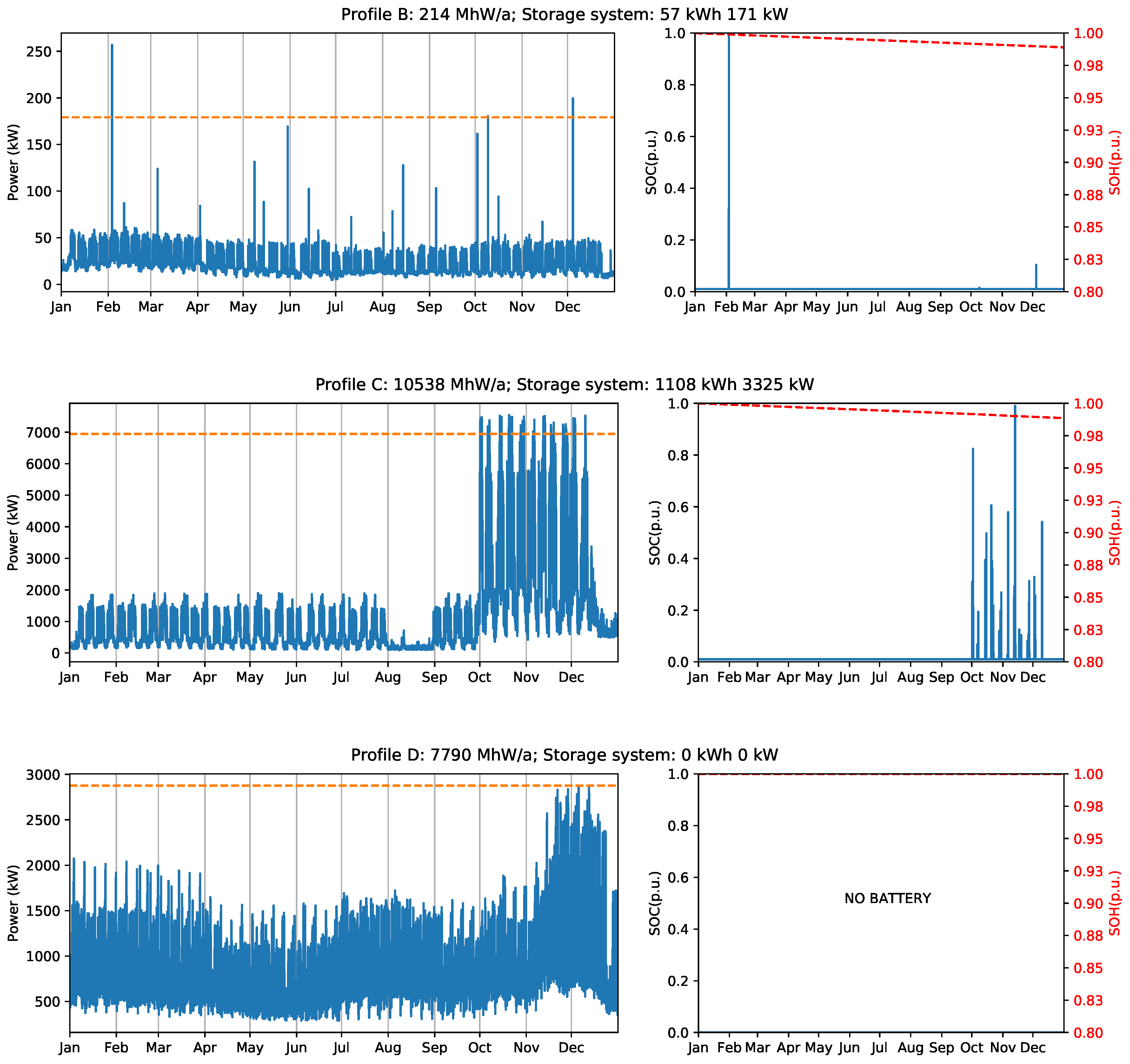
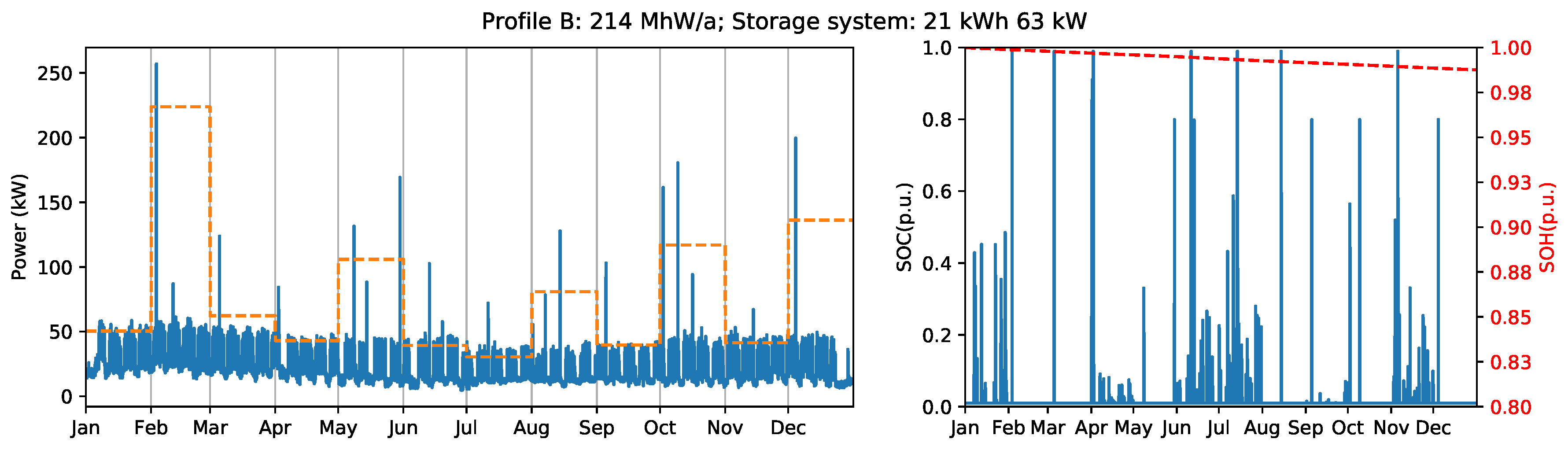
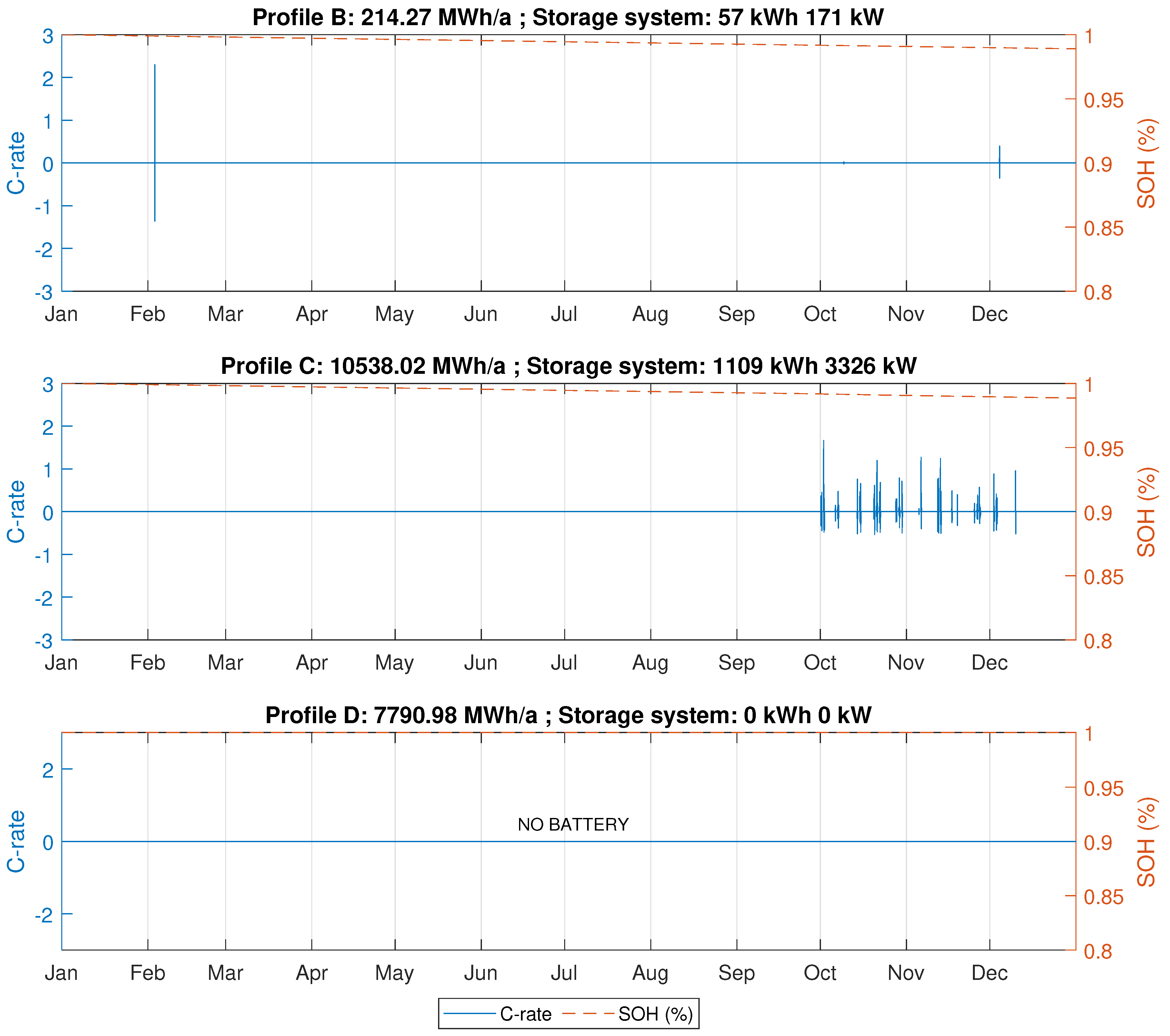
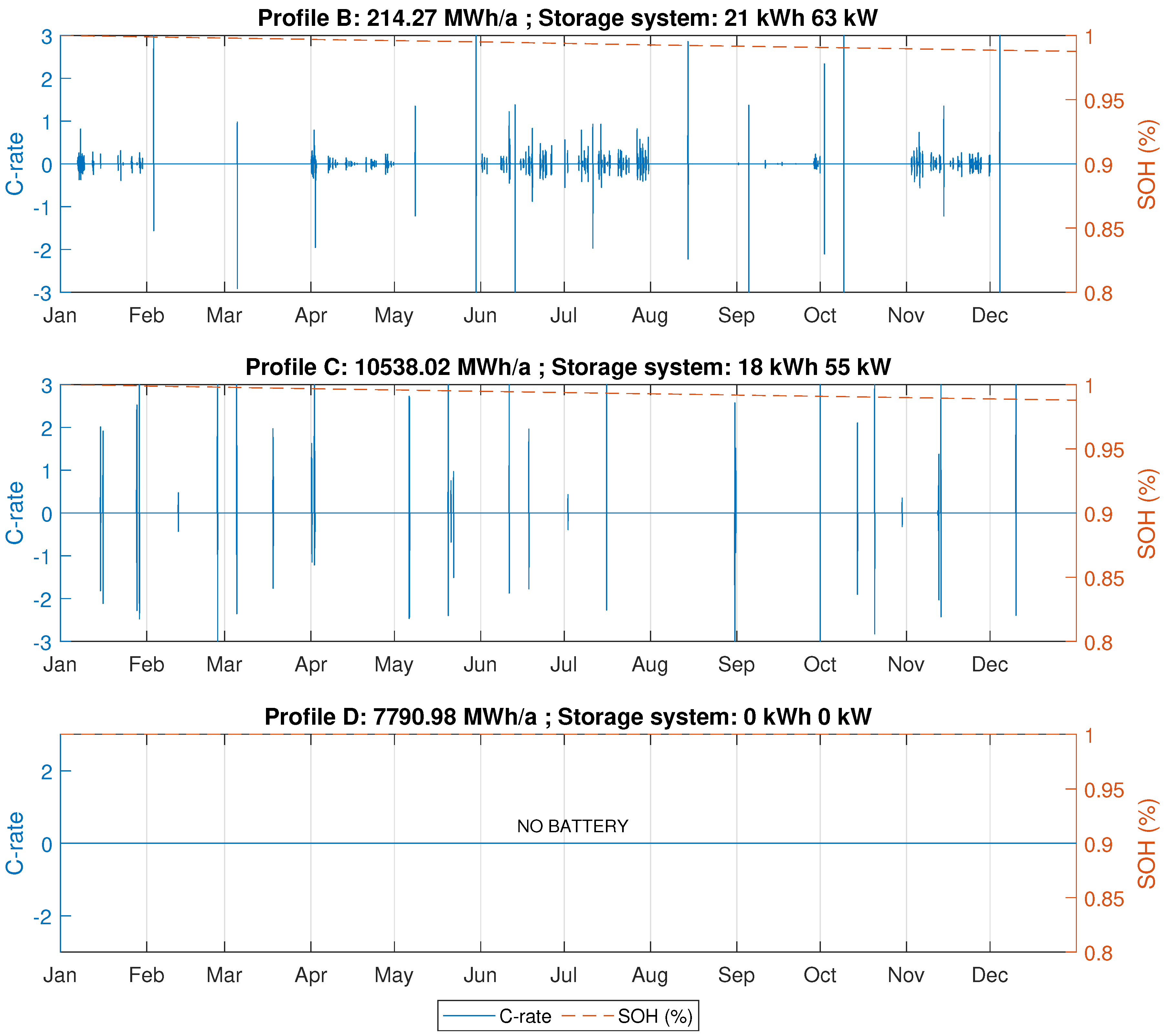
In contrast to ‘Profile A’, results for ‘Profile B’ show that the yearly billing scheme is not suitable for profiles with low average load and relatively high peaks. Although it is possible to reduce 30% of the peak load using a 57 kWh BESS with 171 kW inverter, this system configuration provides no savings to support the initial investment. In this case, the monthly scheme is more profitable, resulting in a peak reduction of 13% with a 21 kWh battery and 63 kW inverter.

Similarly, ‘Profile C’ has a negative IRR when considering the yearly billing scheme. This is caused by the seasonal nature of the load. As can be seen in Figure 5, the consumption in the last three months of the year is very high compared to the rest of the year. Analyzing the total return value in Table 4, the monthly billing scheme appears to be the right choice for this profile. However, a peak load reduction of only 1% is too slow to justify the installation of a BESS.

Finally, ’Profile D’ presents the most extreme case. Considering the exposed investment cost for BESS and price schemes, there is no advantage to installing a BESS for peak shaving purpose for this profile. Figure 11 illustrates the optimal annual peak shaving limit for the profiles B, C, and D, as well as the state of charge and state of health for the storage system used in each case. Similarly, Figure 12 shows the optimal monthly peak shaving limit, the $\mathrm{SoC}$, and $\mathrm{SoH}$ for the same three profiles. The Appendix A provides the battery power profiles for all investigated scenarios.

It can be seen that the optimization process minimizes expenses using the capacity of the storage system to decrease the peak power. The optimal power flow shows that the battery cycles are short, meaning that the battery is charged to the maximum necessary level just before being drained. This occurs due to the presence of $\mathrm{SoC}$-dependent calendric degradation as one of the optimization criteria. At the same, cyclic aging is not a determinant in peak shaving applications because the BESS has only a low number of charging/discharging cycles and energy is never stored in the battery for a long time. For this reason, calendric degradation is the most important cost driver in storage systems for peak shaving applications.

To analyze the relation between load size and return of investment, consider

Table 6. Profile A with yearly billing scheme and duration factor of 4431 h/a. Peak load capping of 5% which represents 20 capped peaks per annum.

Load (MWh/a)	Optimal		Recommended		Investment	Operation Cost	Saving Grid Charges	Total Savings (EBITDA)	Internal Rate of Return (IRR)	Payback (Years)	EoL (Years)	FEC (First Year)
	Battery Size	Inverter Size	Battery Size	Inverter Size
10	0	0	0	0	€0	€0	€0	€0	0%	0.00	0.00	0.00
25	0	0	0	0	€0	€0	€0	€0	0%	0.00	0.00	0.00
50	0	0	0	10	€0	€0	€0	€0	0%	0.00	0.00	0.00
100	0	0	0	10	€0	€0	€0	€0	0%	0.00	0.00	0.00
250	1	3	10	10	€18,370	€170	€425	€254	−15%	72.23	18.00	1.00
500	2	6	10	10	€18,370	€170	€849	€679	−7%	27.06	18.00	1.00
750	3	9	10	10	€18,370	€170	€1274	€1103	−1%	16.65	18.00	2.00
1000	4	13	10	20	€18,370	€230	€1698	€1468	2%	12.51	18.00	3.00
2500	10	31	20	40	€31,901	€431	€4246	€3814	8%	8.36	18.00	4.00
5000	21	63	30	70	€42,351	€674	€8491	€7817	17%	5.42	18.00	5.00
10,000	42	126	50	130	€86,737	€1300	€16,983	€15,682	16%	5.53	18.00	6.00
20,000	84	251	90	260	€175,619	€2614	€33,966	€31,352	16%	5.60	18.00	7.00
30,000	126	377	130	380	€222,974	€3618	€50,948	€47,331	20%	4.71	18.00	7.00
40,000	168	503	170	510	€286,941	€4782	€67,931	€63,150	21%	4.54	18.00	7.00

. Optimization runs were performed scaling the load size of Profile A from 10 to 40,000 MWh/a. The relation between the peaks and the loads were kept the same as in the original profile, resulting in exactly the same shape of battery $\mathrm{SoC}$ profile. As an overall trend, customers with large loads require BESS with large storage size and large nominal power of the inverter. Loads smaller than 1000 MWh/a have a negative IRR and an extensive payback period, rendering them unsuitable for BESS-based peak shaving applications. On the other hand, larger load profiles have a substantial improvement in the payback period. The results show that the BESS can be used for almost 18 years before reaching end of life at $80\%$ of $\mathrm{SoH}$. Although the peak capping is the same in all simulations, the battery usage differs for each load size because of the assumed discrete sizing of BESS and inverters in steps of 10 kWh and 10 kW respectively.

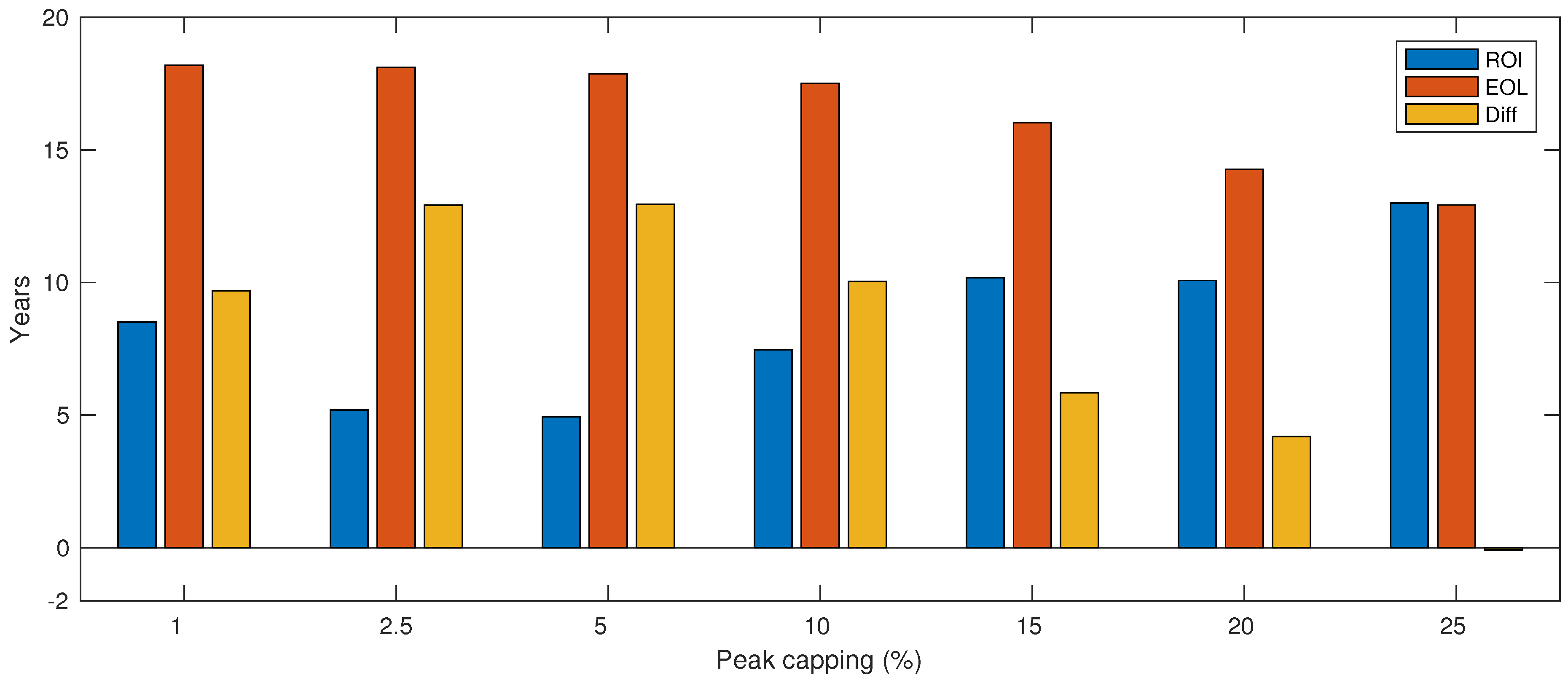
It is clear that larger load sizes can benefit from BESS-based peak shaving with better economical results. In addition, it is interesting to analyze the impact of the peak capping variation on the payback period as well as the battery life time. Refer to Figure 13 and

Table 7. Profile A wich peak load capping variating from 1% to 25%.

Peak Load Capping	Number of Capped Peaks	H/A	Load (MWh/a)	Recommended		Investment	Total Savings (EBITDA)	IRR	Payback (Years)	End of Life (Years)	Cycles
				Battery Size	Inverter Size
1%	1	4246	9351	10	30	€23,595	€2773	8%	8.51	18.19	1
3%	6	4311	9351	20	60	€37,126	€7154	18%	5.19	18.11	2
5%	20	4431	9351	40	120	€72,601	€14,721	19%	4.93	17.87	5
10%	217	4670	9351	250	230	€211,317	€28,300	10%	7.47	17.51	11
15%	1298	4945	9351	610	360	€424,782	€41,714	5%	10.18	16.02	34
20%	4185	5254	9351	1420	480	€560,915	€55,651	5%	10.08	14.27	69
25%	8008	5605	9351	2720	600	€945,282	€68,099	1%	13.88	12.92	101

for a detailed comparison. To generate these results, an additional constraint was added to the linear model described in Section 3.1

$$P_{\mathrm{peak}-\mathrm{shave}}=\max \left(P_{\mathrm{load}}\right)·(1-\mathrm{PC});\mathrm{PC}=[0.01,0.025,0.05,0.10,0.15,0.20,0.25,0.30],$$

(25)

where $\mathrm{PC}$ is the fixed amount of the peak that must be shaved. As shown in Table 7, all scenarios are profitable. However, the best IRR is obtained for peak capping equal to 5% of the total load. Smaller peak capping values extend the battery lifetime, but also extend the payback time as less savings of peak power reduction may be attained. In contrast, larger peak capping values increase the payback, but shorten the battery life.

As an overall trend, the increase of inverter size has a direct relation to the peak shaved load, i.e., 2.5% of load shaving needs a 60 kW inverter, and 25% load shaving requires ten times more. It is a straightforward relation because the inverter is sized according to the load power peak. Interestingly, the battery sizing does not follow the same trend because it is related to the number of peaks that must be shaved. In contrast to the optimal result where the battery is charged closer to the load peaks, larger peak load capping results in a smaller C-rate because the battery is charged slowly to avoid violating the maximum power peak allowed, and the battery must keep energy content for a longer period.

4. Conclusions and Future Work

This article describes a linear optimization model to size the most cost-effective BESS for a variety of industrial load profiles and multiple billing schemes. The optimization approach formulated in this work minimizes the storage degradation cost and the maximum power peak in the billing period.

The optimal BESS size and the number of capped peaks are directly related to the load profile. As an overall trend, for the exemplary load profiles under investigation, the monthly billing scheme is more attractive for industrial customers because of the number of peaks that can be capped with acceptable BESS sizes. For instance, a 51 kWh/152 kW BESS can shave 243 peaks which represents 6% of the maximum load peak and results in a 15,223 € of annual savings. As a general remark, considering the current cost of storage and retail energy tariff valid in Germany for 2016, most scenarios favor storage system installation. The expected increases of electricity prices and the reduction of BESS costs are likely to accelerate this trend. Although this work uses parameters corresponding to German market conditions and regulations, the described methodology can be easily adapted to other jurisdictions that use or consider peak power penalty, albeit with a different billing period scheme and retail electricity tariff models.

This work is limited to the optimization of storage systems using historical data on specific industrial load profile. Load forecast is the key to developing online energy management controllers for BESS. Such a forecasting task is outside the scope of this paper, but it will be considered in the future. Future work will also examine the possibility of decreasing the idle time of the battery system by sharing the same BESS between multiple industrial customers.