Short-Term Electricity Price Forecasting Model Using Interval-Valued Autoregressive Process

Abstract

The uncertainty that dominates in the functioning of the electricity market is of great significance and arises, generally, because of the time imbalance in electricity consumption rates and power plants’ production capacity, as well as the influence of many other factors (weather conditions, fuel costs, power plant operating costs, regulations, etc.). In this paper we try to incorporate this uncertainty in the electricity price forecasting model by applying interval numbers to express the price of electricity, with no intention of exploring influencing factors. This paper represents a hybrid model based on fuzzy C-mean clustering and the interval-valued autoregressive process for forecasting the short-term electricity price. A fuzzy C-mean algorithm was used to create interval time series to be forecasted by the interval autoregressive process. In this way, the efficiency of forecasting is improved because we predict the interval, not the crisp value where the price will be. This approach increases the flexibility of the forecasting model.

1. Introduction

Over the last few decades, many models for forecasting electricity prices have been developed using different mathematical methods. Generally, these models are based on simulation techniques; time series analysis; autoregressive processes such as autoregressive, autoregressive integrated, autoregressive moving average and seasonal autoregressive methods; artificial neural network; fuzzy logic; grey system theory; game theory; and combinations of two or more methods. Weron explained the complexity of available solutions, their strengths and weaknesses, and the opportunities and threats that the forecasting tools offer or that may be encountered in the process of electricity price forecasting [1]. A very useful tutorial review of probabilistic electricity price forecasting that presented much-needed guidelines for the rigorous use of methods, measures and tests, in line with the paradigm of ‘maximizing sharpness subject to reliability,’ was created by Nowotarski and Weron [2]. With the introduction of deregulation to the power industry, the price of electricity has been the key to all activities in the power market. Accurately and efficiently forecasting electricity prices becomes more and more important. Accordingly, Shahidehpour et al. mainly described short-term electricity price forecasting models based on simulations, neural networks, conditional probability distribution, and risk analysis [3]. Electricity markets suffer from a severe case of over-dimensionality due to the lack of economic storage of the commodity and the scarcity and hedging formulations can help users to form dynamic replicating portfolios. By using this approach they can reduce the complexity of possible future price combinations [4]. Forecasting is an integral part of revenue management. Designing dynamic prices requires forecasts of future demand, and scheduling consumption requires forecasts of future prices. Dutta and Mitra described research on prices in the electricity sector. They showed how different methods, such as the dynamic regression model, the transfer function model, the autoregressive integrated moving average model, the artificial neural network technique, the kernel-based method, principal component analysis, exponential smoothing, ɛ-insensitive loss function support vector regression, trigonometric gray prediction, and the semi-parametric additive model, can be used for forecasting the price [5]. The main methodologies used in electricity price forecasting have been reviewed by Aggarwal et al. The following price-forecasting techniques have been covered: stochastic time series, causal models, and artificial intelligence-based models [6].

In a data-sparse electricity market, Cheng et al. applied a novel interval grey prediction model to forecast the mid-term electricity market clearing price [7]. Day-ahead price forecasting of a daily electricity market using autoregressive integrated moving average models was used by Contreras et al. to forecast today the 24 market clearing prices of tomorrow [8]. A modified version of geometric Brownian motion has been proposed by Barlow (2002) as a jump diffusion model for the stochastic modeling of spot power prices [9]. Fu and Li applied simulation of power system equipment to forecast the electricity price within the context of a competitive electricity market [10]. A hybrid electricity price forecasting model for the Finnish electricity spot market proposed by Voronin and Partanena was based on the autoregressive moving average process and a neural network [11]. A wavelet transformation-based neural network model has been applied by Aggarwal et al. to forecast price profile in a deregulated electricity market [12]. Ghodsi and Zakerinia made a hybrid of the autoregressive integrated moving average process, an artificial neural network, and fuzzy regression to forecast short-term electricity prices [13]. Yamin et al. used an artificial neural network and developed an adaptive short-term electricity price forecasting model [14]. Statistical techniques for the pre-processing of data and a multi-layer neural network for forecasting electricity price and price spike detection were used by Cerjan et al. to develop a hybrid model for short-term electricity price forecasting [15]. A method using modular feed-forward neural networks and fuzzy inference system for forecasting short-term electricity price was developed by Esfahani [16]. Autoregressive integrated moving average models, complemented by the use of generalized autoregressive conditional heteroscedasticity models and their variants to account for volatility, were used for univariate forecasting of Singapore’s weekly wholesale electricity prices [17]. Ziel and Weron conducted an extensive empirical study of short-term electricity price forecasting to address the long-standing question of whether the optimal model structure for electricity price forecasting is univariate or multivariate. They provided evidence that, despite having the edge in terms of overall predictive performance, the multivariate modeling framework does not uniformly outperform the univariate one across all 12 considered datasets, seasons of the year, or hours of the day, and at times is outperformed by the latter [18]. Gonzalez et al. proposed a new functional forecasting method that attempts to generalize the standard seasonal ARMAX time series model to the L² Hilbert space. The structure of the proposed model is a linear regression where functional parameters operate on functional variables [19]. A new approach to forecast day-ahead electricity market prices, whose methodology is divided into two parts (forecasting of the electricity price through autoregressive integrated moving average models and construction of a portfolio of autoregressive integrated moving average models per hour using stochastic programming) was created by Nieta et al. [20]. Neupane et al. employed an ensemble prediction model in which a group of different algorithms participates in forecasting one hour ahead the price for each hour of a day. They proposed two different strategies, namely, the fixed weight method and the varying weight method, for selecting each hour’s expert algorithm from the set of participating algorithms [21].

Alvarez et al. applied a partitioning–clustering technique to the electricity price time series to discover the behavior patterns of a series [22]. A combination of a fuzzy C-mean clustering algorithm and a teaching–learning-based optimization algorithm was used to forecast the next day’s electricity price [23]. Sokhanvar et al. proposed a method that involves input–output decomposition and a simple clustering algorithm to classify the data points. The prediction is then generated by using the weighted mean of forecasted outputs of some clusters with the highest probabilities [24]. A hybrid model of fuzzy C-elliptotypes of fuzzy clustering and an advanced general radial basis function network was developed to forecast electricity prices in the market [25].

This paper represents a hybrid model based on the fuzzy C-mean clustering and interval-valued autoregressive process for forecasting the short-term electricity price. A fuzzy C-mean algorithm is used to separate a set of monitored data into an adequate number of fuzzy states. Accordingly, we can create chronological fuzzy time series by inspection of what fuzzy state the monitored value belongs to. In many cases, creating fuzzy relations among fuzzy time series is very difficult. To avoid it, we represent a fuzzy time series by an interval time series. Every interval corresponds to an adequate fuzzy state, but is expressed by closed bounded set of real numbers. The lower bound of an interval is equal to the electricity price with a minimum value in the fuzzy state while the upper bound is the price with the maximum value. Generally, a fuzzy C-mean clustering algorithm can be treated as a data preprocessing phase, i.e., the preparation of data to be forecasted by the interval-valued autoregressive process. The main target of the data preprocessing is to decrease the volatility of the monitored states, because sometimes it is very hard to describe it adequately. Calibration of the forecasting model considers two main parameters. The first parameter represents the number of fuzzy states for a monitored electricity price series, while the second gives the order of the autoregressive process. To define the number of fuzzy states we developed an approach based on the autocorrelation function of the interval series created with respect to a given number of fuzzy states. The order of the autoregressive process is defined by Akaike and the Schwartz–Bayesian information criterion. The model was tested on the real monitored electricity price series and the accuracy of the model is very high.

2. Short-Term Forecasting Model

This paper investigates time invariant fuzzy time series of daily electricity prices. The investigation includes two main components. The first component refers to the fuzzification of monitored data using the fuzzy C-mean clustering algorithm, while the second refers to the creation of a forecasting model based on the interval-valued autoregressive process.

2.1. Fuzzification of Monitored Data

The fuzzy time series was originally defined by Song and Chissom [26,27]. The basic definitions of the fuzzy time series, and time-variant and time-invariant fuzzy time series, are given as follows.

Suppose that $X(t)\in R^1, t=0,1,2,\dots$ is the universe of monitored data that should be fuzzified by fuzzy sets $f_i(t), i=1,2,\dots$ and let $F(t)$ be a set of $f_i(t)$. Then, $F(t)$ is called a fuzzy time series on $X(t)$. If $F(t)$ is caused by $F(t-1)$, this dependency is defined as $F(t)=F(t-1)\ast R(t,t-1)$, where $R(t,t-1)$ is a fuzzy relation of the first order between $F(t)$ and $F(t-1)$ and * is the fuzzy operator. If $F(t)$ is caused by $F(t-1)$ and $R(t,t-1)$ is constant for each t, then $F(t)$ is a time-invariant fuzzy series.

The intention of fuzzification is to transform a series of monitored data into a series of fuzzy states. Using this approach, each value within a series is transferred into an adequate fuzzy state and we obtain the order of states instead of the order of discrete values. For that purpose, we apply the fuzzy C-mean clustering algorithm [28,29,30,31] over the set of daily monitored electricity prices, $P(i)=\{p_i\}, i=1,2,\dots ,N$.

A fuzzy C-mean algorithm is a method based on the minimization of a generalized least-squared error function within groups. Let $P=\{p_i\}⫅R^{N\times 1}$ be the univariate series of monitored data and $C_m=\{c_m\}, m=1,2,\dots ,M$ be the electricity price vector composed of M cluster centers. Every cluster is a fuzzy set defined by the relative closeness to space $P=\{p_i\}⫅R^{N\times 1}$.

The membership degree $u_{im}\in [0,1]$ indicates to what degree the relative closeness P_N belongs to the cluster center vector C_m, which results in a fuzzy partition matrix $U={|u_{im}|}_{N\times M}$. Let u_im be the membership, C_m the center of the cluster, N the number of observed data points, and M the number of clusters. Then, the objective function, which should be minimized in fuzzy clustering, is defined as follows:

$$J=(U,c_1,c_2,\dots ,c_m,P)={\sum }_{i=1}^N{\sum }_{m=1}^M{u}_{im}^{\omega }{d}_{im}^2(p_i,c_m),$$

(1)

where d_mi is the Euclidean distance between the observation and the center of the cluster; $d_{im}=\sqrt{{(s_i-c_m)}^2}, i=1,2,\dots ,N$, and exponent ω is the fuzzy index ($\omega >1$). In this paper we set up $\omega =2$. The objective function J is minimized subject to the following constraints:

$${\sum }_{m=1}^M{u}_{im}=1,\hspace{1em}i=1,2,\dots ,N,$$

(2)

$$0\le u_{im}\le 1,\hspace{1em}m=1,2,\dots ,M,\hspace{1em}i=1,2,\dots ,N,$$

(3)

$$0<{\sum }_{i=1}^N{u}_{im}<m,\hspace{1em}m=1,2,\dots ,M.$$

(4)

An iterative algorithm is used to find the minimum of the objective function. In j-th iteration, the values of $u_{mi}^{\omega }$ and $c_m$ are updated as follows:

$$c_m=\frac{{\sum }_{i=1}^N{u}_{im}^{\omega }{p}_i}{{\sum }_{i=1}^N{u}_{im}^{\omega }},$$

(5)

$$u_{im}=\frac{{(\frac{1}{|p_i-c_m|})}^{\frac{1}{\omega -1}}}{{\sum }_{m=1}^M{(\frac{1}{|p_i-c_m|})}^{\frac{1}{\omega -1}}}.$$

(6)

The iteration process stops when $\left|\right|J^{(j+1)}-J^{(j)}\left|\right|<\delta$, where $\delta$ represents the minimum amount of improvement or a given threshold value.

The number of clusters represents the number of fuzzy sets or states. According to the obtained fuzzy partition matrix ($U={|u_{im}|}_{N\times M}$) we can define the fuzzy state matrix S(i) of the observed data as follows:

$$S(i)=\left[\begin{array}{c}\mathrm{s}(1)=max\{u_{11}(c_1),u_{12}(c_2),\dots ,u_{1M}(c_M)\}\\ \mathrm{s}(2)=max\{u_{21}(c_1),u_{22}(c_2),\dots ,u_{2M}(c_M)\}\\ ⋮\\ \mathrm{s}(N)=max\{u_{N1}(c_1),u_{N2}(c_2),\dots ,u_{NM}(c_M)\}\end{array}\right]$$

(7)

If we take into consideration that the fuzzy C-mean algorithm produces a sequence of M cluster centers, then, on the basis of the maximum value of the membership function we can determine the fuzzy state to which the i-th monitored value belongs. Finally, the sequence of fuzzy states $S(i)=\{\mathrm{s}(1),\mathrm{s}(2),\dots ,\mathrm{s}(N)\}$ represents a fuzzy time series on $P(i)=\{p_i\}, i=1,2,\dots ,N$.

The creation of fuzzy relations among obtained fuzzy states can be very complex. To overcome this problem, we transform the sequence of fuzzy states into an adequate stationary interval series and apply an interval-valued autoregressive process to create a short-term forecasting model.

2.2. Interval-Valued Forecasting Model

The process of transformation of a fuzzy time series into an interval time series is based on the fact that each fuzzy state $S_m(i), i\in \{1,2,\dots ,N\},m\in \{1,2,\dots ,M\}$ can be represented by a triplet; $S(i)=[c_m^{min}(i),c_m(i),c_m^{max}(i)]$, where $c_m^{min}(i)$ is equal to the element of the cluster with minimum value, $c_m^{max}(i)$ is equal to the element with the maximum value, and $c_m(i)$ is the center of the cluster. If we take into consideration that we monitored the daily electricity price then transformation produces the following interval time series:

$$P(i)\underset{C-mean}{\to }S(i);\left[\begin{array}{c}{p}_1\\ p_2\\ ⋮\\ p_i\\ ⋮\\ p_N\end{array}\right]\underset{C-mean}{\to }\left[\begin{array}{c}\left[p_1^l(m),p_1^u(m)\right]\\ \left[p_2^l(m),p_2^u(m)\right]\\ ⋮\\ \left[p_i^l(m),p_i^u(m)\right]\\ ⋮\\ \left[p_N^l(m),p_N^u(m)\right]\end{array}\right], m\in \{1,2,\dots ,M\},$$

(8)

where, $p_1^l(m)$ is the lowest and $p_1^u(m)$ is the highest daily electricity price for the m-th fuzzy state. Accordingly, we can say that we created chronological sequence of interval-valued data, i.e., we have a time series of interval data.

An interval variable X is defined as a closed, bounded set of real numbers in the form of $X=\left[x^l,x^u\right]$, where $x^l$ is the lower bound, $x^u$ is the upper bound of interval, and $x^l,x^u\in \Re$. An interval time series is a sequence of interval variables monitored in successive time points and expressed as a two-dimensional vector $X(i)={\left[x_i^l,x_i^u\right]}^T,i=1,2,\dots ,N$. In this paper we use the basic interval arithmetic operations introduced by Moore et al. [32]:

$$\begin{array}{l}X+Y=[x^l+y^l,x^u+y^u]\\ X-Y=[x^l-y^u,x^u-y^l]\\ X·Y=[min(x^l{y}^l,x^l{y}^u,x^u{y}^l,x^u{y}^u),max(x^l{y}^l,x^l{y}^u,x^u{y}^l,x^u{y}^u)]\\ \frac{X}{Y}=X·\frac{1}{Y}\\ \frac{1}{Y}=\left[\frac{1}{y^u},\frac{1}{y^l}\right],with 0\notin [y^l,y^u]\end{array}$$

(9)

The attraction of interval arithmetic is that it would not be necessary to analyze whether the conventional point-wise floating-point computations are safe. As the interval results contain all possible values, a narrow interval indicates success. A wide interval does not prove that a conventionally computed result is wrong, but it does indicate a risk. Interval arithmetic has the property of correctness; result intervals are guaranteed to contain the real number that is the value of the expression [33].

Every monitored series contains information about the process that generated it. This process can be realized by modeling the current value as a function of its previous values. An autoregressive process defines the current value of the variable as a weighted linear sum of its previous values and is defined as the following stochastic difference equation:

$$y_t={\beta }_0+{\sum }_{j=1}^k{\beta }_i{y}_{t-i}+{\epsilon }_t,$$

(10)

where, ${\beta }_0$ is a constant, ${\beta }_1,{\beta }_2,\dots ,{\beta }_k$ are coefficients of the model, ${\epsilon }_t$ is white noise (${\epsilon }_t~iidN(0,{\sigma }^2)$), and k is the order of the autoregressive process (lag). In the context of interval variables, the autoregressive process becomes an interval autoregressive process:

$$[y_t^l,y_t^u]=[{\beta }_0^l,{\beta }_0^u]+{\sum }_{j=1}^k[{\beta }_j^l,{\beta }_j^u][y_{t-j}^l,y_{t-j}^u]+[{\epsilon }_t^l,{\epsilon }_t^u].$$

(11)

Another representation of the interval can be done in terms of the so-called midpoint and radius, with $X^C=\frac{x^l+x^u}{2}$ and $X^R=\frac{x^u-x^l}{2}$. The midpoint is the center of an interval (the location), whereas the radius is the half-width of an interval (a measure of imprecision), with $X^R\ge 0$ [34]. Let $Y(i)=[y_i^C,y_i^R]$ be the interval response variable and $X(j)=[x_j^C,x_j^R]$ be the set of interval explanatory variables monitored on N units. Accordingly, Equation (11) can now be expressed by the following linear relationships:

$$y_i^C={\beta }_0^C+{\beta }_1^C{x}_{i-1}^C+{\beta }_2^C{x}_{i-2}^C+\dots +{\beta }_j^C{x}_{i-j}^C+{\epsilon }_i^C,$$

(12)

$$y_i^R={\beta }_0^R+{\beta }_1^R{x}_{i-1}^R+{\beta }_2^R{x}_{i-2}^R+\dots +{\beta }_j^R{x}_{i-j}^R+{\epsilon }_i^R,$$

(13)

where:

• $y_i^C$, $y_i^R$—the center and radius of the i-th interval response variable,
• $x_{i-j}^C$, $x_{i-j}^R$—the center and radius of the j-th interval explanatory variables,
• ${\beta }_0^C$, ${\beta }_0^R$—the center and radius of the constant,
• ${\beta }_j^C$, ${\beta }_j^R$—the center and radius of the regression coefficients of j-th interval explanatory variables,
• ${\epsilon }_i^C$, ${\epsilon }_i^R$—the center and radius of the residual of the i-th interval response variable.

The optimal coefficients are obtained according to the least-squares approach by minimizing the sum of squared residuals of $y_i^C$ and $y_i^R$ subject to non-negativity of ${\beta }_j^R$. The criterion of minimization is defined as:

$$\begin{array}{l}\underset{{\beta }_0^C,{\beta }_1^C,\dots ,{\beta }_j^C;{\beta }_0^R,{\beta }_1^R,\dots ,{\beta }_j^R}{\underbrace{min}}{\displaystyle {\displaystyle \sum }_{i=1}^k}[{({\epsilon }_i^C)}^2+{({\epsilon }_i^R)}^2]\\ {\beta }_j^R\ge 0,j=1,2,\dots ,k\end{array}$$

(14)

To define the values of the coefficients we apply the center and range method developed by Neto and de Carvalho [35]. The values of the coefficients ${\beta }_0^C,{\beta }_1^C,\dots ,{\beta }_j^C$ and ${\beta }_0^R,{\beta }_1^R,\dots ,{\beta }_j^R$ are the solutions of the following system of $2(k+1)$ normal equations written in matrix form:

$$\widehat{\beta }=({\widehat{\beta }}_0^C,{\widehat{\beta }}_1^C,\dots ,{\widehat{\beta }}_j^C,{\widehat{\beta }}_0^R,{\widehat{\beta }}_1^R,\dots ,{\widehat{\beta }}_j^R)={(A)}^{-1}\times b,$$

(15)

where A is a $2(k+1)\times 2(k+1)$ matrix and b is a $2(k+1)\times 1$ vector described as:

$$A=\left[\begin{array}{cccccccc}N& {\sum }_{i=1}^N{x}_{i-1}^C& \dots & {\sum }_{i=1}^N{x}_{i-k}^C& 0& 0& \dots & 0\\ {\sum }_{i=1}^N{x}_{i-1}^C& {\sum }_{i=1}^N{\left(x_{i-1}^C\right)}^2& \dots & {\sum }_{i=1}^N{x}_{i-k}^C{x}_{i-1}^C& 0& 0& \dots & 0\\ ⋮& ⋮& ⋮& ⋮& ⋮& ⋮& ⋮& ⋮\\ {\sum }_{i=1}^N{x}_{i-k}^C& {\sum }_{i=1}^N{x}_{i-1}^C{x}_{i-k}^C& \dots & {\sum }_{i=1}^N{\left(x_{i-k}^C\right)}^2& 0& 0& \dots & 0\\ 0& 0& \dots & 0& N& {\sum }_{i=1}^N{x}_{i-1}^R& \dots & {\sum }_{i=1}^N{x}_{i-k}^R\\ 0& 0& \dots & 0& {\sum }_{i=1}^N{x}_{i-1}^R& {\sum }_{i=1}^N{\left(x_{i-1}^R\right)}^2& \dots & {\sum }_{i=1}^N{x}_{i-k}^R{x}_{i-1}^R\\ ⋮& ⋮& ⋮& ⋮& ⋮& ⋮& ⋮& ⋮\\ 0& 0& \dots & 0& {\sum }_{i=1}^N{x}_{i-k}^R& {\sum }_{i=1}^N{x}_{i-1}^R{x}_{i-k}^R& \dots & {\sum }_{i=1}^N{\left(x_{i-k}^R\right)}^2\end{array}\right],$$

(16)

$$b={\left[{\sum }_{i=1}^N{y}_i^C,{\sum }_{i=1}^N{y}_i^C{x}_i^C,\dots ,{\sum }_{i=1}^N{y}_i^C{x}_{i-k}^C,{\sum }_{i=1}^N{y}_i^R,{\sum }_{i=1}^N{y}_i^R{x}_i^R,\dots ,{\sum }_{i=1}^N{y}_i^R{x}_{i-k}^R\right]}^T.$$

(17)

.

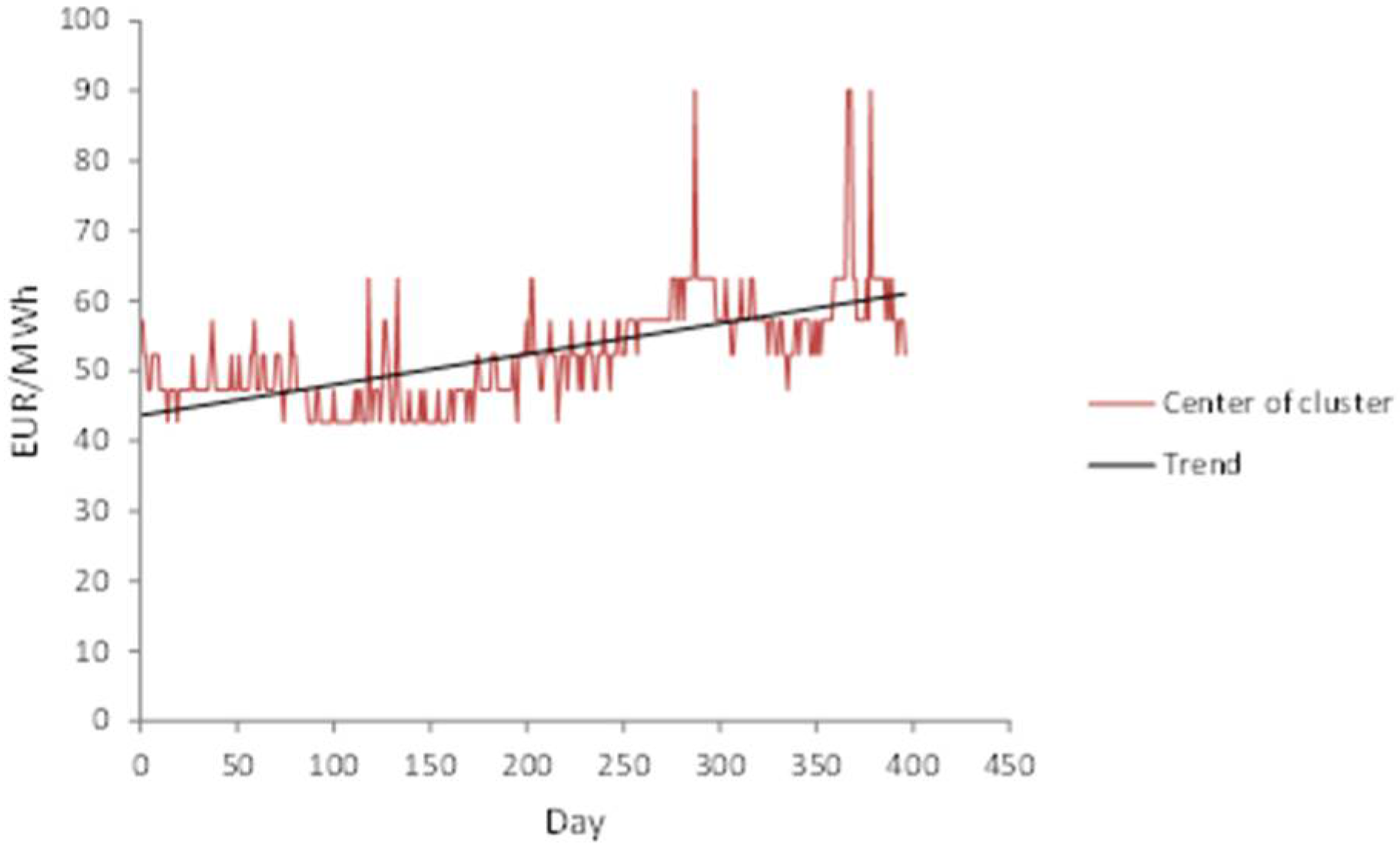
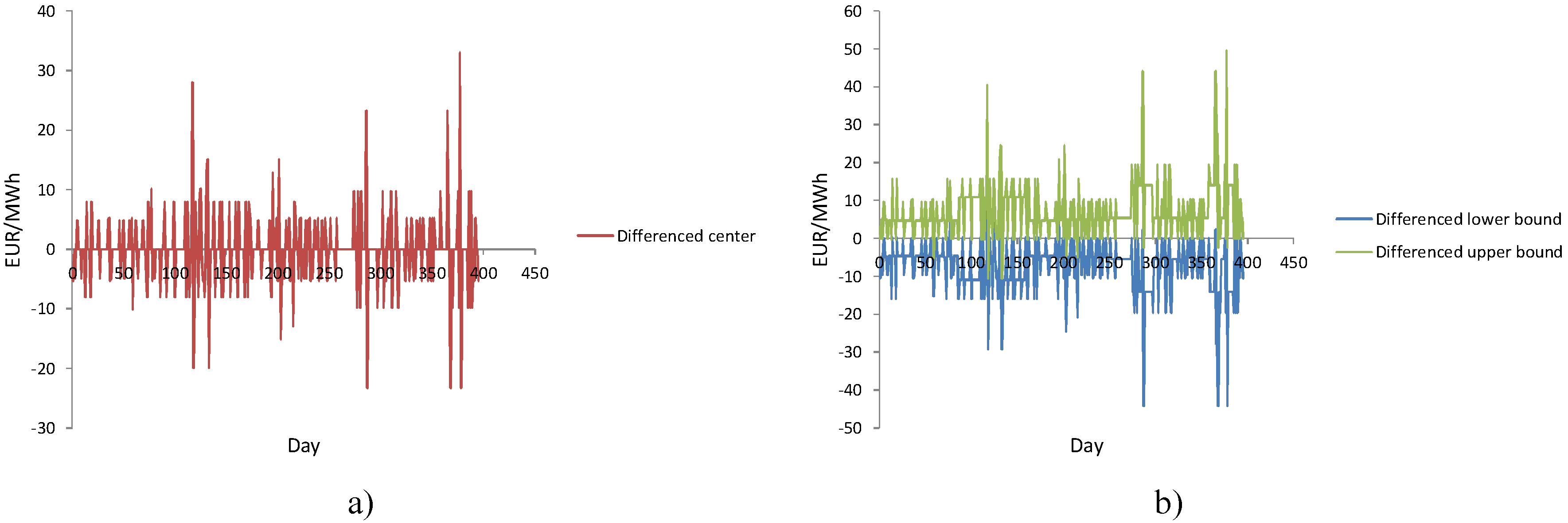
If the interval time series is stationary, then $d=0$; otherwise $d>0$, where d denotes the order of differencing. If the interval series is non-stationary, then it is necessary to transform it into a stationary series by d-differencing. First-order differencing is performed in the following manner:

$$\left[\Delta y_i^l,\Delta y_i^u\right]=\left[y_i^l,y_i^u\right]-\left[y_{i-1}^l,y_{i-1}^u\right], i=1,\dots ,N.$$

(18)

After differencing, the interval time series becomes stationary and we can apply the k-th interval autoregressive process (Equation (11)) on differenced series. Values of the interval differenced series will be forecasted as follows:

$$\left[\Delta {\widehat{y}}_i^l,\Delta {\widehat{y}}_i^u\right]=\left[\Delta {\widehat{y}}_i^C-{\widehat{y}}_i^R,\Delta {\widehat{y}}_i^C+{\widehat{y}}_i^R\right], i=1,\dots ,N.$$

(19)

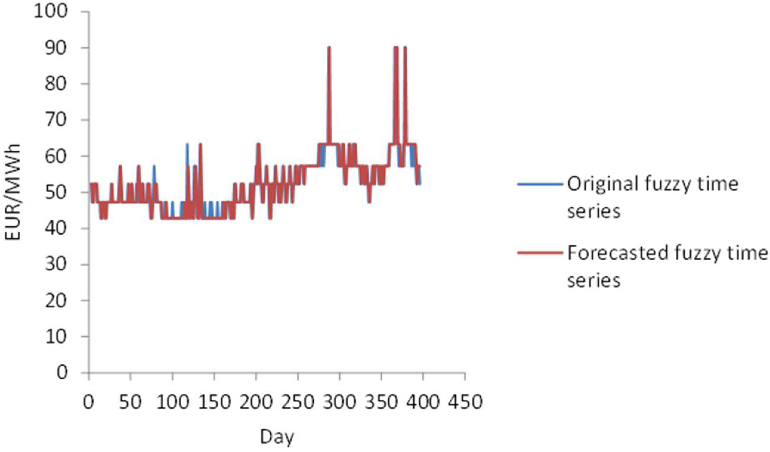
Equation (19) represents values for forecasting the first-order differenced series, but we want to forecast monitored electricity price series. Therefore, we must transform these values into the $\widehat{Y}(i)=\left[{\widehat{y}}_i^l,{\widehat{y}}_i^u\right],i=2,\dots ,N$ form as follows:

$$\left[\Delta {\widehat{y}}_i^l,\Delta {\widehat{y}}_i^u\right]=\left[\Delta {\widehat{y}}_i^C-{\widehat{y}}_i^R,\Delta {\widehat{y}}_i^C+{\widehat{y}}_i^R\right], i=1,\dots ,N.$$

(20)

If we take into consideration that the monitored series is represented by the series composed of M fuzzy states, then it is necessary to find out to which fuzzy state of M values the forecasted state corresponds. We propose the following procedure for expressing the sequence of forecasted fuzzy states by the set of M fuzzy states (Algorithm 1):

Algorithm 1:

Input: forecasted series by AR(k); $\widehat{P}(i), i=1,\dots ,N$

Output: forecasted fuzzy states expressed by M fuzzy states

Step 1. create series of forecasted centers; ${\widehat{p}}_i^C=\frac{{\widehat{p}}_i^l+{\widehat{p}}_i^u}{2}$

Step 2. create a fuzzy partition matrix; $\widehat{U}={\left|{\widehat{u}}_{im}\right|}_{N\times M}$

${\widehat{u}}_{im}=\frac{{\left(\frac{1}{\left|{\widehat{p}}_i^C-c_m\right|}\right)}^{\frac{1}{\omega -1}}}{{\sum }_{m=1}^M{\left(\frac{1}{\left|{\widehat{p}}_i^C-c_m\right|}\right)}^{\frac{1}{\omega -1}}}, m\in \{1,2,\dots ,M\}$

Step 3. create forecasted fuzzy state matrix; $\widehat{S}(i)$

$\widehat{S}(i)=\left[\begin{array}{l}\widehat{s}(1)=max\{{\widehat{u}}_{11}(c_1),{\widehat{u}}_{12}(c_2),\dots ,{\widehat{u}}_{1M}(c_M)\}\\ \widehat{s}(2)=max\{{\widehat{u}}_{21}(c_1),{\widehat{u}}_{22}(c_2),\dots ,{\widehat{u}}_{2M}(c_M)\}\\ ⋮\\ \widehat{s}(N)=max\{{\widehat{u}}_{N1}(c_1),{\widehat{u}}_{N2}(c_2),\dots ,{\widehat{u}}_{NM}(c_M)\}\end{array}\right]$

Step 4. create the sequence of forecasted fuzzy states; $\widehat{S}(i)=\{\mathrm{s}^(1), \mathrm{s} ^(2),\dots , \mathrm{s} ^(N)\}$

Step 5. according to $\widehat{S}(i)$ create interval forecasted series; $\widehat{P}(i,m)=[{\widehat{p}}_i^l(m),{\widehat{p}}_i^u(m)]$

Algorithm 1 represents the forecasting model. This algorithm is applied to forecast the future electricity price for $N+h, h=1,2,\dots ,H$. Note that this is a short-term forecasting model and H should be set to a few days.

Calibration of the forecasting model is related to the determination of two main parameters. The first parameter considers the number of fuzzy states (M-clusters) for a monitored electricity price series, while the second considers the order of the autoregressive process (k).

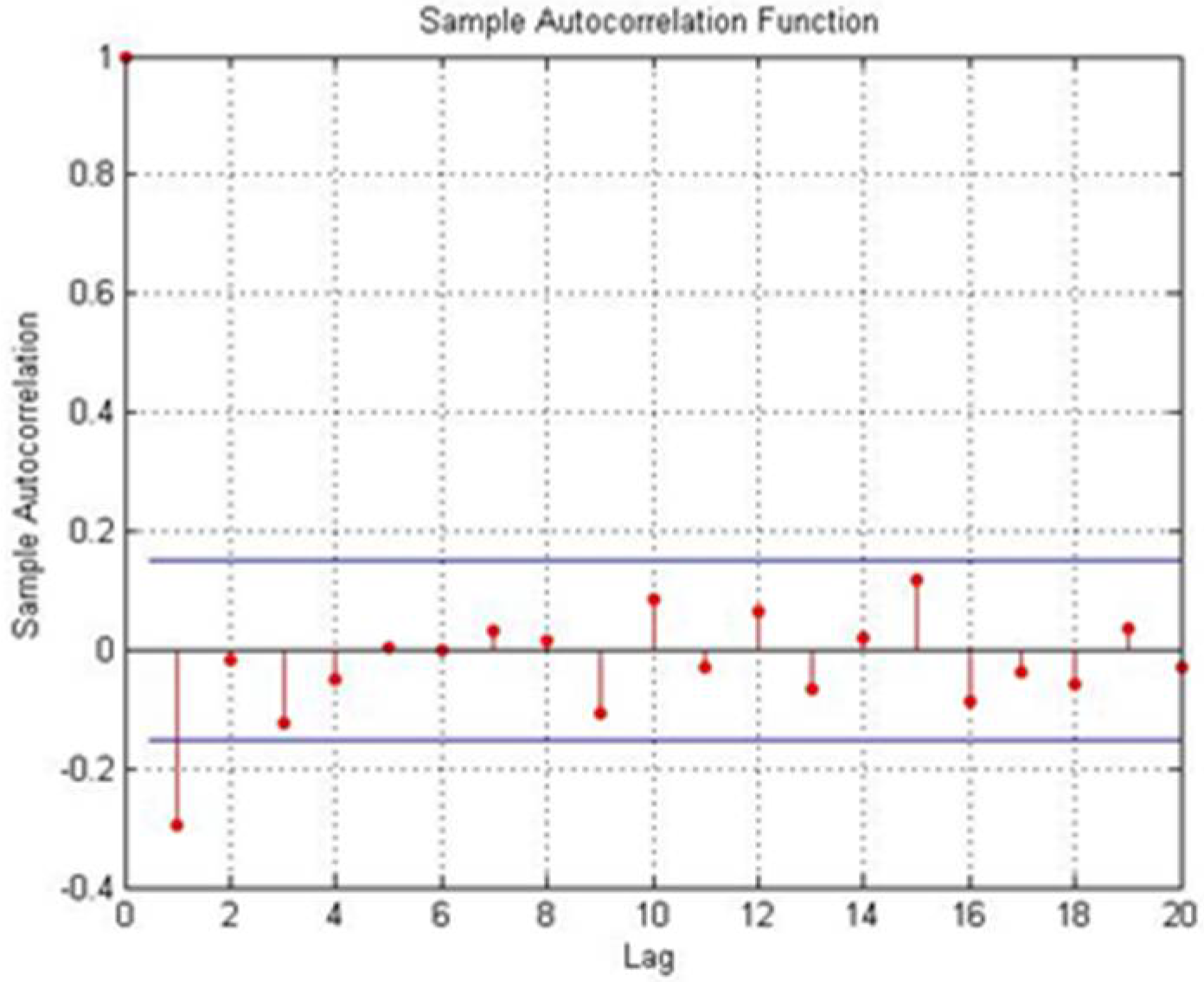
We developed the following iterative algorithm to define the minimum number of possible fuzzy states (clusters), (Algorithm 2):

Algorithm 2:

Input: monitored series $Y(i), i=1,2,\dots ,N$

Output: minimum number of clusters mmin

Step 1. set up the initial value of M to m = 3 and k = 20

Step 2. do the fuzzy C-mean

Step 3. create interval series $[y_i^l(m),y_i^u(m)], i=1,2,\dots ,N$

Step 4. if interval series is non-stationary do d-differencing

Step 5. create center series $y_i^C,i=1,\dots ,N$

Step 6. do autocorrelation function for 20 lags $ACF(y_i^C,20)$

Step 7. if there is one and only one lag such that $ACF(y_i^C,20)>\pm 2\times standard error$, stop.

Otherwise set m + 1 and go to Step 2

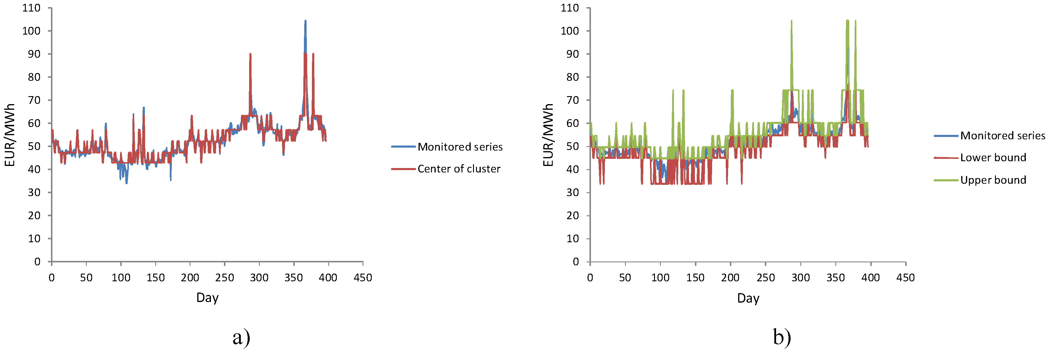
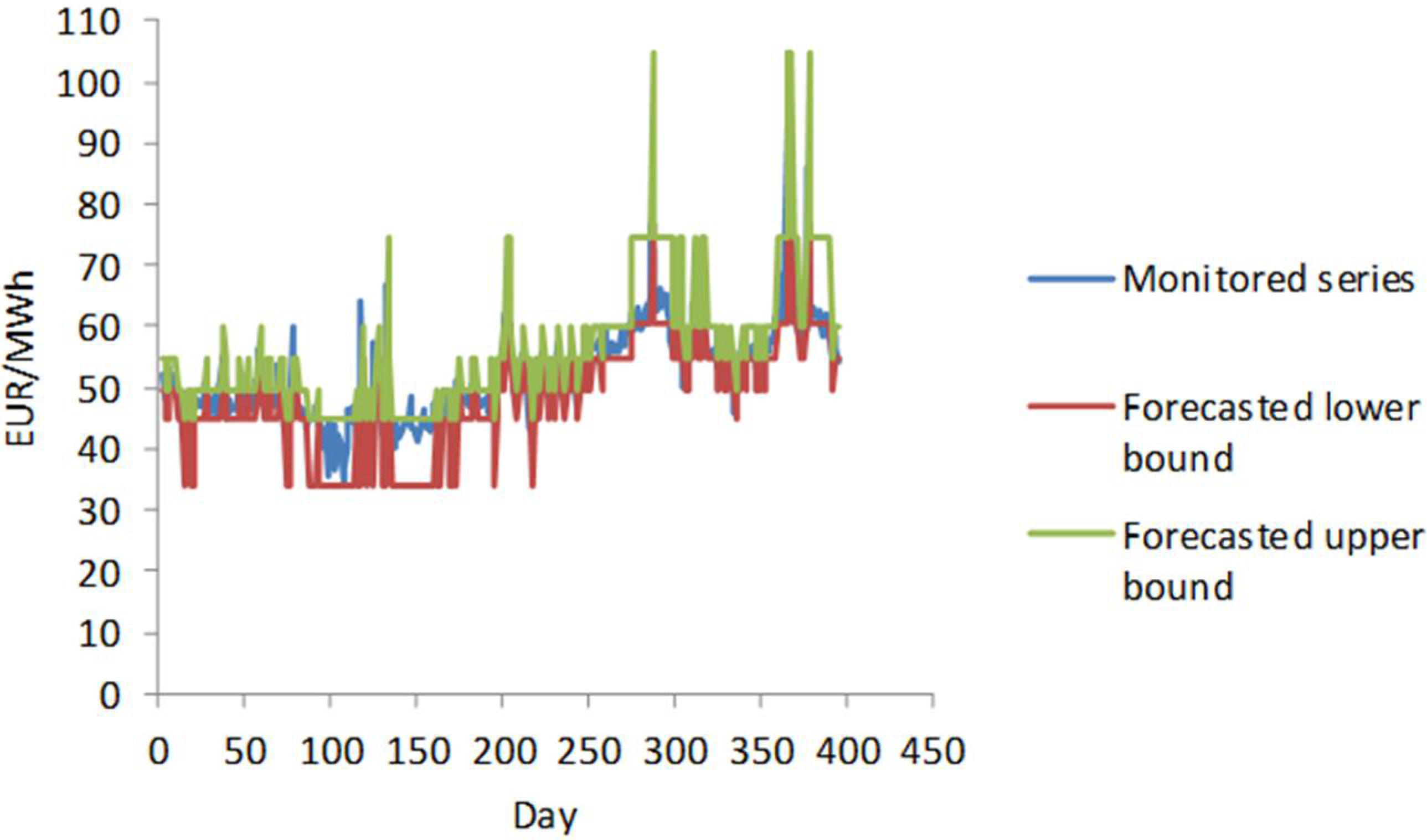
Figure 1 shows a case when the condition defined by Step 7 is met.

Figure 1. Autocorrelation function that satisfies the conditions.

The autocorrelation function (ACF) of any series gives the correlation between y_t and y_t−k for k = 1, 2, 3, …. Theoretically, the autocorrelation between y_t and y_t−k is calculated as:

$$ACF=\frac{Covariance(y_t,y_{t-k})}{Std.dev.(y_t)Std.dev.(y_{t-k})}.$$

(21)

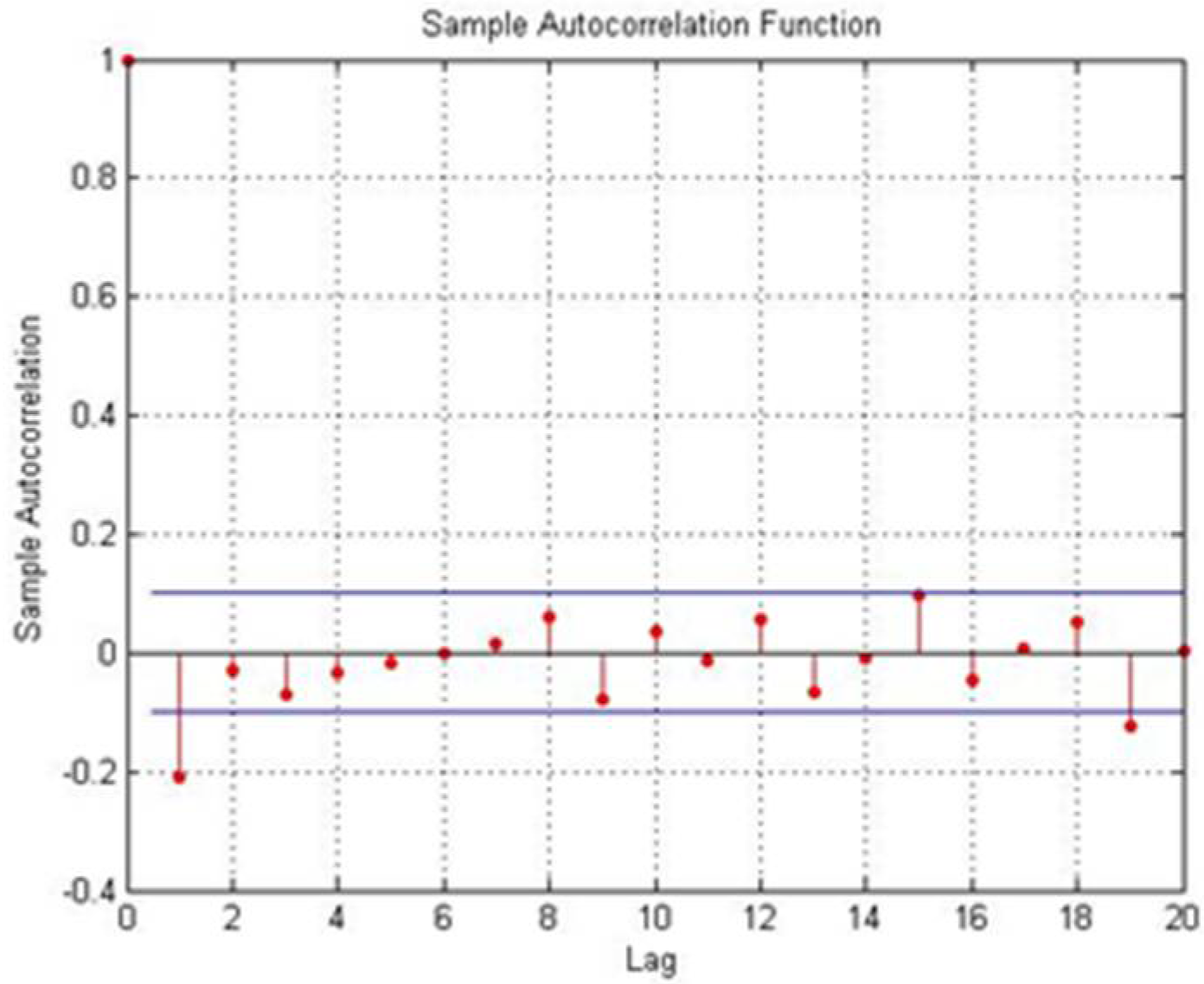
Since the minimum number of clusters is defined, we continue the iteration process until the condition (Step 7) is met. Suppose the condition is not met in the j-th iteration, in that case, we stop the iterative process and take the number of clusters from j − 1 iteration to be the maximum number of clusters. The algorithm that considers the maximum number of fuzzy states is as follows (Algorithm 3):

Algorithm 3:

Input: monitored series $\mathit{Y}(i), i=1,2,\dots ,N$

Output: maximum number of clusters mmax

Step 1. set up the initial value of M to m = mmin and k = 20

Step 2. do the fuzzy C-mean

Step 3. create interval series $[y_i^l(m),y_i^u(m)], i=1,2,\dots ,N$

Step 4. if interval series is non-stationary do d-differencing

Step 5. create center series $y_i^C,i=1,\dots ,N$

Step 6. do autocorrelation function for 20 lags $ACF(y_i^C,20)$

Step 7. if there is one and only one lag such that $ACF(y_i^C,20)>\pm 2\times standard error$,

set m+1 and go to Step 2. Otherwise stop and get $m=m_{max}$ from the previous iteration

Accordingly, the number of possible fuzzy states is defined as $\tilde{M}=[m_{min},m_{max}]$. The expected number of clusters equals the center of the interval; $E(\tilde{M})=\frac{m_{min}+m_{max}}{2}$.

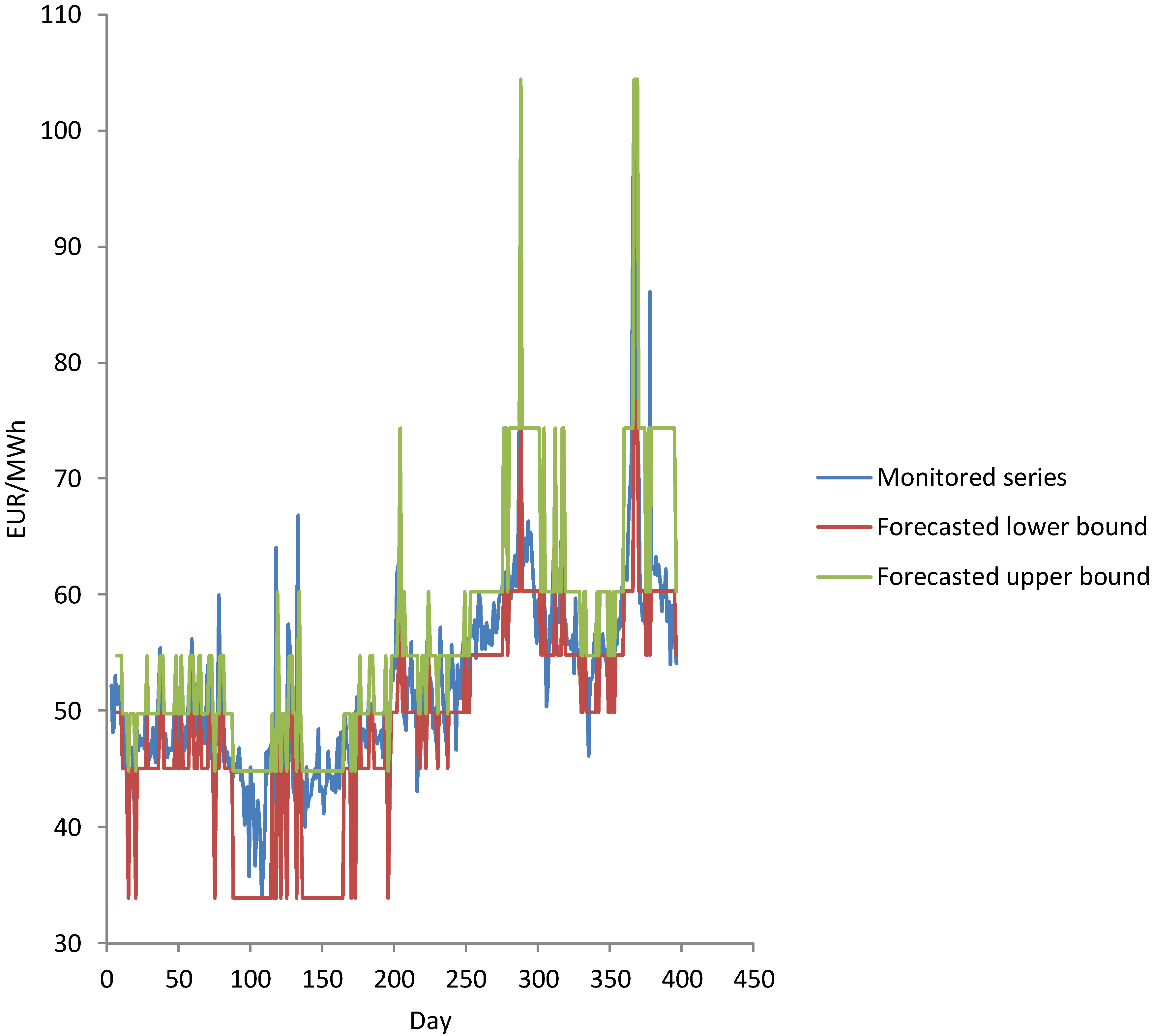
Figure 2 shows a case when the condition defined by Step 7 is not met.

Figure 2. Autocorrelation function that does not satisfy the conditions.

Algorithm 2 produces the minimum number of fuzzy states that can be used to transform a monitored series into an interval one, which can be further forecasted by the interval autoregressive process alone, while Algorithm 3 produces the maximum number of fuzzy states. In this way we can increase the flexibility of the forecasted model because any number of fuzzy states in that range can be taken for the purposes of transformation. Finally, the main aim of the proposed algorithms is to prepare a monitored series to be forecasted by the autoregressive model only.

The order of the autoregressive model (lag length) is defined according to information criteria that measure the quantity of information about the dependent variable contained in a set of regressors. In this paper we will use the Akaike information criterion (AIC) [36] and the Schwartz–Bayesian information criterion (SBIC) [37]. They are calculated by the following equations:

$$AIC=ln(\frac{{\sum }_{i=1}^N{\widehat{u}}_i^2}{N})+\frac{2k}{N},$$

(22)

$$SBIC=ln(\frac{{\sum }_{i=1}^N{\widehat{u}}_i^2}{N})+\frac{kln(N)}{N},$$

(23)

where N is the sample length; k is the total number of estimated coefficients; and ${\widehat{u}}_i$ are the residuals.

$${\widehat{u}}_i=p_i-{\widehat{s}}_i,$$

(24)

The sum of the squared residuals represents the main part of both criteria and we want to minimize it. Thus, we select the model with the smallest value of ACI or SBIC.

The absolute percentage error of the model for the i-th electricity price is calculated as follows:

$$AP{E}_i=\{\begin{array}{c}0, if p_i\in \left[{\widehat{p}}_i^l(m),{\widehat{p}}_i^u(m)\right]\\ \frac{|p_i-{\widehat{p}}_i^u(m)|+|p_i-{\widehat{p}}_i^l(m)|}{2p_i}\times 100, otherwise\end{array}.$$

(25)

To demonstrate the effectiveness of the model, the forecasted results are analyzed by the mean absolute percentage error (MAPE):

$$MAPE=\frac{1}{N}{\sum }_{i=1}^{N}AP{E}_i.$$

(26)

3. Numerical Example

In this section, we focus on the practical performance of the proposed approach. To test the efficiency of the model we used the data of daily monitored electricity price recorded by Nord Pool, N2EX Day Ahead Auction Prices [38] (Figure 3).

Figure 3. Daily monitored series of electricity price.

The set of data was divided into a training subset and validation subset. The training subset was composed of data from 1 March 2017 to 31 March 2018. We used this subset to check the confidence of the developed model. The validity subset was composed of data from 1 April 2018 to 10 April 2018, and has been used to check the validity of the model.

The results of Algorithms 2 and 3 are represented in Figure 4.

Figure 4. Autocorrelation function for: (a) three fuzzy states; (b) four fuzzy states; (c) five fuzzy states; (d) six fuzzy states; (e) seven fuzzy states.

Obviously, six fuzzy states have met the conditions of Algorithm 2 and seven fuzzy states have not met the conditions of Algorithm 3. Accordingly, the minimum number of fuzzy states is six and the maximum number of fuzzy states is six as well. Hence, the expected number of fuzzy states, i.e., clusters, is six. Fuzzy C-mean clustering algorithm has realized the following cluster center vector; C_m = [c₁, c₂, c₃, c₄, c₅, c₆] = [42.75, 47.25, 52.31, 57.26, 63.25, 90.10] and fuzzy partition matrix $U={|u_{im}|}_{396\times 6}$. Using matrix U and Equation (7) we obtained the fuzzy time series on daily monitored electricity price (see Table 1).

Table 1. Fuzzy time series of monitored series (six fuzzy states).

Year	2017	2017	2017	2017	2017	2017	2017	2017	2017	2017	2018	2018	2018
Month	3	4	5	6	7	8	9	10	11	12	1	2	3
1	s4	s2	s2	s1	s2	s2	s2	s3	s3	s5	s3	s3	s6
2	s3	s2	s3	s1	s1	s1	s2	s1	s4	s5	s4	s4	s6
3	s3	s2	s3	s1	s2	s1	s2	s2	s4	s4	s4	s4	s6
4	s2	s2	s2	s1	s4	s1	s2	s3	s3	s5	s4	s3	s5
5	s2	s3	s2	s1	s4	s1	s2	s3	s3	s5	s5	s4	s5
6	s3	s4	s2	s1	s3	s1	s2	s3	s3	s4	s4	s4	s4
7	s3	s3	s2	s1	s2	s2	s2	s2	s4	s5	s4	s4	s4
8	s3	s2	s2	s2	s1	s2	s2	s3	s4	s5	s4	s4	s4
9	s3	s2	s3	s1	s1	s1	s3	s4	s4	s5	s4	s4	s4
10	s2	s2	s3	s1	s3	s2	s2	s3	s4	s5	s5	s3	s4
11	s2	s2	s3	s1	s5	s2	s1	s3	s4	s5	s5	s3	s5
12	s2	s2	s2	s1	s2	s2	s3	s3	s3	s6	s4	s4	s4
13	s2	s2	s1	s1	s1	s2	s3	s2	s4	s5	s4	s3	s6
14	s1	s2	s2	s1	s1	s2	s3	s3	s4	s5	s4	s4	s5
15	s2	s2	s2	s1	s1	s2	s3	s2	s4	s5	s4	s3	s5
16	s2	s3	s2	s1	s1	s1	s4	s3	s4	s5	s4	s4	s5
17	s2	s2	s4	s1	s2	s2	s3	s3	s4	s5	s4	s4	s5
18	s2	s2	s3	s1	s1	s2	s5	s4	s4	s5	s4	s4	s5
19	s1	s2	s3	s2	s1	s1	s5	s3	s4	s5	s3	s4	s5
20	s2	s3	s2	s1	s1	s2	s3	s3	s4	s5	s4	s4	s5
21	s2	s2	s2	s2	s1	s3	s3	s2	s4	s5	s4	s4	s4
22	s2	s2	s2	s2	s1	s3	s3	s2	s4	s5	s4	s5	s5
23	s2	s2	s2	s1	s2	s2	s2	s3	s4	s4	s3	s5	s4
24	s2	s2	s2	s1	s1	s2	s2	s3	s4	s4	s3	s5	s5
25	s2	s2	s2	s1	s2	s2	s3	s3	s4	s4	s4	s5	s4
26	s2	s3	s1	s5	s1	s2	s3	s4	s4	s4	s4	s5	s4
27	s3	s3	s1	s2	s1	s2	s3	s3	s4	s4	s3	s5	s3
28	s2	s4	s1	s1	s1	s2	s4	s3	s4	s5	s3	s5	s4
29	s2	s2	s1	s2	s1	s3	s3	s2	s4	s4	s2		s4
30	s2	s2	s2	s2	s1	s3	s3	s3	s5	s4	s3		s4
31	s2		s2		s1	s3		s3		s3	s3		s3

The transformation of six fuzzy states into six intervals is represented by Table 2. For example, fuzzy state s1 appears 58 times in the monitored sequence. The minimum value of the electricity price for the state s1 is 33.88 EUR/MWh, which corresponds to 16 June 2017, while the maximum value is 44.78 EUR/MWh, which corresponds to 27 May 2017. In this way we defined the first interval that corresponds to fuzzy state s1. The remaining intervals are defined in the same way.

Table 2. From fuzzy state to interval.

Fuzzy State	Interval
s1	[33.88, 44.78]
s2	[45.03, 49.71]
s3	[49.82, 54.71]
s4	[54.79, 60.23]
s5	[60.30, 74.35]
s6	[76.68, 104.44]

The original time series was first transformed into an ordered fuzzy time series whereby each fuzzy state was expressed by an adequate center of cluster. After that, the ordered fuzzy time series was further transferred into an ordered interval-valued time series, where the lower bound of the interval was equal to the electricity price of the fuzzy state with a minimum value and the upper bound was equal to the electricity price of the fuzzy state with maximum value. The process of transformation is expressed by Figure 5.

Figure 5. From monitored electricity price time series to interval-valued time series: (a) fuzzy time series; (b) interval-valued time series.

The stationary nature of the time series is the main prerequisite for the application of an autoregressive process. Figure 6 shows the presence of a trend in the fuzzy time series, i.e., the series is non-stationary.

Figure 6. Trend of fuzzy time series monitored electricity price time series to interval-valued time series.

After first-order differencing of fuzzy time series and interval-valued time series, we can see that these two series became stationary series (Figure 7).

Figure 7. Stationary quality of: (a) differenced fuzzy time series and (b) differenced interval time series.

After differencing, data were prepared to be modeled by an interval autoregressive process. Hereinafter, we present the interval autoregressive process for k = 1 in detail. According to the fuzzy time series (see Table 1) starting on 1 March 2017 and ending on 31 March 2018, $\mathrm{s}4\to \mathrm{s}3\to \mathrm{s}3\to \mathrm{s}2\to \mathrm{s}2\to \dots \to \mathrm{s}4\to \mathrm{s}4\to \mathrm{s}4\to \mathrm{s}3$; we created interval time series; $[54.79,60.23]\to [49.82,54.71]\to [49.82,54.71]\to [45.03,49.71]\to [45.03,49.71]\to \dots \to [54.79,60.23]\to [54.79,60.23]\to [54.79,60.23]\to [49.82,54.71]$ (see Figure 5). Since the interval time series was non-stationary, we have done first-order differencing and obtained the following stationary series: $[-10.41,-0.08]\to [-4.89,4.89]\to [-9.68,-0.11]\to [-4.68,4.68]\dots$ (see Figure 7). The obtained stationary series was then expressed in the form of a midpoint and radius (see Table 3).

Table 3. Midpoint–radius form of interval.

Data	Interval	Midpoint	Radius
2 March 2017	$[-10.41,-0.08]$	−5.24	5.16
3 March 2017	$[-4.89, 4.89]$	0	4.89
4 March 2017	$[-9.68,-0.11]$	−4.89	4.78
$⋮$	$⋮$	$⋮$	$⋮$
31 March 2018	$[-10.41,-0.08]$	−5.24	5.16

According to the center and range method, the following matrices $\Delta A$ and $\Delta b$ are defined as follows:

$$\Delta A=\left[\begin{array}{cccc}394& 0& 0& 0\\ 0& \mathrm{13,349.34}& 0& 0\\ 0& 0& 394& 2846.09\\ 0& 0& 2846.09& \mathrm{25,842.83}\end{array}\right],$$

(27)

$$\Delta b=\left[\begin{array}{c}0\\ -4514.03\\ 2846.09\\ \mathrm{25,175.24}\end{array}\right]$$

(28)

The parameters of the interval autoregressive process are:

$$\Delta \widehat{\beta }={(\Delta {\widehat{\beta }}_0^C,\Delta {\widehat{\beta }}_1^C,\Delta {\widehat{\beta }}_0^R,\Delta {\widehat{\beta }}_1^R)}^T={(\Delta A)}^{-1}\times \Delta b=\left[\begin{array}{c}0\\ -0.338\\ 0.913\\ 0.874\end{array}\right]$$

(29)

Delta indicates that an interval autoregressive process is applied to the differenced series. The forecasting model of the midpoint–radius series is represented by the following two equations:

$$\Delta {\widehat{p}}_i^C=\Delta {\widehat{\beta }}_0^C+\Delta {\widehat{\beta }}_1^C\Delta p_{i-1}^C(m)+{\epsilon }_i^C=-0.338\Delta p_{i-1}^C(m)+{\epsilon }_i^C,$$

(30)

$$\Delta {\widehat{p}}_i^R=\Delta {\widehat{\beta }}_0^R+\Delta {\widehat{\beta }}_1^R\Delta p_{i-1}^R(m)+{\epsilon }_i^R=0.913+0.874\Delta p_{i-1}^R(m)+{\epsilon }_i^R.$$

(31)

According to Equation (19), the values of the interval differenced series is forecasted as follows:

$$\left[\Delta {\widehat{p}}_i^l,\Delta {\widehat{p}}_i^u\right]=\left[-0.338\Delta p_{i-1}^C(m)-(0.913+0.874\Delta p_{i-1}^R(m)),-0.338\Delta p_{i-1}^C(m)+(0.913+0.874\Delta p_{i-1}^R(m))\right].$$

(32)

By using Equation (20), real interval values are obtained (see Table 4).

Table 4. Forecasted interval series.

Data	Forecasted Interval	Forecasted Center
3 March 2017	$[46.16, 61.91]$	54.03
4 March 2017	$[44.63, 59.89]$	52.26
$⋮$	$⋮$	$⋮$
31 March 2018	$[49.12, 65.89]$	57.51

Now, it is necessary to inspect to what fuzzy state of M = 6 values the forecasted state (center) corresponds. Results of the application of Algorithm 1 are shown in Table 5 and Figure 8.

Table 5. Forecasted states.

Data	Forecasted Center	$\mathbf{Fuzzy} \mathbf{Partition} \mathbf{Matrix} \widehat{\mathit{U}}\mathbf{=}{\mathbf{\left|}{\widehat{\mathit{u}}}_{\mathit{i}\mathit{m}}\mathbf{\right|}}_{\mathbf{394}\mathbf{\times }\mathbf{6}}$						$\widehat{\mathit{S}}\mathbf{(}\mathit{i}\mathbf{)}$
		c1 = 42.75	c2 = 47.25	c3 = 52.31	c4 = 57.26	c5 = 63.25	c6 = 90.10
3 March 2017	54.03	0.0702	0.1167	0.4583	0.2465	0.0861	0.0219	52.31
4 March 2017	52.26	0.0044	0.0085	0.9734	0.0085	0.0038	0.0011	52.31
$⋮$	$⋮$	$⋮$	$⋮$	$⋮$	$⋮$	$⋮$	$⋮$	$⋮$
31 March 2018	57.51	0.0151	0.0217	0.0428	0.8745	0.0388	0.0068	57.26

Figure 8. Original fuzzy time series and forecasted fuzzy time series of monitored electricity price.

Absolute percentage error of the model for 4 March 2017 is:$\frac{|47.25-52.31|}{47.25}\times 100=10.71\%$. Mean absolute percentage error that regards the original fuzzy time series and forecasted fuzzy time series of monitored electricity price is 4.95%. The Akaike information criterion (AIC) for AR(1) is 3.173 and the Schwartz–Bayesian information criterion (SBIC) is 3.183. According to Equations (25) and (26), the mean absolute percentage error that regards the daily monitored electricity price and forecasted interval time series is 5.43%. Results of the model are represented by Figure 9.

Figure 9. Monitored series and forecasted interval time series.

The procedure was repeated for k = 2, 3, …, 6 and the results are shown in Table 6.

Table 6. Characteristics of the AR(k) process.

Order AR(k)	MAPE (%) Original-Forecasted States	MAPE (%) Monitored-Interval Series	AIC	SBIC
AR(1)	4.95	5.43	3.173	3.183
AR(2)	4.77	5.01	3.161	3.171
AR(3)	4.91	5.11	3.182	3.192
AR(4)	4.41	4.71	3.026	3.036
AR(5)	4.39	4.68	2.995	3.005
AR(6)	4.89	5.31	3.157	3.167

Optimal order of interval-valued autoregressive process is k = 5, and the results of the model are represented by Figure 10.

Figure 10. Plot of interval-valued autoregressive model, AR(5).

We used Algorithm 1 for period h = 1, 2, …, 10 to measure the validity of the proposed model. The obtained values are represented in Table 7 and Figure 11.

Table 7. Validity of proposed mode for h = 1, 2, …, 10.

Data	Monitored Value	Forecasted Interval	Center of Forecasted Interval	Forecasted Fuzzy State	Fuzzy Interval
1 April 2018	57.37	[49.47,68.23]	58.86	s4	[54.79,60.23]
2 April 2018	55.38	[47.04,66.70]	56.88	s4	[54.79,60.23]
3 April 2018	57.98	[47.86,66.93]	57.40	s4	[54.79,60.23]
4 April 2018	55.59	[47.84,66.92]	57.38	s4	[54.79,60.23]
5 April 2018	56.49	[48.04,67.12]	57.52	s4	[54.79,60.23]
6 April 2018	53.88	[48.22,66.93]	57.57	s4	[54.79,60.23]
7 April 2018	57.94	[48.19,67.12]	57.65	s4	[54.79,60.23]
8 April 2018	57.37	[47.89,67.08]	57.49	s4	[54.79,60.23]
9 April 2018	62.05	[47.88,67.11]	57.50	s4	[54.79,60.23]
10 April 2018	57.48	[47.82,67.16]	57.49	s4	[54.79,60.23]

Figure 11. Monitored and forecasted values of electricity price for h = 10 days.

In the two cases, the model missed the original fuzzy state within a range of ±1 state. The mean absolute percentage error for a monitored electricity price series of 10 days and forecasted fuzzy states is 1.41%.

4. Conclusions

In this paper we try to incorporate uncertainty in the electricity price forecasting model by applying interval numbers to express the price of electricity, with no intention of exploring influencing factors. We applied a fuzzy C-mean clustering algorithm to separate the data of electricity prices into an adequate number of states (clusters), with the intention of representing a price time series by a fuzzy time series, i.e., the interval state time series. The main aim of this application is to decrease the volatility of monitored series. Results that are obtained by a fuzzy C-mean algorithm were used as input to the interval-valued autoregressive forecasting model. To define the number of fuzzy states, we developed an algorithm that was based on the autocorrelation function of centers of the interval state time series. The defined number of states prepares the original data to be modeled (forecasted) by an autoregressive process only. The order of the autoregressive process is defined by Akaike and Schwartz–Bayesian information criterion. The model was tested on the real monitored electricity price series and the accuracy of the model was very high.

References

- Weron, R. Electricity price forecasting: A review of the state-of-the-art with a look into time future. Int. J. Forecast. 2014, 30, 1030–1081. [Google Scholar] [CrossRef]
- Nowotarski, J.; Weron, R. Recent advances in electricity price forecasting: A review of probabilistic forecasting. Renew. Sustain. Energy Rev. 2018, 81, 1548–1568. [Google Scholar] [CrossRef]
- Shahidehpour, M.; Yamin, H.; Li, Z. Market Operations in Electric Power Systems: Forecasting, Scheduling, and Risk Management; Wiley: Hoboken, NJ, USA, 2002; Chapter 3; pp. 57–113. [Google Scholar]
- Skantze, P.L.; Ilic, M.D. Valuation, Hedging and Speculation in Competitive Electricity Markets: A Fundamental Approach; Kluwer Academic Publishers: Dordrecht, The Netherlands, 2001. [Google Scholar]
- Dutta, G.; Mitra, K. A literature review on dynamic pricing of electricity. J. Oper. Res. Soc. 2017, 68, 1131–1145. [Google Scholar] [CrossRef]
- Aggarwal, S.K.; Saini, L.M.; Ashwani, K. Electricity price forecasting in deregulated markets: A review and evaluation. Electr. Power Energy Syst. 2009, 31, 13–22. [Google Scholar] [CrossRef]
- Chuntian, C.; Bin, L.; Shumin, M.; Xinyu, W. Mid-Term Electricity Market Clearing Price Forecasting with Sparse Data: A Case in Newly-Reformed Yunnan Electricity Market. Energies 2016, 9, 804. [Google Scholar] [CrossRef]
- Contreras, J.; Espínola, R.; Nogales, F.J.; Conejo, A.J. ARIMA Models to Predict Next-Day Electricity Prices. IEEE Trans. Power Syst. 2003, 18, 1014–1020. [Google Scholar] [CrossRef]
- Barlow, M. A diffusion model for electricity prices. Math Financ. 2002, 12, 287–298. [Google Scholar] [CrossRef]
- Fu, Y.; Li, Z. Different models and properties on LMP calculations. In Proceedings of the 2006 IEEE Power Engineering Society General Meeting, Montreal, QC, Canada, 18–22 June 2006. [Google Scholar] [CrossRef]
- Voronina, S.; Partanena, J. A Hybrid electricity price forecasting model for the Finnish electricity spot market. In Proceedings of the 32st Annual International Symposium on Forecasting, Boston, MA, USA, 24–27 June 2012. [Google Scholar]
- Aggarwal, S.K.; Saini, L.M.; Ashwani, K. Electricity Price Forecasting in Ontario Electricity Market Using Wavelet Transform in Artificial Neural Network Based Model. Int. J. Control Autom. Syst. 2008, 6, 639–650. [Google Scholar]
- Ghodsi, R.; Zakerinia, M.S. Forecasting Short Term Electricity Price Using Artificial Neural Network and Fuzzy Regression. Int. J. Acad. Res. Bus. Soc. Sci. 2012, 2, 286–293. [Google Scholar]
- Yamin, H.Y.; Shahidehpour, S.M.; Li, Z. Adaptive short-term electricity price forecasting using artificial neural networks in the restructured power markets. Int. J. Electr. Power Energy Syst. 2004, 26, 571–581. [Google Scholar] [CrossRef]
- Cerjan, M.; Matijaš, M.; Delimar, M. Dynamic Hybrid Model for Short-Term Electricity Price Forecasting. Energies 2014, 7, 3304–3318. [Google Scholar] [CrossRef]
- Esfahan, M. Neuro-fuzzy approach for short-term electricity price forecasting developed MATLAB-based software. Fuzzy Inf. Eng. 2011, 3, 339–350. [Google Scholar] [CrossRef]
- Tian, S.A.L.; Jia, L.N. Anticipating electricity prices for future needs—Implications for liberalised retail markets. Appl. Energy 2018, 212, 244–264. [Google Scholar] [CrossRef]
- Ziel, F.; Weron, R. Day-ahead electricity price forecasting with high-dimensional structures: Univariate vs. multivariate modeling frameworks. Energy Econ. 2018, 70, 396–420. [Google Scholar] [CrossRef]
- Gonzalez, J.P.; Munoz, S.R.A.; Estrella, A. Perez. Forecasting Functional Time Series with a New Hilbertian ARMAX Model: Application to Electricity Price Forecasting. IEEE Trans. Power Syst. 2018, 33, 545–556. [Google Scholar] [CrossRef]
- Nieta, A.A.S.; Gonzalez, V.; Contreras, J. Portfolio Decision of Short-Term Electricity Forecasted Prices through Stochastic Programming. Energies 2016, 9, 1069. [Google Scholar] [CrossRef]
- Neupane, B.; Woon, W.L.; Aung, Z. Ensemble Prediction Model with Expert Selection for Electricity Price Forecasting. Energies 2017, 10, 77. [Google Scholar] [CrossRef]
- Alvarez, F.M.; Troncoso, A.; Riquelme, J.C.; Riquelme, J.M. Partitioning-Clustering Techniques Applied to the Electricity Price Time Series; Yin, H., Tino, P., Corchado, E., Byrne, W., Yao, X., Eds.; IDEAL 2007. LNCS 4881; Springer: Berlin/Heidelberg, Germany, 2007; pp. 990–999. [Google Scholar]
- Safarinejadian, B.; Gharibzadeh, M.; Rakhshan, M. An optimized model of electricity price forecasting in the electricity market based on fuzzy time series. Syst. Sci. Control Eng. 2014, 2, 677–683. [Google Scholar] [CrossRef]
- Sokhanvar, K.; Karimpour, A.; Pariz, N. Electricity price forecasting using a clustering approach. In Proceedings of the 2nd IEEE International Conference on Power and Energy (PECon 08), Johor Baharu, Malaysia, 1–3 December 2008; pp. 1302–1305. [Google Scholar]
- Itaba, S.; Mori, H. A fuzzy-preconditioned GRBFN model for electricity price forecasting. Procedia Comput. Sci. 2017, 114, 441–448. [Google Scholar] [CrossRef]
- Song, Q.; Chissom, B.S. Fuzzy time series and its models. Fuzzy Sets Syst. 1993, 54, 269–277. [Google Scholar] [CrossRef]
- Sheng, T.L.; Cheng, Y.C.; Lin, S.Y. A FCM-based deterministic forecasting model for fuzzy time series. Comput. Math. Appl. 2008, 56, 3052–3063. [Google Scholar]
- Bezdek, J.C.; Enrlich, R.; Full, W. FCM: The fuzzy c-means clustering algorithm. Comput. Geosci. 1984, 10, 191–203. [Google Scholar] [CrossRef]
- Lu, Y.H.; Ma, T.H.; Yin, C.H.; Xie, X.Y.; Tian, W.; Zhong, S.M. Implementation of the Fuzzy C-Means Clustering Algorithm in Meteorogical Data. Int. J. Database Theory Appl. 2013, 6, 1–18. [Google Scholar] [CrossRef]
- Wang, X.; Wang, Y.; Wang, L. Improving fuzzy c-means clustering based on feature-weight learning. Pattern Recognit. Lett. 2004, 25, 1123–1132. [Google Scholar] [CrossRef]
- Chang, C.T.; Lai, J.Z.C.; Jeng, M.D. A fuzzy K-means clustering algorithm using cluster center displacement. J. Inf. Sci. Eng. 2011, 27, 995–1009. [Google Scholar]
- Moore, R.E.; Kearfott, R.B.; Cloud, M.J. Introduction to Interval Analysis; SIAM Press: Philadelphia, PA, USA, 2009. [Google Scholar]
- Hickey, T.; Qun, J.; Emden, M.H. Interval Arithmetic: From Principles to Implementation. J. ACM 2001, 48, 1–34. [Google Scholar] [CrossRef]
- Giordani, P. Linear Regression Analysis for Interval-Valued Data Based on the Lasso Technique. Available online: http://www.dss.uniroma1.it/en/system/files/pubblicazioni/9-RT_6_2011_Giordani.pdf (accessed on 29 April 2018).
- Neto, E.L.; Carvalho, F. Centre and range method for fitting a linear regression model to symbolic interval data. Comput. Stat. Data Anal. 2007, 52, 1500–1515. [Google Scholar] [CrossRef]
- Akaike, H. A new look at the statistical model identification. IEEE Trans. Autom. Control 1974, 19, 716–723. [Google Scholar] [CrossRef]
- Schwarz, G. Estimating the dimension of a model. Ann. Stat. 1978, 6, 461–464. [Google Scholar] [CrossRef]
- N2EX Day Ahead Auction Prices. Available online: https://www.nordpoolgroup.com/Market-data1/GB/Auction-prices/UK/Daily/?view=table (accessed on 16 March 2018).
© 2018 by the authors. Licensee MDPI, Basel, Switzerland. This article is an open access article distributed under the terms and conditions of the Creative Commons Attribution (CC BY) license (http://creativecommons.org/licenses/by/4.0/).