An Analytical Model for the Effect of Vertical Wind Veer on Wind Turbine Wakes

Abstract

In this study, an analytical wake model for predicting the mean velocity field downstream of a wind turbine under veering incoming wind is systematically derived and validated. The new model, which is an extended version of the one introduced by Bastankhah and Porté-Agel, is based upon the application of mass conservation and momentum theorem and considering a skewed Gaussian distribution for the wake velocity deficit. Particularly, using a skewed (instead of axisymmetric) Gaussian shape allows accounting for the lateral shear in the incoming wind induced by the Coriolis force. This analytical wake model requires only the wake expansion rate as an input parameter to predict the mean wake flow downstream. The performance of the proposed model is assessed using the large-eddy simulation (LES) data of a full-scale wind turbine wake under the stably stratified condition. The results show that the proposed model is capable of predicting the skewed structure of the wake downwind of the turbine, and its prediction for the wake velocity deficit is in good agreement with the high-fidelity simulation data.

1. Introduction

The presence of the Coriolis force in the atmospheric boundary layer (ABL) causes the wind direction to vary with height and results in a lateral wind shear besides the vertical one. Much work, including numerical simulations and field-scale measurements [1,2,3,4,5,6,7,8,9], has been done recently to unravel the impact of lateral wind shear (also known as vertical wind veer) on the aerodynamics of wind turbine wakes. All these studies highlighted that, for the large utility-scale wind turbines, the impact of the lateral wind shear cannot be ignored. Specifically, they showed that the directionally sheared inflow induces a skewed structure in the spatial distribution of the wake which can potentially affect the efficiency of the downstream wind turbines [10,11,12,13].

In addition to the high-fidelity numerical and experimental techniques, it is of particular interest for wind energy applications to have low-order, physically-based models to predict the wind turbine wakes under different atmospheric regimes. Among the previous theoretical developments for wind turbine wakes, one can mention the Jensen model [14] and the Bastankhah and Porté-Agel model (also known as the Gaussian wake model) [15]. The former, which is based on assuming a top-hat distribution for the wake velocity deficit, is widely used in the wind energy community for the design and layout optimization of wind farms. The later one, however, is based upon considering an axisymmetric Gaussian distribution for the wake velocity deficit and was found to yield a more accurate prediction, especially in the partial wake condition, with respect to the top-hat model [16]. However, the existing analytical wake models are restricted to the unidirectional inflow and are unable to account for the effect of lateral wind shear associated with the Coriolis force. Since all wind turbines operating in the ABL are exposed to the Coriolis effect, developing reliable low-order models for wake flow prediction under directionally sheared inflow is valuable and is the focus of the present work.

The objective of this study is to develop and validate an analytical model for prediction of wind turbine wakes under directionally sheared incoming wind. The proposed model is based upon the application of mass conservation and momentum theorem (as in Bastankhah and Porté-Agel model [15]) and assuming a skewed Gaussian distribution for the wake velocity deficit. In order to examine the performance of the proposed model, the results from the large-eddy simulation (LES) of a full-scale wind turbine wake in the stably stratified condition are used. The LES framework and the simulation results are described in Section 2. In Section 3, the derivation of the analytical wake model is presented, and the performance of the proposed model is assessed using the LES data. A summary and concluding remarks are given in Section 4.

2. Large-Eddy Simulation Framework

2.1. LES Governing Equations

The LES framework utilized in this study, which has been employed in previous wind-energy research studies (e.g., [17,18,19,20,21]), is based upon the filtered incompressible Navier-Stokes equations, including the Coriolis and buoyancy effects, and the filtered transport equation for the potential temperature,

$$\begin{array}{c}{\partial }_i{\tilde{u}}_i=0,\hfill \\ {\partial }_t{\tilde{u}}_i+{\partial }_j\left({\tilde{u}}_i{\tilde{u}}_j\right)=-{\partial }_i\tilde{p}+{\partial }_j\left(\nu {\partial }_j{\tilde{u}}_i\right)-{\partial }_j{\tau }_{ij}+{\delta }_{i3}\beta (\tilde{\theta }-\langle \tilde{\theta }\rangle )+f_c{\epsilon }_{ij3}{\tilde{u}}_j-f_i/\rho ,\hfill \\ {\partial }_t\tilde{\theta }+{\partial }_i\left({\tilde{u}}_i\tilde{\theta }\right)={\partial }_i\left(\kappa {\partial }_i\tilde{\theta }\right)-{\partial }_i{q}_i,\hfill \end{array}$$

(1)

where t represents the time, the tilde a spatial filtering, ${\tilde{u}}_i$ the resolved velocity component in the ith direction (where $i=1,2,3$ refers to the streamwise (x), lateral (y) and wall-normal (z) directions, respectively), $\tilde{\theta }$ the resolved potential temperature, $\tilde{p}$ the kinematic pressure, $\rho$ the fluid density, $\nu$ the kinematic viscosity, $\kappa$ the thermal diffusivity, $f_c$ the Coriolis parameter, and ${\epsilon }_{ijk}$ the alternating unit tensor. ${\tau }_{ij}=\widetilde{u_i{u}_j}-{\tilde{u}}_i{\tilde{u}}_j$ and $q_i=\widetilde{u_i\theta }-{\tilde{u}}_i\tilde{\theta }$ denote the subfilter stress tensor and heat-flux vector, respectively. To account for the buoyancy effects in the momentum transport equations, the Boussinesq approximation following [22] is used. $\beta =g/{\theta }_0$ indicates the buoyancy parameter, where ${\theta }_0$ is the reference potential temperature, and g is the gravitational acceleration. The angled brackets show a horizontal average, and ${\delta }_{ij}$ is the Kronecker delta. $f_i$ is a body force to model the influence of the wind turbine on the flow field. Here, the standard actuator-disk approach is employed to model the turbine-induced forces [23,24,25], and the subfilter turbulent fluxes are parametrized via the Lagrangian scale-dependent dynamic approach [26]. Detailed description of the numerical method of the LES framework can be found in [27,28,29,30,31,32,33].

2.2. Numerical Setup

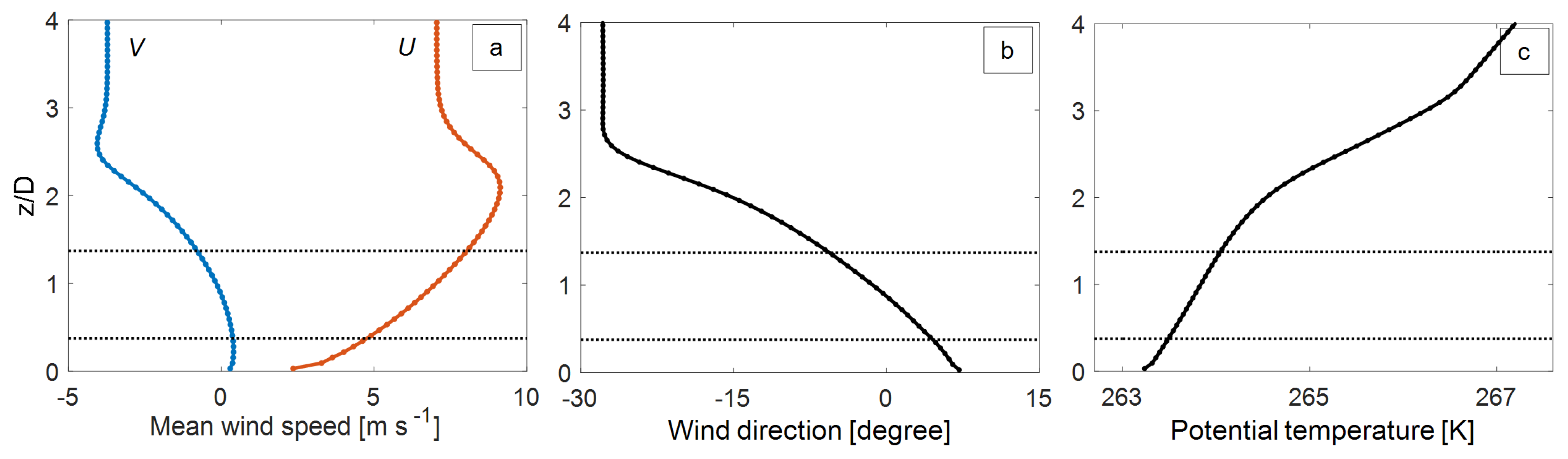
To provide the inflow for the wind turbine wake simulation, a precursor technique is used in which a stably stratified ABL without the wind turbine is simulated. Note that the impact of vertical wind veer is stronger under the stably stratified regimes due to the shallower boundary-layer depth [34]. In the present work, we simulate the standard GABLS (GEWEX Atmospheric Boundary Layer Study) case which represents a moderately stable boundary layer [35].

The domain size is 1920 m $\times 960$ m $\times 475$ m, and it is discretized into $192\times 96\times 96$ grid-points in the $x,y,z$ directions, respectively. To drive the boundary layer, a uniform geostrophic wind of 8 m·s${}^{-1}$ is applied. The latitude is set to ${73}^{\circ }$ N with a Coriolis parameter of $f_c=1.39\times {10}^{-4}$ rad·s${}^{-1}$. The simulation is initialized with a uniform streamwise velocity of 8 m·s${}^{-1}$, and the spanwise and wall-normal velocity components are set to zero. The initial potential temperature is set to 265 K in the lowest 100 m, and then increases linearly with a constant lapse rate of 10 K·km${}^{-1}$. The surface cooling rate is set to $-0.25$ K·h${}^{-1}$ during the nine hours of the simulation. ${\theta }_0$ in the buoyancy term is set to $263.5$ K. The aerodynamic surface roughness for the heat and momentum is set to $0.1$ m. The surface fluxes are computed using the Monin-Obukhov similarity theory including the stability correction [29,36,37]. A wind direction controller is also utilized in order to have the turbine axes aligned with the mean wind direction. Through this method, the geostrophic wind is gradually adjusted by adding a source term to the momentum conservation equations [7,10,25,38]. Since the simulation reaches a quasi-steady state during the last hour of the simulation (i.e., 8–9 h) [35], the instantaneous fields of the velocity and temperature during this time are stored and used as the inflow in the simulation of the wind turbine wake. In the wake flow simulation, a wind turbine with a rotor diameter (D) of 80 m and a hub height ($z_{hub}$) of 70 m is immersed in the flow. The thrust coefficient of the turbine is set to $0.75$ as in the previous studies [25,39,40]. Note that a similar case with a smaller computational domain was used in [7] to investigate the impact of wind veer on the wake meandering and turbulence statistics downstream of the turbine.

2.3. LES Results

Figure 1a–c illustrates the mean profiles of the horizontal wind components, wind direction and potential temperature of the simulated ABL flow in the absence of wind turbine. As seen in this figure, the wind direction varies with height due to the presence of the Coriolis effect. Note that, as a result of the wind direction controller, the mean wind direction at the hub height is almost zero throughout the simulation. The mean wind velocity at the hub-height level ($U_{hub}$) is about $6.64$ m·s${}^{-1}$, and the turbulence level is about 5%. The turbulence level is defined as $\sqrt{2k/3}/U_{hub}$, where k denotes the resolved turbulent kinetic energy.

Figure 2 shows the contours of the normalized velocity deficit ($\Delta U/U_{hub}$) in the $y-z$ planes at different distance downstream of the turbine (i.e., $x/D=$ 3, 5, 7, and 10). The mean velocity deficit is defined as $\Delta U=U_{in}-U$, where $U_{in}$ is the mean streamwise inflow velocity. As can be visually acknowledged, due to the lateral component of the incoming wind, the wake is skewed as it is advected downstream. This is a well-known phenomenon and has been shown in several field-scale and numerical investigations of wake flow in the stable regimes [1,2,3,4,5,6,7,8,10].

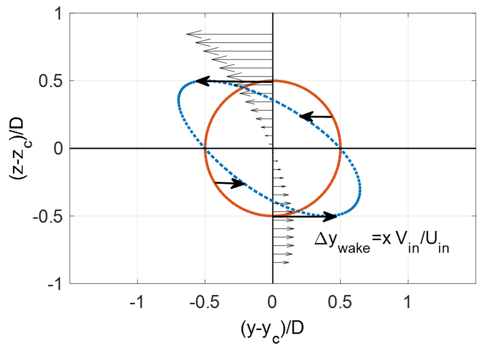
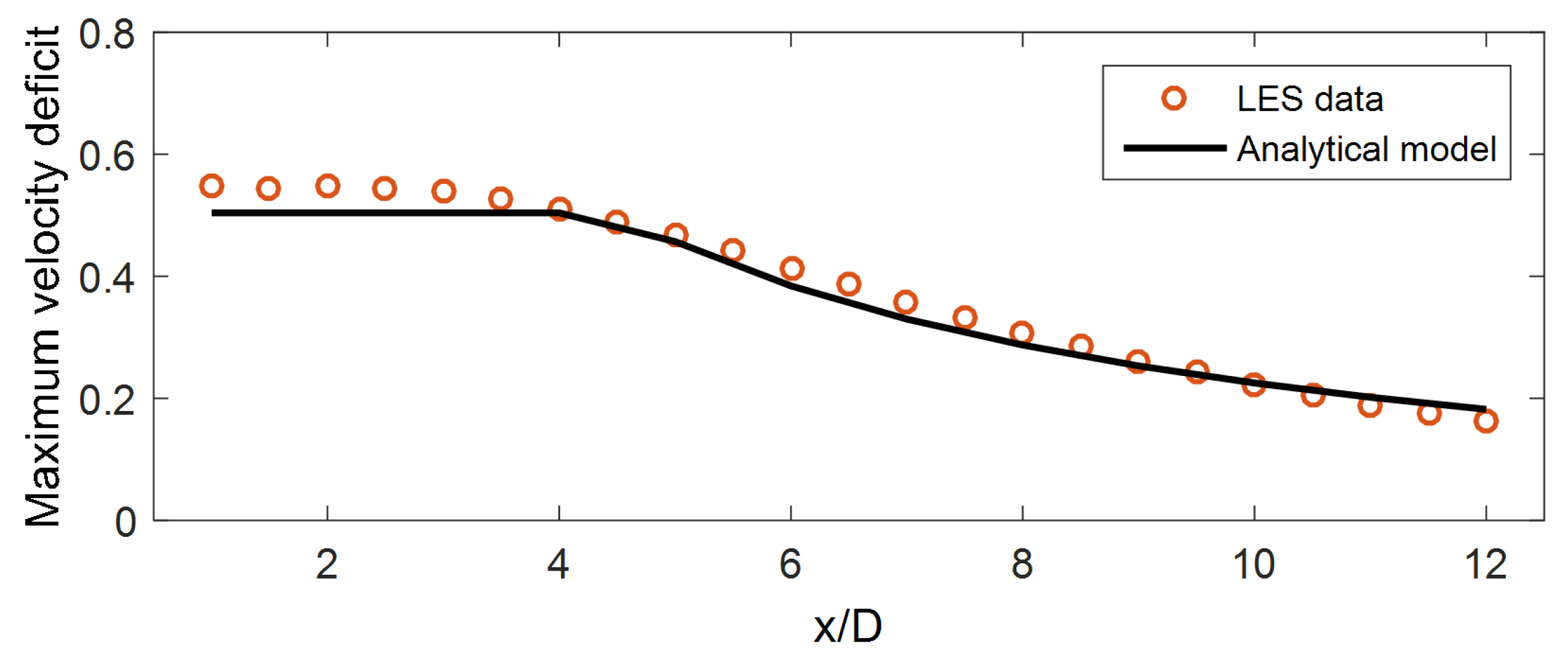
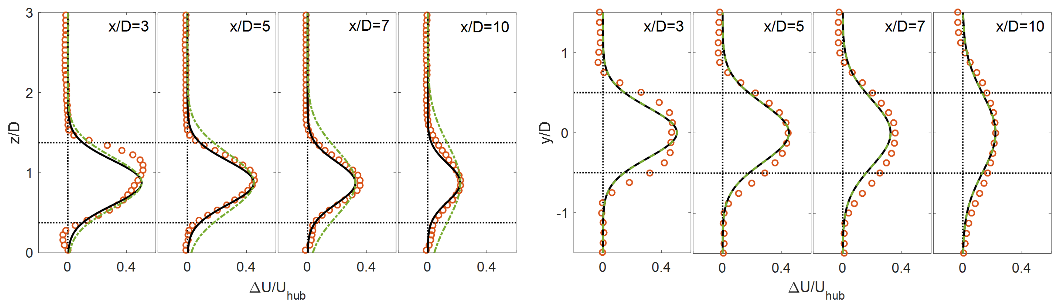
3. Analytical Wake Model

In the absence of vertical wind veer, the previous numerical and experimental investigations (e.g., [15,41,42,43,44,45]) showed that the normalized velocity deficit in the wind turbine wake follows a self-similar Gaussian shape. Taking advantage of this important observation, Bastankhah and Porté-Agel [15] developed a low-order model to estimate the mean velocity field in the wake region. In their model, which satisfied the mass and momentum conversations, an axisymmetric self-similar Gaussian shape for the wake velocity deficit was considered. Later, Abkar and Porté-Agel [42] and Xie and Archer [43] modified the axisymmetric Gaussian model by assuming an elliptical Gaussian shape for the wake velocity deficit to include the different lateral and wall-normal wake growth rates caused by the presence of the ground as well as the nonuniform incoming wind. The Gaussian wake model has been validated against the experimental data (wind-tunnel and field-scale measurements) as well as the high-resolution eddy-resolving simulation data of wind turbine wakes under neutrally and thermally stratified regimes. More details on the derivation of the Gaussian wake model can be found in [15]. Note that the previous Gaussian wake models have been limited to the unidirectional inflow in which the impact of lateral wind shear is ignored.

As shown in Figure 2, the wake is skewed under veering incoming wind owing to the lateral component of the velocity in the incoming wind. Hence, assuming an axisymmetric Gaussian distribution for the velocity deficit, as used in the previous analytical wake model, is not valid anymore. To address this issue, we hypothesize that the mean wake flow can be modeled by considering a skewed Gaussian shape for the velocity deficit downstream of the turbine. Specifically, using a skewed, instead of axisymmetric, Gaussian shape accounts for the lateral wind shear in the incoming wind. The skewness of the wake is linked to the incoming wind characteristics and, in particular, it is related to the strength of the vertical wind veer. Figure 3 shows a schematic of the wake subjected to a directionally sheared inflow. The displacement of the wake in the lateral direction at each x downstream can be estimated using the inflow characteristics as

$$\Delta y_{wake}\approx V_{in}\Delta t,$$

(2)

where $V_{in}$ is the mean lateral inflow velocity, and $\Delta t$ is the travel time of the airflow from the turbine to the downwind location at x which can be estimated as

$$\Delta t\approx x/U_{in}.$$

(3)

Inserting (3) in (2) leads to the following equation for the lateral displacement of wake at each x downstream,

$$\Delta y_{wake}\approx x\frac{V_{in}}{U_{in}}=xtan\left({\alpha }_{in}\right).$$

(4)

where ${\alpha }_{in}$ is the incoming wind angle and is varying with height. Note that if the information about the wind direction over the turbine rotor is available, the incoming wind angle in the proposed wake model can be estimated as

$${\alpha }_{in}\approx \left(\frac{{\alpha }_{tt}-{\alpha }_{bt}}{D}\right)\left(z-z_{hub}\right),$$

(5)

where ${\alpha }_{tt}$ and ${\alpha }_{bt}$ are the incoming wind angle at the top-tip and the bottom-tip levels, respectively.

By knowing the lateral displacement of the wake at each x downstream, the normalized velocity deficit in the wake region can be expressed as,

$$\frac{\Delta U}{U_{hub}}=\frac{U_{in}-U}{U_{hub}}=\frac{\Delta U_{\max }}{U_{hub}}\times exp\left(-\frac{1}{2}\left[{\left(\frac{y+xtan\left({\alpha }_{in}\right)}{{\sigma }_y}\right)}^2+{\left(\frac{z-z_{hub}}{{\sigma }_z}\right)}^2\right]\right),$$

(6)

where ${\sigma }_y$ and ${\sigma }_z$ are the standard deviation of the velocity deficit profiles with a Gaussian shape, in the absence of vertical wind veer, in the lateral and wall-normal directions, respectively. The maximum velocity deficit in the self-similar region of the wake can be computed as [15,42],

$$\frac{\Delta U_{\max }}{U_{hub}}=\left(1-\sqrt{1-\frac{C_t}{8\left({\sigma }_y/D\right)\left({\sigma }_z/D\right)}}\right),$$

(7)

where $C_t$ is the turbine thrust coefficient. Note that the analytical solution in (7) may diverge in the near wake region where the wake does reach into a full self-similar Gaussian shape. However, using the one-dimensional momentum theory, it can be shown that the normalized maximum velocity deficit should not exceed $2a$, where a refers to the axial induction factor and is related to the thrust coefficient as [46]

$$a=\frac{1-\sqrt{1-C_t}}{2}.$$

(8)

Hence, in the region close to the turbine, where (7) either diverges or yields values greater that $2a$, the normalized maximum velocity deficit is set to $2a$.

Similar to the previous studies [15,42,43,44,47,48], it is assumed that, under turbulent inflow conditions, ${\sigma }_y$ and ${\sigma }_z$ are expanded approximately linearly with downwind distance as

$$\begin{array}{c}\hfill {\sigma }_y=k_y^{*}x+ϵD,{\sigma }_z=k_z^{*}x+ϵD,\end{array}$$

(9)

where $k_y^{*}$ and $k_z^{*}$ denote the wake growth rate in the lateral and wall-normal directions, respectively. Here, $ϵ$ is a non-dimensional parameter related to the standard deviation of the wake as x approaches zero and can be modeled as [15,49]

$$ϵ=0.2\sqrt{\beta },\mathrm{where}\beta =\frac{1}{2}\frac{1+\sqrt{1-C_t}}{\sqrt{1-C_t}}.$$

(10)

In this study, in order to minimize the number of input parameters, similar wake growth rates are assumed in the lateral and wall-normal directions, i.e., $k_y^{*}=k_z^{*}=k^{*}$. Here, we adopt $k^{*}\approx 0.024$ for the wake expansion rate, corresponding the incoming turbulence level of 5%, that fits the data best. This value is consistent with the ones suggested in the previous studies for the turbine wake prediction under different atmospheric regimes [10,16,42].

The variation of the normalized maximum velocity deficit, downstream of the turbine, obtained from the analytical model is presented in Figure 4, and it is compared with the one obtained from the LES simulation. As shown in this figure, the proposed model can predict the maximum wake velocity deficit downstream of the turbine reasonably well. Note that, as also experimentally shown [44], in the potential core of the wake developed immediately behind the turbine, the velocity deficit has an approximately uniform distribution. After a certain distance downstream, the potential core of the wake fully disappears, and the maximum velocity deficit starts to decrease. A similar trend is found here where the maximum velocity deficit is approximately constant in the region close to the turbine, and then decreases with the downwind distance.

A quantitative comparison between the proposed wake model and the high-fidelity simulation data are provided in Figure 5. The results obtained from the non-skewed Gaussian wake model [15] are also provided for comparison. As can be realized, the proposed model is capable of predicting the velocity deficit distribution with downwind distance with a good accuracy. It is also observed that the accuracy of the non-skewed Gaussian wake model, in the prediction of the wake velocity, decreases in the vertical direction since it ignores the effect of vertical wind veer. Note that there is a slight discrepancy between the proposed wake model and the simulation data in the region very close to the turbine (i.e., $x/D=3$). This is mainly because, as mentioned before, the velocity deficit does not reach into a full self-similar Gaussian distribution in the region immediately behind the turbine.

Figure 6 displays the contours of the predicted velocity deficit from the proposed analytical wake model as well as the non-skewed Gaussian wake model [15] in the $y-z$ planes at different distances (i.e., $x/D=$ 3, 5, 7, and 10) downstream of the turbine. It can be visually acknowledged that there is an acceptable agreement between the the results obtained from the proposed wake model and the LES simulation (shown in Figure 2). In particular, unlike the non-skewed wake model, the proposed model can thoroughly capture the skewed structure of the wake caused by the vertical wind veer.

4. Conclusions

The present work aims to develop an analytical model for prediction of the wake velocity distribution downstream of the wind turbine under veering inflow conditions. The proposed model, which is an extended version of the one introduced by Bastankhah and Porté-Agel [15], satisfies the mass and momentum conservation and assumes a skewed Gaussian shape for the wake velocity deficit. Through this approach, the velocity deficit in the wake region can be model as

$$\frac{\Delta U}{U_{hub}}=\frac{\Delta U_{\max }}{U_{hub}}\times exp\left(-\frac{1}{2}\left[{\left(\frac{y+xtan\left({\alpha }_{in}\right)}{k_y^{*}x+ϵD}\right)}^2+{\left(\frac{z-z_{hub}}{k_z^{*}x+ϵD}\right)}^2\right]\right),$$

(11)

where $k_y^{*}$ and $k_z^{*}$ are the growth rates of the wake in the lateral and vertical directions, ${\alpha }_{in}$ is the incoming wind angle, and $\Delta U_{\max }/U_{hub}$ and $ϵ$ are obtained from (7) and (10), respectively. The key assumption in this model, which is consistent with previous numerical and experimental observations, is that the turbulent wake is expanded approximately linearly as it is transported downstream. Besides the information about the turbine thrust coefficient and the inflow characteristics (i.e., wind speed and wind direction), this model requires only the wake growth rate to predict the velocity distribution downstream of the turbine, and that can be estimated as a function of the incoming turbulence level. The performance of the proposed analytical wake model is assessed with the LES data of a full-scale wind turbine wake under the stably stratified condition. It is found that the proposed low-order wake model yields accurate prediction for the wake velocity deficit, and its prediction is in good agreement with the high-fidelity simulation data. It is also shown that, unlike the previous analytical wake models (e.g., the top-hat and the axisymmetric Gaussian wake models), the proposed model can thoroughly capture the skewed structure of the wake caused by the vertical wind veer.

Finally, it should be noted that wind turbines might operate in yawed conditions as well as in complex terrain, in addition to different atmospheric turbulence regimes. Future research is required to study the effect of vertical wind veer on wind turbine wakes in those conditions.

References

1. Magnusson, M.; Smedman, A.S. Influence of atmospheric stability on wind turbine wakes. Wind Eng. 1994, 18, 139–152. [Google Scholar]
2. Lu, H.; Porté-Agel, F. Large-eddy simulation of a very large wind farm in a stable atmospheric boundary layer. Phys. Fluids 2011, 23, 065101. [Google Scholar] [CrossRef]
3. Mirocha, J.D.; Rajewski, D.A.; Marjanovic, N.; Lundquist, J.K.; Kosović, B.; Draxl, C.; Churchfield, M.J. Investigating wind turbine impacts on near-wake flow using profiling lidar data and large-eddy simulations with an actuator disk model. J. Renew. Sustain. Energy 2015, 7, 043143. [Google Scholar] [CrossRef] [Green Version]
4. Bhaganagar, K.; Debnath, M. The effects of mean atmospheric forcings of the stable atmospheric boundary layer on wind turbine wake. J. Renew. Sustain. Energy 2015, 7, 013124. [Google Scholar] [CrossRef]
5. Vollmer, L.; van Dooren, M.; Trabucchi, D.; Schneemann, J.; Steinfeld, G.; Witha, B.; Trujillo, J.; Kühn, M. First comparison of LES of an offshore wind turbine wake with dual-Doppler lidar measurements in a German offshore wind farm. J. Phys. Conf. Ser. 2015, 625, 012001. [Google Scholar] [CrossRef] [Green Version]
6. Lundquist, J.; Churchfield, M.; Lee, S.; Clifton, A. Quantifying error of lidar and sodar Doppler beam swinging measurements of wind turbine wakes using computational fluid dynamics. Atmos. Meas. Tech. 2015, 8, 907–920. [Google Scholar] [CrossRef] [Green Version]
7. Abkar, M.; Porté-Agel, F. Influence of the Coriolis force on the structure and evolution of wind turbine wakes. Phys. Rev. Fluids 2016, 1, 063701. [Google Scholar] [CrossRef]
8. Bromm, M.; Vollmer, L.; Kühn, M. Numerical investigation of wind turbine wake development in directionally sheared inflow. Wind Energy 2017, 20, 381–395. [Google Scholar] [CrossRef]
9. Howland, M.F.; Ghate, A.S.; Lele, S.K. Influence of the horizontal component of Earth’s rotation on wind turbine wakes. J. Phys. Conf. Ser. 2018, 1037, 072003. [Google Scholar] [CrossRef]
10. Abkar, M.; Sharifi, A.; Porté-Agel, F. Wake flow in a wind farm during a diurnal cycle. J. Turbul. 2016, 17, 420–441. [Google Scholar] [CrossRef]
11. Allaerts, D.; Meyers, J. Effect of inversion-layer height and Coriolis forces on developing wind-farm boundary layers. In Proceedings of the 34th Wind Energy Symposium, San Diego, CA, USA, 4–8 January 2016; p. 1989. [Google Scholar]
12. van der Laan, M.P.; Sørensen, N.N. Why the Coriolis force turns a wind farm wake clockwise in the Northern Hemisphere. Wind Energy Sci. 2017, 2, 285. [Google Scholar] [CrossRef]
13. Xie, S.; Archer, C.L. A Numerical Study of Wind-Turbine Wakes for Three Atmospheric Stability Conditions. Bound. Lay. Meteorol. 2017, 165, 87–112. [Google Scholar] [CrossRef]
14. Jensen, N. A Note on Wind Turbine Interaction; Technical Report Ris–M–2411; Roskilde National Laboratory: Roskilde, Denmark, 1983. [Google Scholar]
15. Bastankhah, M.; Porté-Agel, F. A new analytical model for wind-turbine wakes. Renew. Energy 2014, 70, 116–123. [Google Scholar] [CrossRef]
16. Niayifar, A.; Porté-Agel, F. Analytical modeling of wind farms: A new approach for power prediction. Energies 2016, 9, 741. [Google Scholar] [CrossRef]
17. Porté-Agel, F.; Wu, Y.T.; Lu, H.; Conzemius, R.J. Large-eddy simulation of atmospheric boundary layer flow through wind turbines and wind farms. J. Wind Eng. Ind. Aerodyn. 2011, 99, 154–168. [Google Scholar] [CrossRef]
18. Wu, Y.T.; Porté-Agel, F. Simulation of Turbulent Flow Inside and Above Wind Farms: Model Validation and Layout Effects. Bound. Lay. Meteorol. 2013, 146, 181–205. [Google Scholar] [CrossRef]
19. Abkar, M.; Porté-Agel, F. The Effect of Free-Atmosphere Stratification on Boundary-Layer Flow and Power Output from Very Large Wind Farms. Energies 2013, 6, 2338–2361. [Google Scholar] [CrossRef] [Green Version]
20. Abkar, M.; Porté-Agel, F. Mean and turbulent kinetic energy budgets inside and above very large wind farms under conventionally-neutral condition. Renew. Energy 2014, 70, 142–152. [Google Scholar] [CrossRef]
21. Wu, Y.T.; Porté-Agel, F. Modeling turbine wakes and power losses within a wind farm using LES: An application to the Horns Rev offshore wind farm. Renew. Energy 2015, 75, 945–955. [Google Scholar] [CrossRef]
22. Deardorff, J.W. Three-dimensional numerical study of the height and mean structure of a heated planetary boundary layer. Bound. Lay. Meteorol. 1974, 7, 81–106. [Google Scholar] [CrossRef]
23. Meyers, J.; Meneveau, C. Large Eddy Simulations of Large Wind-Turbine Arrays in the Atmospheric Boundary Layer. In Proceedings of the 48th AIAA Aerospace Sciences Meeting Including the New Horizons Forum and Aerospace Exposition, Orlando, FL, USA, 4–7 January 2010. [Google Scholar]
24. Wu, Y.T.; Porté-Agel, F. Large-Eddy Simulation of Wind-Turbine Wakes: Evaluation of Turbine Parametrisations. Bound. Lay. Meteorol. 2011, 138, 345–366. [Google Scholar] [CrossRef]
25. Abkar, M.; Porté-Agel, F. A new wind-farm parameterization for large-scale atmospheric models. J. Renew. Sustain. Energy 2015, 7, 013121. [Google Scholar] [CrossRef]
26. Stoll, R.; Porté-Agel, F. Dynamic subgrid-scale models for momentum and scalar fluxes in large-eddy simulations of neutrally stratified atmospheric boundary layers over heterogeneous terrain. Water Resour. Res. 2006, 42, W01409. [Google Scholar] [CrossRef]
27. Porté-Agel, F.; Meneveau, C.; Parlange, M.B. A Scale-Dependent Dynamic Model for Large-Eddy Simulation: Application to a Neutral Atmospheric Boundary Layer. J. Fluid Mech. 2000, 415, 261–284. [Google Scholar] [CrossRef]
28. Porté-Agel, F. A scale-dependent dynamic model for scalar transport in large-eddy simulations of the atmospheric boundary layer. Bound. Lay. Meteorol. 2004, 112, 81–105. [Google Scholar] [CrossRef]
29. Stoll, R.; Porté-Agel, F. Large-eddy simulation of the stable atmospheric boundary layer using dynamic models with different averaging schemes. Bound. Lay. Meteorol. 2008, 126, 1–28. [Google Scholar] [CrossRef]
30. Abkar, M.; Porté-Agel, F. A new boundary condition for large-eddy simulation of boundary-layer flow over surface roughness transitions. J. Turbul. 2012, 13, 1–18. [Google Scholar] [CrossRef]
31. Abkar, M.; Bae, H.; Moin, P. Minimum-dissipation scalar transport model for large-eddy simulation of turbulent flows. Phys. Rev. Fluids 2016, 1, 041701. [Google Scholar] [CrossRef]
32. Abkar, M.; Moin, P. Large-Eddy Simulation of Thermally Stratified Atmospheric Boundary-Layer Flow Using a Minimum Dissipation Model. Bound. Lay. Meteorol. 2017, 165, 405–419. [Google Scholar] [CrossRef]
33. Yang, X.I.; Abkar, M. A hierarchical random additive model for passive scalars in wall-bounded flows at high Reynolds numbers. J. Fluid Mech. 2018, 842, 354–380. [Google Scholar] [CrossRef]
34. Esau, I.N.; Zilitinkevich, S.S. Universal dependences between turbulent and mean flow parameters instably and neutrally stratified Planetary Boundary Layers. Nonlin. Process. Geophys. 2006, 13, 135–144. [Google Scholar] [CrossRef] [Green Version]
35. Beare, R.J.; MacVean, M.K.; Holtslag, A.A.M.; Cuxart, J.; Esau, I.; Golaz, J.C.; Jimenez, M.A.; Khairoutdinov, M.; Kosovic, B.; Lewellen, D.; et al. An intercomparison of large-eddy simulations of the stable boundary layer. Bound. Lay. Meteorol. 2006, 118, 247–272. [Google Scholar] [CrossRef]
36. Moeng, C. A large-eddy simulation model for the study of planetary boundary-layer turbulence. J. Atmos. Sci. 1984, 46, 2311–2330. [Google Scholar] [CrossRef]
37. Basu, S.; Porté-Agel, F. Large-eddy simulation of stably stratified atmospheric boundary layer turbulence: A scale-dependent dynamic modeling approach. J. Atmos. Sci. 2006, 63, 2074–2091. [Google Scholar] [CrossRef]
38. Sescu, A.; Meneveau, C. A control algorithm for statistically stationary large-eddy simulations of thermally stratified boundary layers. Q. J. R. Meteorol. Soc. 2014, 140, 2017–2022. [Google Scholar] [CrossRef]
39. Jimenez, A.; Crespo, A.; Migoya, E.; Garcia, J. Advances in large-eddy simulation of a wind turbine wake. J. Phys. Conf. Ser. 2007, 75, 012041. [Google Scholar] [CrossRef] [Green Version]
40. Calaf, M.; Meneveau, C.; Meyers, J. Large eddy simulation study of fully developed wind turbine array boundary layers. Phys. Fluids 2010, 22, 015110. [Google Scholar] [CrossRef]
41. Chamorro, L.; Porté-Agel, F. A wind-tunnel investigation of wind-turbine wakes: Boundary-layer turbulence effects. Bound. Lay. Meteorol. 2009, 132, 129–149. [Google Scholar] [CrossRef]
42. Abkar, M.; Porté-Agel, F. Influence of atmospheric stability on wind turbine wakes: A large-eddy simulation study. Phys. Fluids 2015, 27, 035104. [Google Scholar] [CrossRef]
43. Xie, S.; Archer, C. Self-similarity and turbulence characteristics of wind turbine wakes via large-eddy simulation. Wind Energy 2015, 18, 1815–1838. [Google Scholar] [CrossRef]
44. Bastankhah, M.; Porté-Agel, F. Experimental and theoretical study of wind turbine wakes in yawed conditions. J. Fluid Mech 2016, 806, 506–541. [Google Scholar] [CrossRef]
45. Ishihara, T.; Qian, G.W. A new Gaussian-based analytical wake model for wind turbines considering ambient turbulence intensities and thrust coefficient effects. J. Wind Eng. Ind. Aerodyn. 2018, 177, 275–292. [Google Scholar] [CrossRef]
46. Manwell, J.F.; McGowan, J.G.; Rogers, A.L. Wind Energy Explained: Theory, Design and Application; John Wiley & Sons: Hoboken, NJ, USA, 2010. [Google Scholar]
47. Abkar, M.; Dabiri, J.O. Self-similarity and flow characteristics of vertical-axis wind turbine wakes: An LES study. J. Turbul. 2017, 18, 373–389. [Google Scholar] [CrossRef]
48. Carbajo Fuertes, F.; Markfort, C.D.; Porté-Agel, F. Wind Turbine Wake Characterization with Nacelle-Mounted Wind Lidars for Analytical Wake Model Validation. Remote Sens. 2018, 10, 668. [Google Scholar] [CrossRef]
49. Burton, T.; Sharpe, D.; Jenkins, N.; Bossanyi, E. Wind Energy Handbook; Wiley: New York, NY, USA, 2001. [Google Scholar]
Figure 1. Mean profiles of (a) horizontal wind components, (b) wind direction, and (c) potential temperature of the incoming atmospheric boundary layer (ABL) flow. The top and the bottom of the rotor planes are shown with the horizontal dotted lines.
Energies 11 01838 g001
Figure 2. Two-dimensional field of the normalized velocity deficit in the y - z planes at x/D = 3, 5, 7, and 10 downstream of the turbine obtained from the LES. The location of the turbine is marked with the white circle.
Energies 11 01838 g002
Figure 3. A schematic of the skewed wake at some distance downstream. Red circle is the original wake. The blue dots shows the skewed wake. The black arrows indicate the lateral component of the incoming wind.
Energies 11 01838 g003
Figure 4. Maximum velocity deficit with downstream distance. LES data (open red circle), and Gaussian wake model (solid black line).
Energies 11 01838 g004
Figure 5. Wall-normal (left) and lateral (right) profiles of the normalized velocity deficit ( Δ U / U h u b ) through the turbine center at x / D = 3 , 5 , 7 , 10 downstream of the turbine. LES data (open red circle), the proposed model (solid black line), and the axisymmetric wake model [15] (dashed green line).
Energies 11 01838 g005
Figure 6. Two-dimensional field of the normalized velocity deficit in the y - z planes at x / D = 3, 5, 7, and 10 downwind of the turbine obtained from the proposed model (top) and the axisymmetric wake model [15] (bottom). The location of the turbine is marked with the white circle.
Energies 11 01838 g006