An Adaptive-Equivalent Consumption Minimum Strategy for an Extended-Range Electric Bus Based on Target Driving Cycle Generation

Abstract

Energy management strategies based on instantaneous optimization have been widely used in hybrid/plug-in hybrid electric vehicles (HEV/PHEV) in order to improve fuel economy while guaranteeing vehicle performance. In this study, an adaptive-equivalent consumption minimum strategy (A-ECMS) based on target driving cycle (TDC) generation was proposed for an extended-range electric bus (E-REB) operating on fixed routes. Firstly, a Hamilton function and a co-state equation for E-REB were determined according to the Pontryagin Minimum Principle (PMP). Then a series of TDCs were generated using Markov chain, and the optimal solutions under different initial state of charges (SOCs) were obtained using the PMP algorithm, forming the optimal initial co-state map. Thirdly, an adaptive co-state function consisting of fixed and dynamic terms was designed. The co-state map was interpolated using the initial SOC data and the vehicle driving data obtained by an Intelligent Transport System, and thereby the initial co-state values were solved and used as the fixed term. A segmented SOC reference curve was put forward according to the optimal SOC changing curves under different initial SOCs solved by using PMP. The dynamic term was determined using a PI controlling method and by real-time adjusting the co-states to follow the reference curve. Finally with the generated TDCs, the control effect of A-ECMS was compared with PMP and Constant-ECMS, which was showed A-ECMS provided the final SOC closer to the pre-set value and fully used the power of the batteries. The oil consumption solutions were close to the PMP optimized results and thereby the oil depletion was reduced.

1. Introduction

1.1. Literature Review

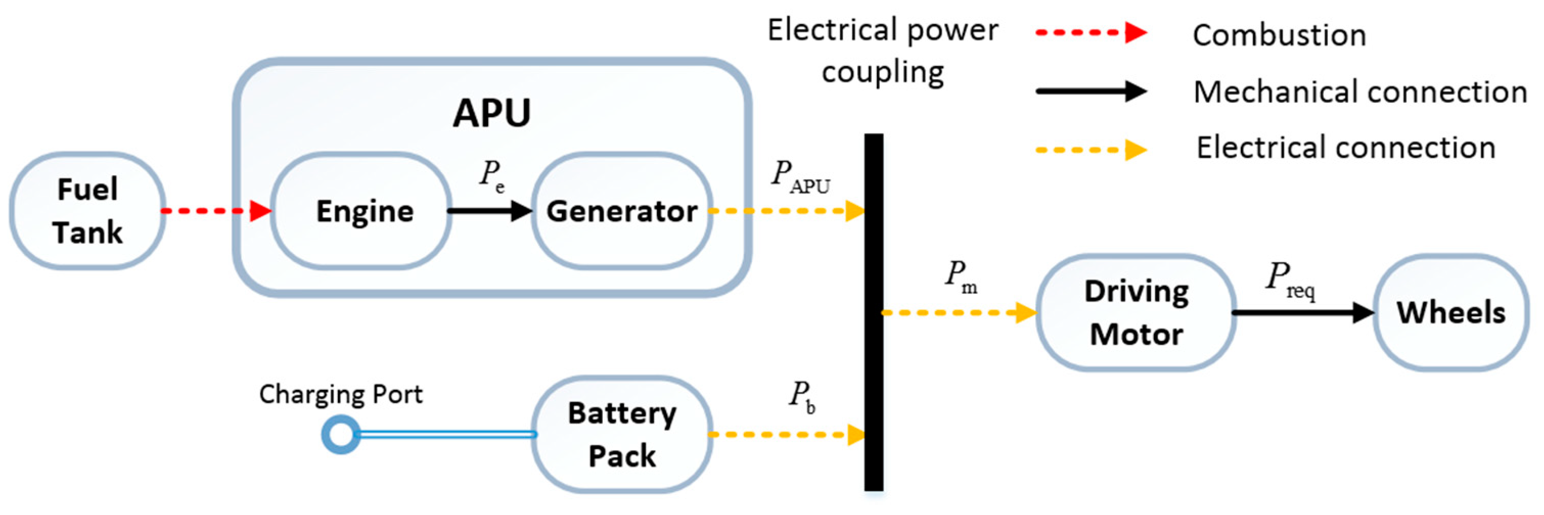
Environmental deterioration and the increasing shortage of petroleum resources have greatly increased the demand for energy-saving and environmental protective vehicles. The new energy vehicle technology is regarded as an excellent way to simultaneously address the energy crisis and insecurity and reduce environmental impacts [1]. As a type of plug-in hybrid electric vehicle (PHEV), extended-range electric buses (E-REBs) can coordinate the energy allocation between batteries and the auxiliary power unit, and prolong the mileage of pure electric vehicles while improving the fuel economy. Thus, extended-range electric buses have gained growing attention from vehicle manufacturers and customers [2,3].

Energy management is still a technical puzzle faced by hybrid electric vehicles because it not only aims at the minimum energy consumption, but also needs to take into consideration the vehicle dynamic performance, emission performance and the characteristic of each component. Due to the presence of multiple power sources, the reasonability of energy allocation directly affects the dynamic performance and fuel economy of vehicles [4]. However, the conventional energy management strategy only considers a single performance index and cannot achieve an overall optimization. Thus deeper research shows the energy management has gradually transited from the initially single goals of fuel depletion or emission to the currently multi-goal real-time intelligent integrated control. So far, the control strategies can be divided into rule-based and optimization-based energy allocation strategies [5].

In the first category, the vehicle working states are firstly divided according to pre-set control rules and then controlled separately. The rules are set to make the engine, generator and batteries work within the pre-set high-efficiency zones, but are only slightly dependent on specific working conditions and thereby operate in real-time. The two main directions of this category are the control strategies based on logic thresholds or fuzzy rules [6]. Firstly, the logic thresholds are usually the state of charge (SOC) of battery power or the speed signals of vehicles, which allow for switching between different operation modes [7]. Its disadvantage is that the dynamic performance of the vehicle will be greatly reduced when the work mode enters the charging-sustaining phase. The control strategies based on fuzzy rules control energy allocation via the use of fuzzy algorithms. Firstly, the control parameters are fuzzified into a power allocation factor, and thereby the driving system is controlled [8,9]. The common problem of rule-based strategies is that energy can only be allocated according to fixed rules without considering optimization, so the fuel consumption is relatively high.

The energy management of extended-range electric vehicles is essentially aimed to solve a multi-objective nonlinear optimization problem. Since the major objective is the minimization of systematic energy consumption, the energy control strategies based on global optimization and instantaneous optimization algorithms have been widely studied. As one global optimization algorithm, PMP constructs a Hamilton function, and when the Hamilton function reaches the minimum value under constraints, the target function is also minimized [10]. Dynamic programming (DP), another global algorithm, divides the whole working condition into several segments, and starting from the final state, reversely calculates the initial state and finally selects the controlling rule that makes the target function reach the minimum value as the optimal strategy [11,12]. However, both PMP and DP can get the optimal solution only when the whole driving cycles are known. Since the road conditions and driving behaviors are all unknown in real driving, global optimization algorithms are unfeasible in reality, but can be used as the benchmark for real-time energy management strategies. With the same hybrid electric vehicle model, Yuan compared DP and PMP and found their control effects were similar, but PMP was faster [13].

The energy management based on instantaneous optimization does not need any information about driving cycles and can be controlled in real-time according to the real driving conditions. The DP-developed stochastic dynamic programming (SDP) control strategies utilize DP algorithms to solve a number of working conditions, and apply the datasets as-obtained into neural network training [14]. In real applications, the real-time working conditions are substituted into the classifier to form energy distribution relations. Similarly, the artificial intelligent algorithms for energy management also include neural network control [15], particle swarm optimization [16], and genetic algorithm [17,18]. These Artificial Intelligence-strategies are faced with the problem of large amount of data training and too much computation in real-time operation. Model prediction control is aimed to model the controlled object, predict the output according to the vehicle state as-collected, optimize the predicted value, and input the resulting optimal energy allocation into the control system [19,20]. Borhan built an energy optimization control strategy based on model prediction and the simulations showed in the recycled working conditions of UDDS, the MPC control strategy reduced the oil consumption by 4.7% than the rule-based control strategy [21]. ECMS originating from PMP finds the minimum value through real-time solving the target function, and obtains the instantaneous energy distribution relation between batteries and APU [22]. However, the co-state of ECMS is constant and cannot well adapt to different working conditions in real tests. Thus, researchers have proposed adaptive-ECMS (A-ECMS) which is developed on the basis of ECMS. It can adjust the co-state value of Hamilton function in real time according to the operation state of the vehicle. The strategy can well adapt to the actual operation state and make the important vehicle performances reach the ideal value. Gu put forward an adaptive ECMS based on driving pattern recognition, and by identifying the information of working conditions, it adjusted the value of co-state to adapt to different working conditions [23]. Mahyar proposed to use GPS and ITS to predict the working conditions and built an A-ECMS control strategy based on reference SOC, so that the real SOC could decline along with the reference SOC curve [24]. According to the optimal co-state values under different driving conditions, Onori et al. plotted a co-state map and used SOC feedback to build a linear co-state function, which performed well in simulations [25,26]. Because A-ECMS has the characteristics of strong adaptability, good real-time performance and excellent control effect, it is selected as the energy management strategy of this paper.

1.2. Motivation

The objective of energy management strategy for an E-REB is to guarantee the dynamic performance of the E-REB during operation. Meanwhile the strategy ensures the SOC is always greater than the pre-set value and makes the final SOC close to the pre-set value, which not only protects the battery pack, but also fully uses the battery pack power.

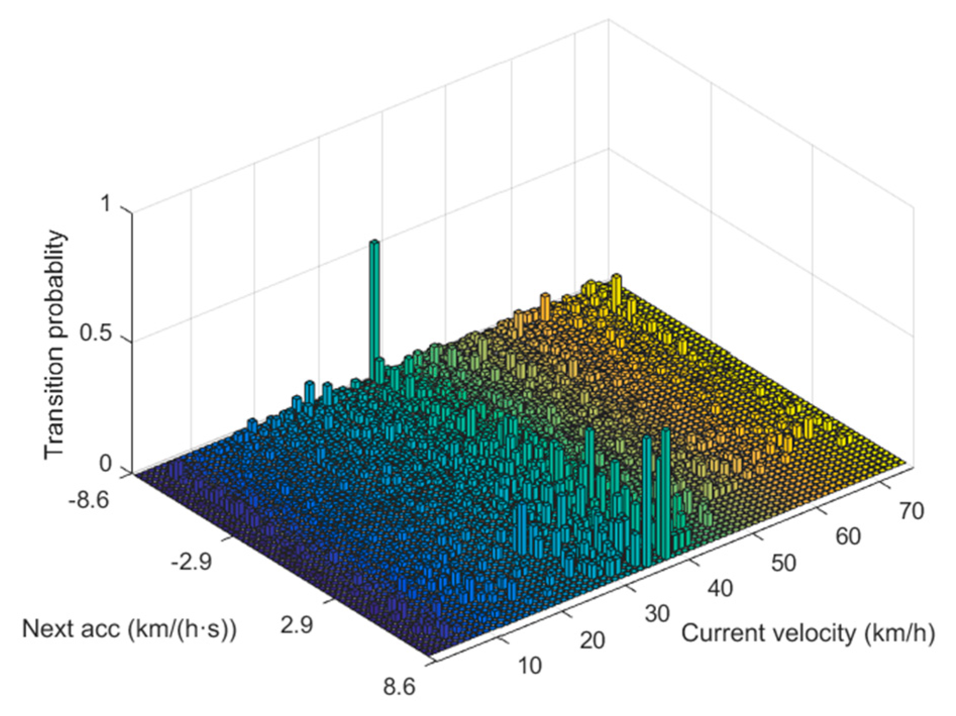
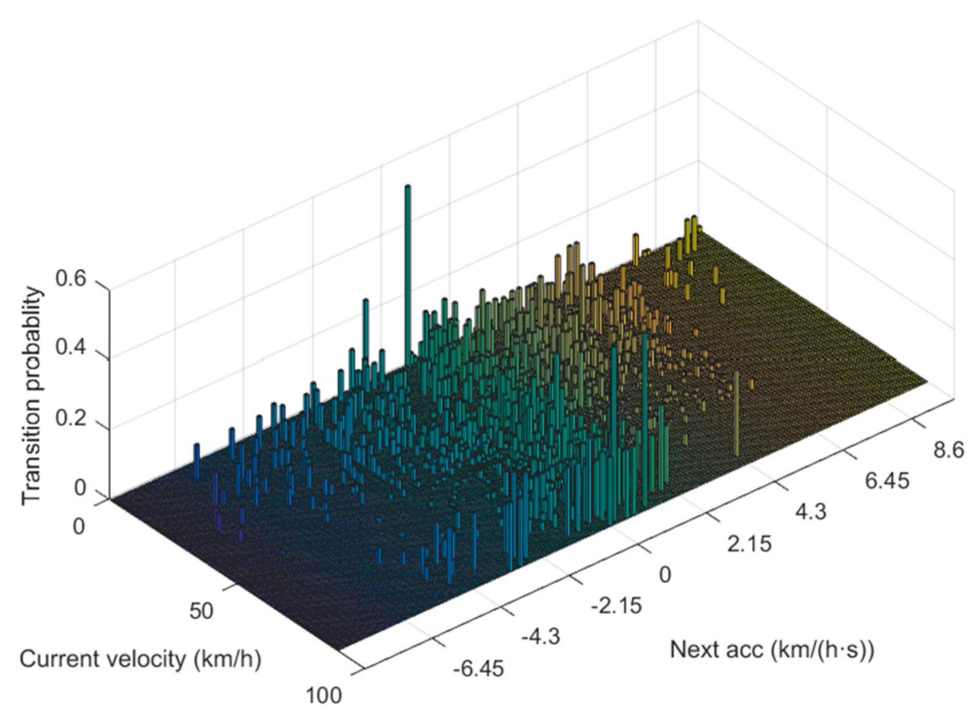
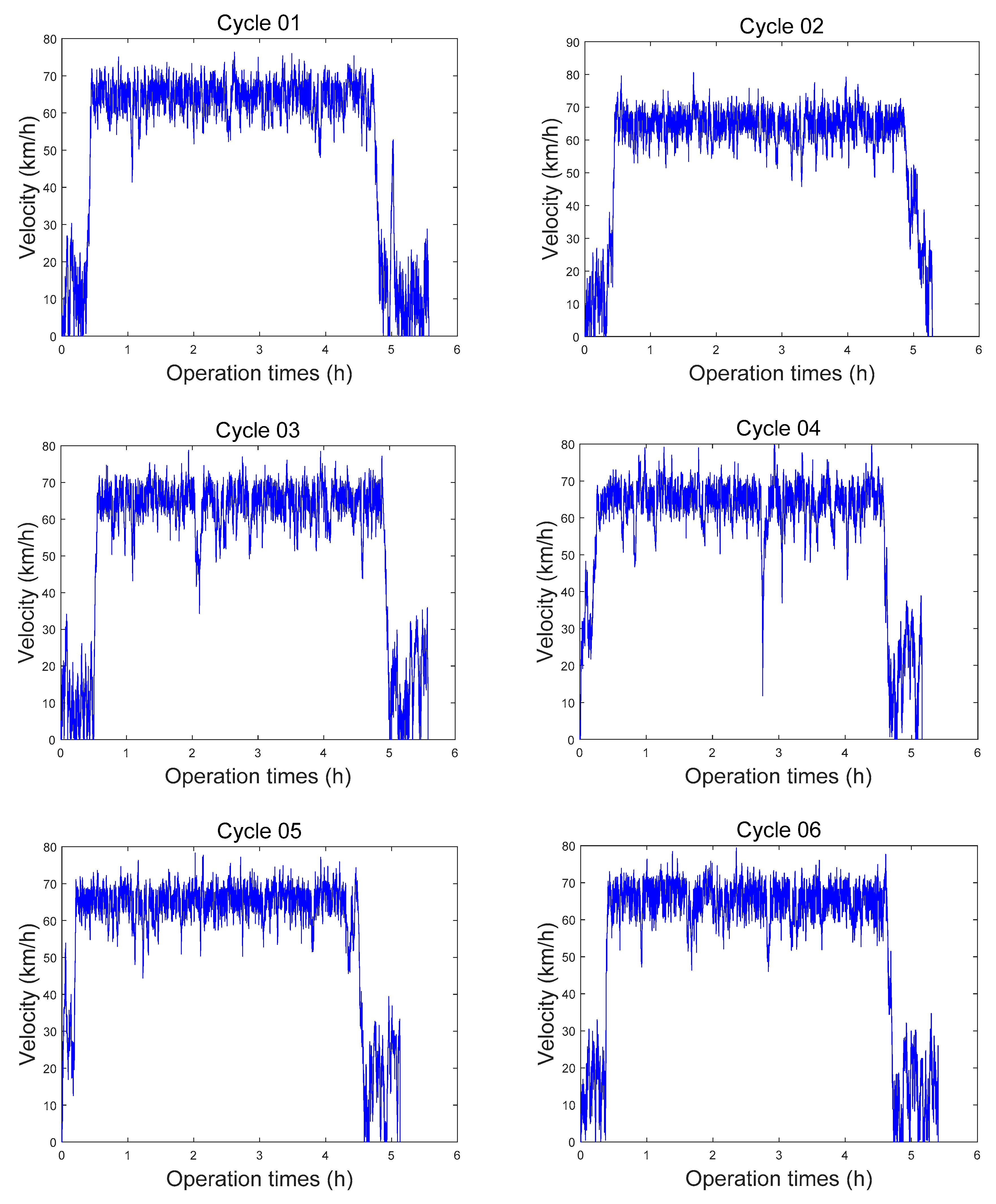
In order to meet the above performance requirements, the co-state value needs to be adjusted in real time according to the vehicle status. The motivation for this is explained as follows: (1) to solve the optimal co-state value, the Hamilton function and co-state equation for E-REB should be developed based on PMP; (2) the co-state is affected by driving distance and working conditions, so in order to establish the relationship between the co-state and its influencing factors, the target driving cycles are needed, however, there is often a lack of TDCs in practice. In order to solve this problem, the Markov chain based generation technology is proposed; (3) by the way of making the fuel consumption close to the optimal control result, and the final SOC value is similar to the pre-set value, SOC reference curve should be reasonably designed; (4) taking the SOC deviation value as the independent variable, the co-state adaptive function is established by PI control technology; (5) also, the initial value of SOC also has a significant impact on the co-state, thus the change of co-state function should be considered under different initial values.

1.3. Major Contribution

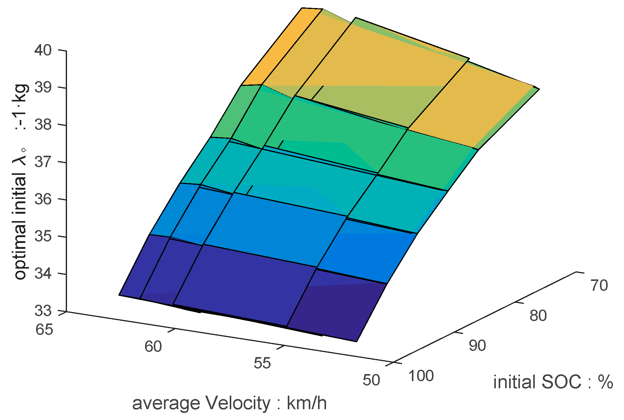
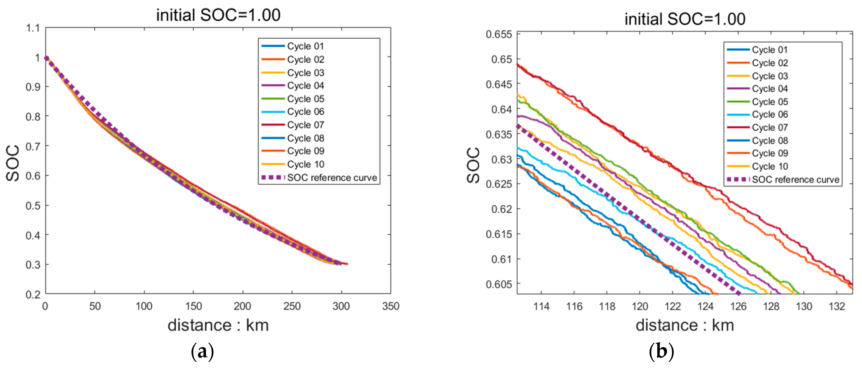
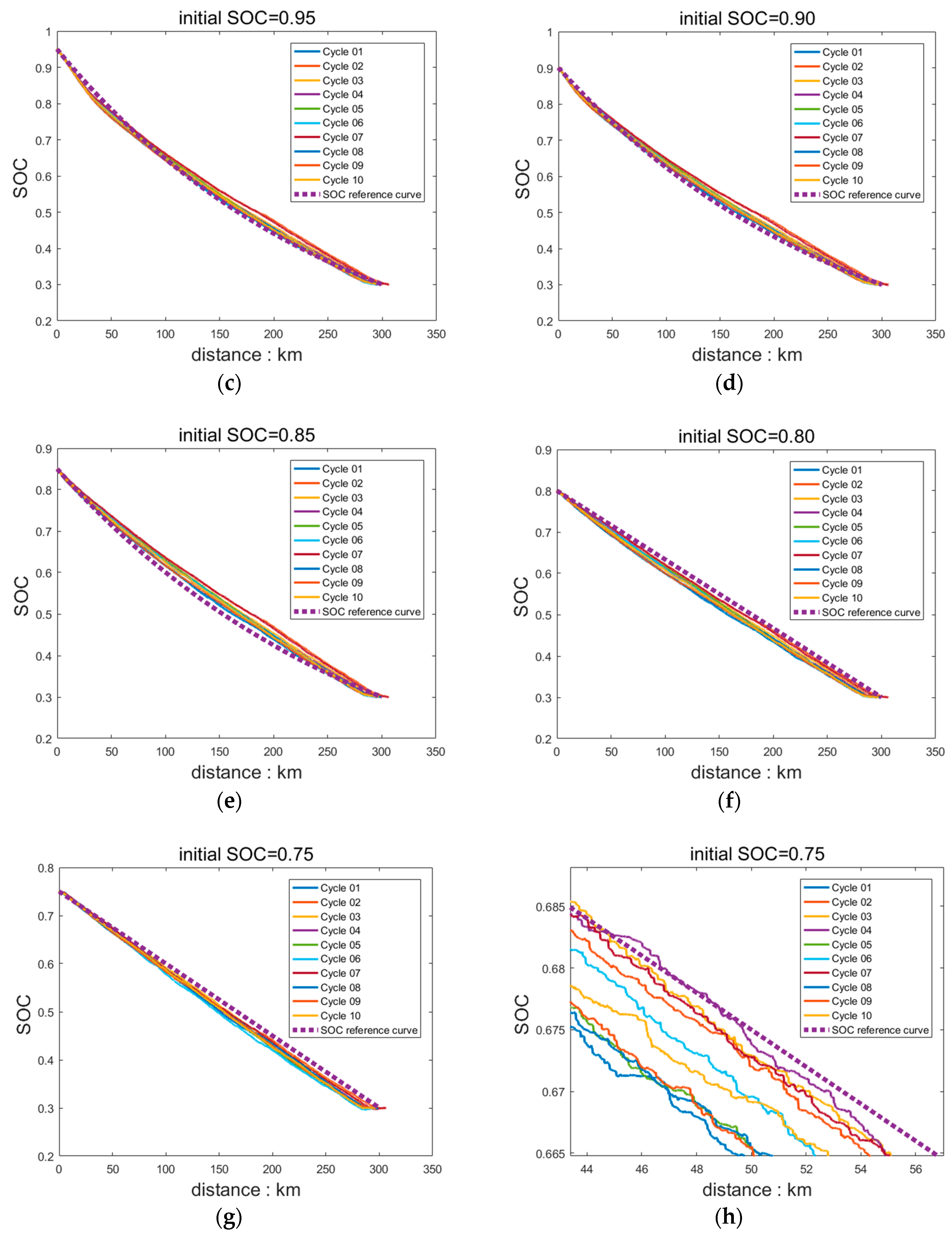
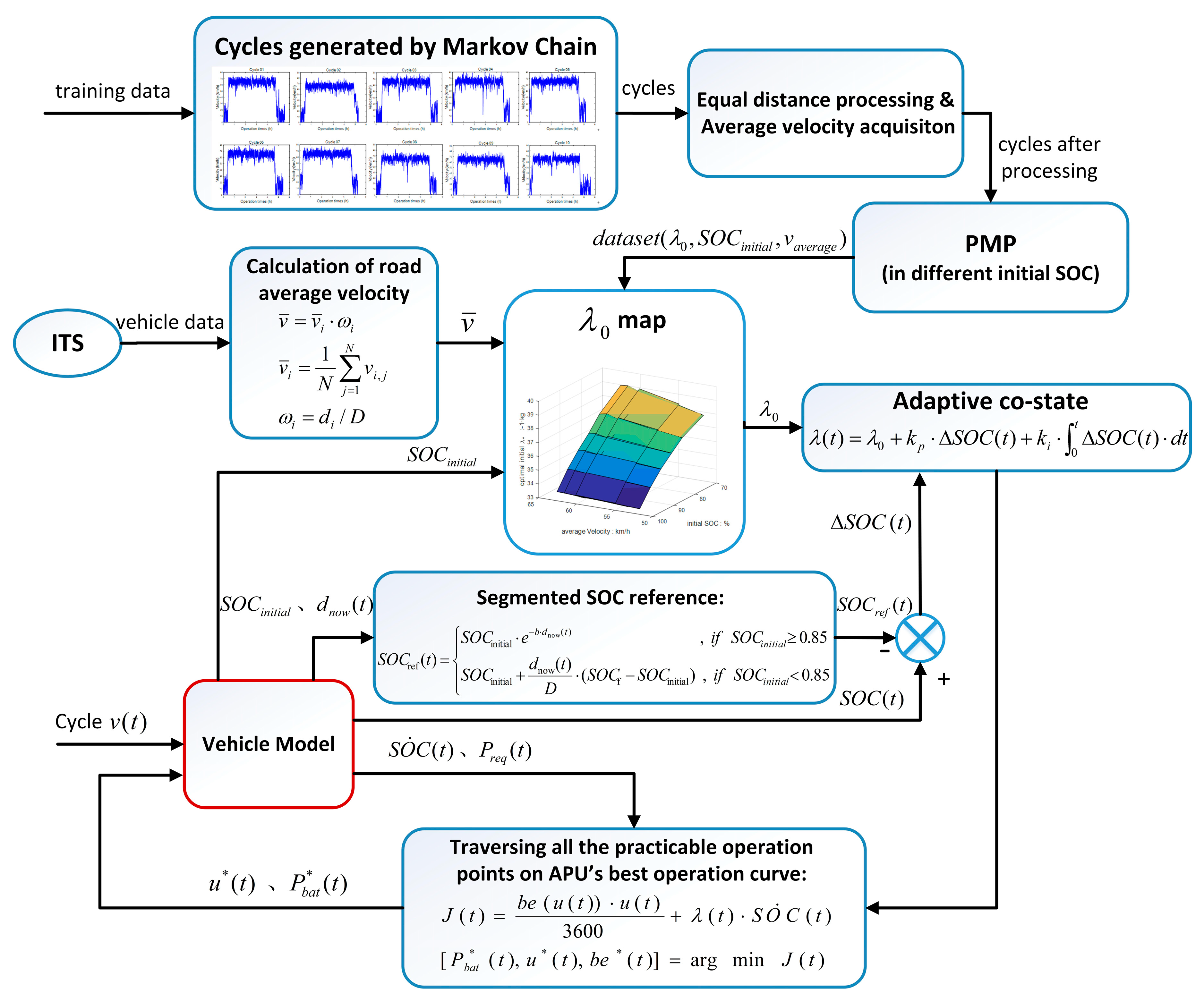
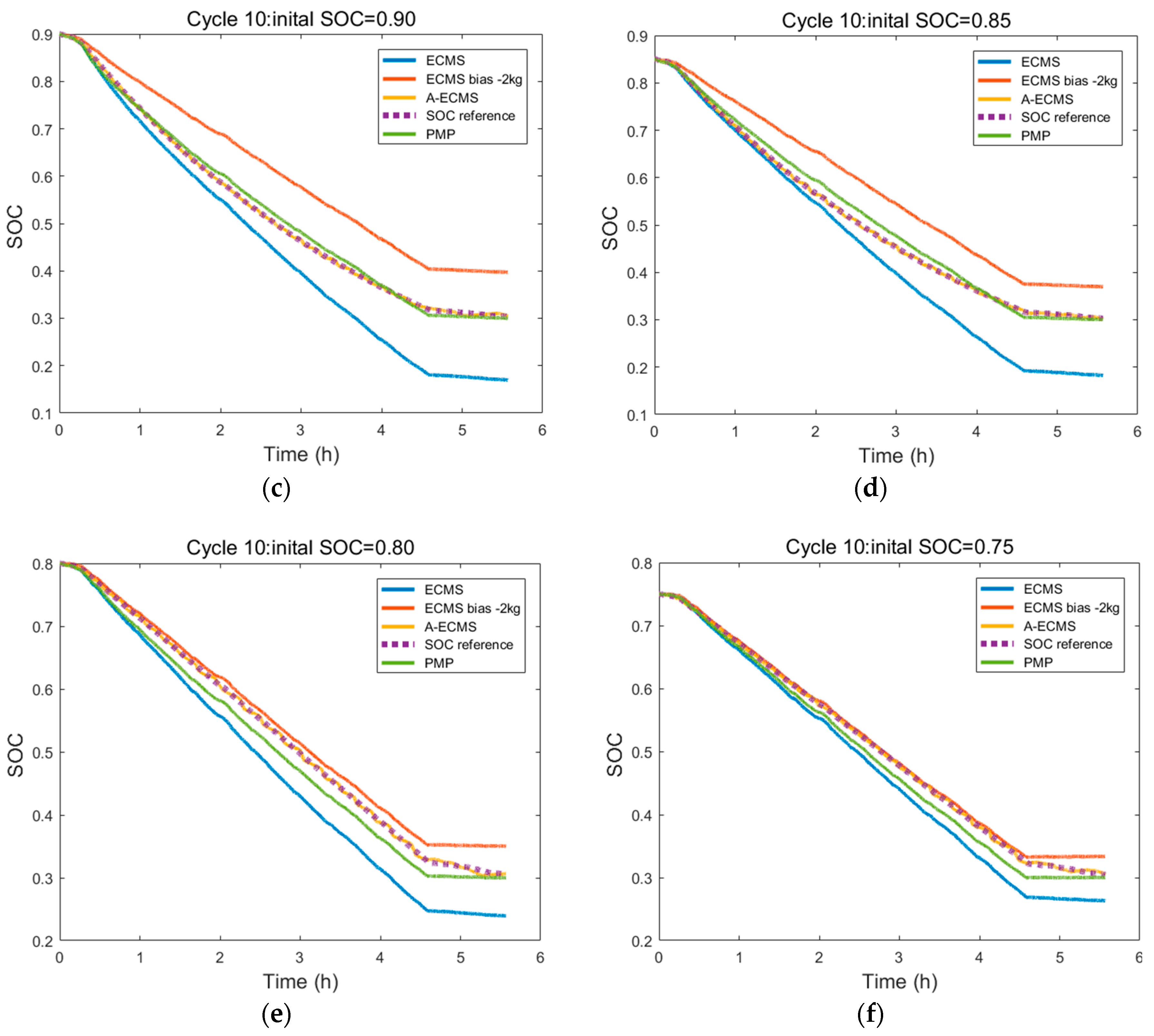
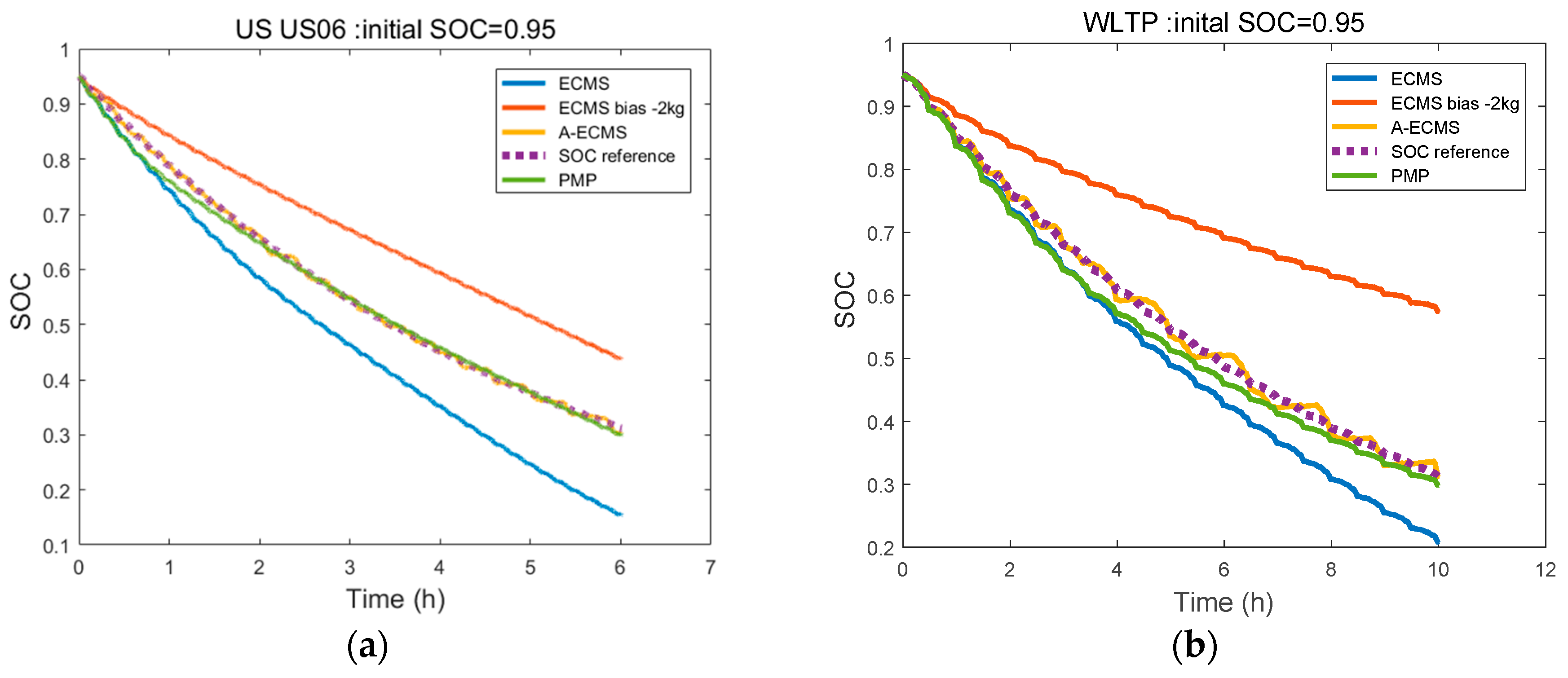
During formulation of A-ECMS, the key is to build a co-state adaptive function, which fully considers the effects of initial SOC, driving distance, and working conditions on the co-state. Since this study was targeted at extended-range electric buses operating on fixed routes, the driving distance could be ignored. The co-state function consisting of fixed term and dynamic term was designed. To determine the fixed term, we first had to get the optimal initial co-state map, which could be determined by solving multiple target driving cycles by using PMP. However, during control strategy research, there are always few working conditions suitable for the exploitation goal, which largely hinders the determination of concrete control strategy parameters and the simulation of control effect. For this problem, a goal condition generation method based on Markov chain was proposed. The working condition was gradually generated through the formation of a highway and city transition probability matrix. Furthermore, with the ITS-acquired vehicle information, the average vehicle speed was determined by weighted averaging. Together with the initial SOCs of vehicles, the fixed terms could be determined by interpolating the co-state map. The role of the dynamic term was to make the SOC at termination be equal to the set value, so as to make full use of the electrical energy. It usually can be realized by following the reference SOC. However, the common SOC reference curve is a linear function of SOC and distance, which totally disobeys the ideal solution. A segmented SOC reference curve was put forward according to the optimal SOC changing curves under different initial SOC conditions solved using PMP. When the initial SOC was large or small, an exponential reference curve and a linear reference curve were selected, respectively, which better fitted the variation of the optimal SOC. With the introduction of PI, the deviation of the real SOC from the reference curve was regarded as the input to real-time adjust the co-state dynamic term, so as to follow the reference curve. During the research, A-ECMS was simulated under different working conditions and different initial SOCs. Results showed A-ECMS could meet the design requirements and was well adaptive.

1.4. Outline

This study is organized as below: Section 2 introduced the mathematical model and concrete parameters of E-REB; In Section 3, the PMP algorithm targeting at E-REB is developed and thus the co-state differential equation is achieved. In Section 4, Markov chain was used to generate the target driving cycles; In Section 5, the co-state map and SOC reference curve were acquired, and A-ECMS was designed through PI control. In Section 6, the A-ECMS, ECMS and PMP were simulated and comparatively analyzed under different target driving cycles and different initial SOCs. Finally, the conclusions are summarized in Section 7.

2. E-REB Model Description

2.1. Powertrain and Parameters

The extended-range electric bus studied here is the inter-city passenger car travelling between Changchun and Shenyang, and its powertrain structure is showed in Figure 1. The E-REB is powered by an auxiliary power unit (APU) and a battery pack. The APU consists of the engine and the generator, while the engine drives the generator to generate power. The output power of the APU is coupled with that of batteries, and the electric power is converted by a driving generator to machinery power, and then the main reducer and the differential further transfer the energy to the wheels. The parameters of main vehicle components are listed in

Table 1. Main component parameters of E-REB.

Component	Parameter	Value
Engine	Max speed	4000 rpm
	Max power	95 kW
	Max torque	311 Nm @ 2200 rpm
Generator	Max speed	5000 rpm
	Rated power	95 kW
	Rated torque	420 Nm @ 0~2160 rpm
Battery pack	Type	Lithium-ion
	Capacity	300 Ah
	Rated voltage	576 V
Driving motor	Max speed	2000 rpm
	Peak /Rated power	180/120 kW
	Peak/Rated torque	1800/1200 Nm @ 0~955 rpm

.

2.2. Key Component Model

2.2.1. Battery Model

The battery pack consists of 156 battery cells in series, the total capacity of which is 300 Ah and the rated voltage is 576 V. Then ten battery cells in series are selected and tested at ambient temperature 25 °C. The data of charge/discharge resistance, open circuit voltage (OCV) and SOC from the ten cells are fitted in Figure 2.

The batteries are constructed using the internal resistance equivalent model (Rint model). At the discharge stage, the total power of the batteries P_bat is equal to the external power P_b and internal resistance R_int depletion. At this moment, the internal resistance is discharge resistance R_dc. At the charge stage, the external power P_b charges the batteries, where the internal resistance is charging resistance R_c. The open circuit voltage U_ocv and the internal resistance R_int are both correlated with SOC. It is supposed the batteries are maintained at 25 °C, or namely the effect of temperature on internal resistance is ignored:

$$P_{bat}=U_{ocv}(SOC)\cdot I=I^2\cdot R_{int}(SOC)+P_b$$

(1)

The current can be solved by Equation (1) as follows:

$$I=\frac{U_{oc}(SOC)-\sqrt{U_{oc}{(SOC)}^2-4P_b\cdot R_{int}(SOC)}}{2R_{int}(SOC)}$$

(2)

The changing rate of SOC can be expressed as follows:

$$S\dot{O}C=d(\frac{Q_b-{\displaystyle {\int }_0^{t}Idt}}{Q_b})/dt=-\frac{I}{Q_b}$$

(3)

where Q_b is the capacity of the battery pack.

2.2.2. Driving Motor Model

This extended-range electric bus is driven by a permanent magnet synchronous motor, and its efficiency map at the rated power is showed in Figure 3. The driving motor efficiency at given rotating speed and torque could be determined by the lookup-table interpolation method. When the driving motor works as a generator (braking energy recovery stage), the efficiency map is symmetrical. The efficiency of the driving motor is:

$${\eta }_m={\eta }_m(n_m,T_m)$$

(4)

The coupling total power P_m supplies to the driving motor, the motor output power is delivered by the transmission to the wheels, so as to meet the driving demanded power P_req, and its power transfer is expressed as:

$$P_{req}=P_m\cdot {\eta }_m\cdot {\eta }_T$$

(5)

where η_T is the transmission efficiency.

2.2.3. APU Model

As for an instantaneous energy management strategy, the optimal working point of each demanded power is computed offline in advance, which largely reduced the computational amount and favored the timeliness of the strategy. The optimal working point of APU is defined as to meet the demanded output power of APU and to minimize the fuel consumption. The optimal working points at different APU power values is connected, forming the optimal operation curve of APU. Since the output power and fuel consumption rate of APU are affected jointly by the engine and the generator, the characteristics of these two parts should be integrated to solve the optimal working curve. The output power of APU was expressed as:

$$P_{APU}=P_e\cdot {\eta }_g(n_g,T_g)=P_e\cdot {\eta }_g(n_e,T_e)$$

(6)

where η_g is the generator efficiency, n_e is the rotation speed and T_e is the torque. The fuel consumption rate of APU was calculated as:

$$be=be(n_e,T_e)$$

(7)

The universal characteristics and APU optimal operation curve of the engine are shown in Figure 4. Unlike the optimal working curve of the engine, that of the APU is integrated the generator efficiency. The minimum fuel consumption of each disperse power was plotted in Figure 5. Since the maximum output power of APU is 85 kW, the fuel consumption rate is very low when the output power of APU is 40–50 kW. Since the optimal working point of each discrete power is only and known, the rotating speed and torque of a working point can be determined if the allocation power of APU in the energy management algorithm is known.

2.3. Dynamic Model

According to the driving dynamic equation of a vehicle, the driving force can be expressed as:

$$F_t=mg\cdot f+\frac{C_{D}A{v}^2}{21.15}+\sigma m\frac{dv}{dt}$$

(8)

$$P_{req}=\frac{v}{3600}\cdot F_t$$

(9)

The symbols and their values are shown in

Table 2. E-REB model parameters.

Symbol	Parameter	Value
m	Vehicle mass	11,718 kg
f	Rolling resistance coefficient	0.01
CD	Air resistance coefficient	0.7
A	Windward area	8.6 m2
σ	Rotational inertia coefficient	1.1
$i_o$	Main ratio	4.875
r	Rolling Radius	0.511 m
ηT	Transmission efficiency	0.9

.

3. PMP Algorithm Formulation

Since PMP is the basis of ECMS, complete driving cycles are needed to solve the optimal control rate under the constraint conditions. The goal of the optimal energy management of a hybrid electric vehicle is that: the power of APU and the battery pack is allocated to minimize the fuel consumption while meeting the driver's required power P_req [27]. For extended-range vehicles, since the APU and transmission system are decoupled, the working points of APU can be randomly selected under the premise of meeting the constraint conditions. At the end of driving, SOC reached the set minimum value SOC_f so as to fully utilize electric energy and reduce oil consumption. During the whole driving process, SOC is maintained at the reasonable range [SOC_f,SOC_initial] so as to prolong the service life of batteries. Meanwhile, the output power of APU should never surpass the demanded power and thereby enter the mode of APU charging batteries, which avoided the secondary energy transfer and increased the energy use rate. Taken together, the target function and constraint conditions of energy management of E-REB can be expressed as:

$$\mathrm{Minimize}J(t)={\displaystyle {\int }_0^{t_f}{\dot{m}}_f(u(t))}\cdot dt={\displaystyle {\int }_0^{t_f}\frac{be(u(t))\cdot u(t)}{3600}}\cdot dt$$

(10)

$$subjecttoS\dot{O}C(t)=-\frac{I(t)}{Q_b}$$

(11)

$$SOC\left(t_0\right)=SO{C}_{initial},SOC\left(t_f\right)=SO{C}_f$$

(12)

$$SOC\left(t\right)\in [SO{C}_f,SO{C}_{initial}]$$

(13)

$$u(t)=P_{APU}(t)\in [P_{\min },P_{\max }]andu(t)\le P_{req}(t)$$

(14)

Here m_f is fuel consumption rate (g/s); u(t) is the APU allocation power, as the control variable, which varies within [0,85] kW according to Section 2.2.3. SOC is a state variable and its termination value is usually SOC_f = 30%. The energy management Hamilton function is:

$$H=\frac{be(u)\cdot u}{3600}+\lambda \cdot S\dot{O}C$$

(15)

where λ is the co-state, which is time-variant during the solving process of PMP and can be expressed as:

$$\dot{\lambda }=-\frac{\partial H}{\partial SOC}=-\lambda \cdot \frac{\partial S\dot{O}C}{\partial SOC}$$

(16)

Since the partial derivatives in this equation cannot be directly solved, it can be further transformed according to Equation (3):

$$-\frac{\partial S\dot{O}C}{\partial SOC}=\frac{1}{Q_b}\cdot \frac{\partial I}{\partial U_{oc}(SOC)}\cdot \frac{\partial U_{oc}(SOC)}{\partial SOC}$$

(17)

According to the characteristics of battery pack in Figure 2, when SOC_f = 30%, the charge/discharge resistance nearly does not change with voltage. Namely under the restrictions of SOC, the battery internal resistance can be regarded as constant:

$$\frac{\partial R_{int}}{\partial SOC}=\frac{\partial U_{oc}}{\partial SOC}\cdot \frac{\partial R_{int}}{\partial U_{oc}}\approx 0$$

(18)

On this basis, the partial derivative of Equation (2) over U_oc can be determined:

$$\frac{\partial I}{\partial U_{oc}(SOC)}=-\frac{I}{\sqrt{U_{oc}{(SOC)}^2-4\cdot P_b{R}_{int}}}$$

(19)

The partial derivative of voltage over SOC can be determined from the battery characteristics in Figure 2, marked as k(SOC). Taken together, the state equation of the co-state can be expressed as:

$$\dot{\lambda }=\frac{\lambda }{Q_b}\cdot \frac{\sqrt{U_{oc}{(SOC)}^2-4\cdot P_b{R}_{int}}-U_{oc}(SOC)}{2R_{int}\sqrt{U_{oc}{(SOC)}^2-4\cdot P_b{R}_{int}}}\cdot k(SOC)$$

(20)

After the state equations of SOC and λ are determined, the PMP algorithm can be solved using the Shooting method [28]. However, for PMP as a global optimization algorithm, all information about driving cycles should be acquired in advance, and thus, PMP cannot be directly applied in a real environment. The instantaneous optimization algorithms ECMS and A-ECMS based on PMP will be introduced in Section 5. The driving cycle generation method based on Markov chain will be introduced in Section 4. With the PMP algorithm, the optimal initial value of λ was solved, forming the optimal initial λ maps at different vehicle speeds and different initial SOCs.

4. Markov Chain Based Target Driving Cycles Generation

During research on control strategies, usually real driving cycles suitable for the development goal are insufficient. For instance, this study on the energy management strategies for the fixed route from Changchun to Shenyang required similar simulation conditions of several driving cycles. However, the shortage of driving cycles largely hindered the determination of concrete control strategy parameters and the simulation of control effect. To achieve this goal, we put forward a target driving cycle generation method based on Markov chain. The Markov chain method is widely used in speed prediction. Xie adopted it to forecast velocity sequences at every current state, with post-processing algorithms to moderate fluctuations of the prediction results like average filtering [29]. In addition to forecasting the vehicle speed, Liu forecasted the demand power accurately through a Markov chain approach. According to the current vehicle running state, the probability transfer matrix is used to estimate the demand power at the next time [30,31]. In fact, the speed prediction is intrinsically linked to the demand power prediction. According to the vehicle dynamics equation, the conversion of vehicle speed and demand power can be performed. The above methods all use Markov chain for short-term prediction. In contrast, this paper uses it to generate complete driving cycles. The main purpose is to perform optimal co-state calculations, reference curve solving and verification, rather than real-time forecasting. Based on the collected data and the data of typical driving cycles, a probability transition matrix is formed, and thereby the simulated driving cycles close to real data are generated.

During a Markov process, the future state and the past state of the system are mutually independent. The current state of the system is known, and the system state at any time is related with the current state, but not with the past state [32]. Then the vehicle speed ν_k+1 at step k+1 of discrete time is decided by the vehicle speed ν_k at step k of discrete time. Thus, the complete driving cycle can be generated stepwise starting from the initial status ν₁ = 0 km/h. The Markov status space consists of the discrete vehicle speed and acceleration; let the discrete vehicle speed be ν_i (i = 1,2,Λ,p), the discrete acceleration be a_j (i = 1,2,Λ,q), and the acceleration at step k+1 be a_k+1. Then starting from the current state ν_k = ν_i, the conversion probability reaching the next state a_k+1 = a_j can be expressed as:

$$p(a_{k+1}=a_j|v_k=v_i)=p_{ij}=\frac{N_{ij}}{{\displaystyle \sum _{j=1}^q{N}_{ij}}}$$

(21)

where p_ij is the transition probability from the current vehicle speed ν_i to the acceleration a_j of the next state; N_ij is the number of occurrences of the event where the current vehicle speed ν_i reaches the acceleration a_j of the next state; ${\displaystyle \sum _{j=1}^q{N}_{ij}}$ is the total number of event occurrences of the current vehicle speed ν_i reaching the acceleration of the any next state.

Then the target driving cycle from Changchun to Shenyang is analyzed. Using Google Map, the driving cycle from Changchun to Shenyang can be generally divided into three segments: (1) from city of Changchun to the highway junction: 5.4 km; (2) highway: 277 km; (3) from the highway junction to the city of Shenyang: 12.6 km. Of them, (1) and (3) correspond to city conditions, while (2) is a highway condition. Thus, the probability transition matrix should be divided into a city-matrix and a highway-matrix, to separately calculate the data statistics and matrix generation, respectively. The city road collected data, representing driving cycles such as FTP75 and ChinaCityBus are used to generate the city-matrix; for the highway collected data, representative driving cycles such as US_SC03 and Highway are used to generate the highway-matrix. The transition probability maps are shown in Figure 6 and Figure 7.

After the probability transition matrix is determined and under the known current vehicle speed, the acceleration at the next state is determined according to sampling by probability, and the vehicle speed at the next state is further determined:

$$v_{k+1}=v_k+ac{c}_{k+1}\cdot dt$$

(22)

Taken together, the driving cycles are generated segment-wise by using the Markov probability transition matrix. To simulate the variation of each driving distance during real driving, a random error δ ∈ [0,5%] is introduced. When each segment of driving cycle is generated, the effect of random error is considered. Based on the above conditions, in Figure 8, 10 simulated driving cycles (Cycle 01~10) are formed and used to determine the energy management strategy parameters and validate the control effect. The specific statistics of driving cycles and the solution results of PMP will be introduced in Section 5, and the solving process of PMP will be illustrated in Section 6.

5. Adaptive-ECMS

5.1. Co-State Map Generated for ECMS

ECMS is an extension of PMP and an instantaneous optimization algorithm that does not need the information of whole driving cycles. Based on Equation (15), ECMS continually finds the optimal solution at each single step k. The target functions at stage k can be expressed as:

$$J(k)=\frac{be(u(k))\cdot u(k)}{3600}+\lambda (k)\cdot S\dot{O}C(k)$$

(23)

In the basic ECMS, the value of co-state is equivalent to the optimal initial value λ₀ of the co-state, and thus, this strategy is also called Constant-ECMS (C-ECMS). λ₀ is mainly affected by the driving distance, the initial value of SOC, and the working conditions [33]. In this study, since the driving route is fixed, the effect of driving distance can be ignored.

The 10 as-generated driving cycles are used in PMP training; let the initial value of SOC be SOC_initial, and the average vehicle speed ν_average is used to characterize the working condition. The maps of λ₀ with SOC_initial and ν_average are plotted. During the generation of driving cycles, the error δ of each driving distance is considered, which would affect the accuracy of the map. Thus, the smallest distance d_min of the 10 driving cycles is selected for equidistance processing; the data when the driving distance is d_min under all driving cycles are used into PMP training. The information of PMP training under the 10 driving cycles after equidistance are summarized in

Table 3. λ₀ solving results by using the equal distance process.

Number	νaverage (km/h)	SOCinitial
		1.00	0.95	0.90	0.85	0.80	0.75
Cycle09	51.6853	−33.399	−34.5494	−35.4932	−36.2315	−36.9346	−37.7542
Cycle08	51.9578	−33.407	−34.5503	−35.4777	−36.229	−36.9626	−37.8124
Cycle01	53.2634	−33.413	−34.5773	−35.5221	−36.2579	−36.9967	−37.8462
Cycle03	54.8937	−33.522	−34.7074	−35.6664	−36.4219	−37.2319	−38.2886
Cycle10	55.0385	−33.496	−34.6745	−35.6334	−36.3932	−37.1821	−38.2179
Cycle05	58.8617	−33.530	−34.7165	−35.689	−36.429	−37.2883	−38.4523
Cycle04	59.6607	−33.559	−34.7494	−35.7163	−36.4997	−37.339	−38.4693
Cycle02	60.1133	−33.639	−34.8513	−35.8389	−36.6909	−37.6289	−38.9175
Cycle06	61.6337	−33.654	−34.9023	−35.9111	−36.7447	−37.7832	−39.0079
Cycle07	62.5894	−33.663	−34.888	−35.867	−36.6936	−37.6759	−38.949

. The table is converted to 3D maps (Figure 9) for ECMS interpolation to determine λ₀. Due to the limitation of training driving cycles, the average vehicle speed coverage is very narrow, so λ₀ in the parts beyond the range is solved through outward interpolation.

5.2. A-ECMS and SOC Reference Curve

Under the whole driving cycle, λ is constant and invariable during the solving process of C-ECMS, but λ is continually updated according to Equation (20) during PMP training. This means SOC_kmax ≠ SOC_f = 0.3 may occur at the end of the cycle. When SOC_kmax > SOC_f, λ is small and the electricity is not completely used, leading to excessive fuel consumption; when SOC_kmax < SOC_f, λ is large and the electricity is excessively used, which affects the service life of batteries. Thus, Adaptive-ECMS (A-ECMS) has been widely studied, so as to make SOC_kmax at the end of working conditions close to the preset value. As for A-ECMS, the co-state λ is varying during the operation, and the adaptive λ as-designed can be expressed as:

$$\{\begin{array}{l}\lambda (t)={\lambda }_0+k_p\cdot \Delta SOC(t)+k_i\cdot {\displaystyle {\int }_0^t\Delta SOC(t)}\cdot dt\\ \Delta SOC(t)=SOC(t)-SO{C}_{ref}(t)\end{array}$$

(24)

where k_p and k_i are the adjustment coefficients of the proportion step and the integral step, and SOC_ref is the SOC reference curve. By following the reference curve, the SOC_kmax at the end of driving cycle is close to the preset value SOC_f During the operation, the SOC is higher than the reference curve, indicating the electricity use is little and λ should be enlarged, so that the energy management strategy is leaning to electricity use; and vice versa.

The commonly-used SOC reference curve is SOC-distance linear curve [34]. However, in real situations, the SOC-distance is not completely linear, and thus this reference curve is blind to some extent. A segmented SOC reference curve is designed according to the changing curves under different initial SOCs of 10 cycles solved using PMP:

$$SO{C}_{\mathrm{ref}}(t)=\{\begin{array}{l}SO{C}_{\mathrm{initial}}\cdot e^{-b\cdot d_{\mathrm{now}}(t)}\hspace{1em}\hspace{1em}\hspace{1em}\hspace{1em}\hspace{1em}\hspace{1em}\hspace{1em},ifSO{C}_{initial}\ge 0.85\\ SO{C}_{\mathrm{initial}}+\frac{d_{\mathrm{now}}(t)}{D}\cdot (SO{C}_{\mathrm{f}}-SO{C}_{\mathrm{initial}}),ifSO{C}_{initial}<0.85\end{array}$$

(25)

$$b=\frac{1}{D}(\ln (SO{C}_{\mathrm{initial}})-\ln (SO{C}_{\mathrm{f}}))$$

(26)

$$d_{\mathrm{now}}(t)={\displaystyle {\int }_0^{t}v(t)dt}$$

(27)

where D is the total driving distance (km), and d_now(t) is the driven distance (km).

With different initial SOCs, the optimal changing curves of the 10 driving cycles and the SOC reference curves are determined (Figure 10). It should be noted during each solving process, the 10 whole driving cycles are used, rather than the cycles after equalizing them. The SOC changing curve of the optimal solution is arc-shaped (Figure 10). When SOC is large, λ is large, and the energy management strategy is leaning to electricity use, so the declining slope of SOC is very large. As the driving distance increased, λ was updated according to Equation (20) and thus declined, so the energy management strategy is leaning to oil use, and thus the declining slope of SOC gradually decrease. Moreover, as the initial value of SOC decreased, the radian of SOC changing curve declined and when SOC_initial is <0.85, it is close to a line. This is because the whole vehicle does not have enough electricity, leading to the relatively small initial value λ₀ of optimal co-state from the solving process. The strategy is leaning to oil use compared to the case of large initial SOC, so the declining slope of SOC at the early stage is small. Taking the above simulated data and the analysis together, for A-ECMS with initial SOC ≥0.85 or <0.85, an exponential reference curve or a linear reference curve are used, respectively. Together with Figure 10, it is clear that the segmented reference curve of SOC has very good fitting results.

5.3. Average Velocity Obtained from Traffic Information

The adaptive co-state function (24) can be divided into a dynamic term and a constant term. Specifically, the PI-adjusted part is the dynamic term and is variable during the driving process; while the constant term λ₀ can be determined from the interpolation of the map. Thus, the SOC_initial and average vehicle speed ν_average are needed to determine λ₀. In particular, the initial SOC can be determined from the battery management system. The average vehicle speed can be determined by statistically analyzing the information of the driving vehicle, with the use of ITS.

The route from Changchun to Shenyang is already divided as mentioned above. The three sections from Changchun city to the highway junction, highway, and from the highway junction to Shenyang city are marked as 1, 2 and 3, respectively. The distances of three sections are marked as d₁, d₂ and d₃ with the total distance of D. To calculate the average vehicle speed ${\overline{\nu }}_i\in \left\{1,2,3\right\}$ of section i, we have to calculate the average of ITS-acquired vehicle data of section i:

$${\overline{v}}_i=\frac{1}{N}{\displaystyle \sum _{j=1}^N{v}_{i,j}}$$

(28)

where N is the number of vehicles in section i, and ν_i,j is the vehicle speed of vehicle j in section i. It should be noted since most of the vehicles recorded by the ITS are passenger vehicles and their speeds may surpass that of the extended-range bus, the data disobeying the driving requirements of the bus should be excluded. Furthermore, the average vehicle speed at each section is weight-averaged to get the total average vehicle speed:

$$\overline{v}={\displaystyle \sum _{i=1}^3{\overline{v}}_i\cdot {\omega }_i}$$

(29)

$$\{\begin{array}{l}{\omega }_i=\frac{d_i}{D}\\ {\omega }_1+{\omega }_2+{\omega }_3=1\end{array}$$

(30)

where ω_i is the weight of section i, which reflects the effect of section distance on the total average vehicle speed. Since the highway section is the longest, the total average vehicle speed is also very large.

5.4. Architecture of A-ECMS

As a summary of the above flowchart, the architecture of A-ECMS is shown in Figure 11. Firstly, data of representative driving cycles and collected data are used to generate a city-highway probability transition matrix, and with Markov chain, the target driving cycles are formed. The equidistance driving cycles are solved by PMP, forming the optimal co-state initial values under each driving cycles with different initial SOC, forming a map. In real-time operation, the ITS data are weight-averaged, and together with the initial SOCs provided by the BMS system, λ₀ is determined from interpolation. A vehicle provides information of real-time driving distance, demanded power, SOC and its changing rate. With the segmented SOC reference curve established from real-time follow-up as the goal, the adaptive λ is adjusted through PI control. Within the range of constraint conditions, the optimal working curve of APU is traversed so as to solve the minimum value of the target function J. Finally, the optimal APU and the battery allocation power are determined, and substituted into the whole-vehicle model for control.

6. Validation and Discussion

6.1. Optimal Initial Value of Co-State Solved by PMP

With PMP, for the 10 driving cycles as-generated, the optimal initial values of co-state are solved under different initial SOCs. With the solutions of equidistance driving cycles (Table 3), the map of λ₀ is plotted. In this Section, the complete information of driving cycles are utilized to compare PMP, C-ECMS and A-ECMS. The initial co-state to be substituted into PMP is gradually adjusted via the Shooting method until the difference between the final SOC and the preset value after the PMP meets the required precision. The initial co-state from the final searching is selected as the optimal initial value. With Cycle 10 for instance, the optimal initial co-state is solved at the initial SOC of 1.0, 0.95, 0.9, 0.85, 0.8 and 0.75 (Figure 12).

The initial value for the first searching can be selected empirically, and the value selected closer to the real value would make the searching faster. In this study, when the initial SOC is 1.0 or 0.95, the initial value of the first searching is −33 kg; under other conditions, it is −36 kg. Similarly, the optimal initial co-state under different initial values of SOC for the 10 driving cycles is solved (

Table 4. λ₀ solving results and statistical data of 10 cycles.

Number	vaverage (km/h)	d1 (km)	d2 (km)	d3 (km)	D (km)	SOCinitial
						1.00	0.95	0.90	0.85	0.80	0.75
Cycle01	53.1239	5.540	276.721	13.210	295.471	−33.413	−34.5654	−35.5105	−36.2576	−36.9958	−37.8421
Cycle02	58.0003	5.531	287.352	13.150	306.034	−33.753	−34.973	−35.9698	−36.7981	−37.7928	−39.0112
Cycle03	53.7017	5.563	281.166	12.795	299.532	−33.5429	−34.7343	−35.6942	−36.4505	−37.2635	−38.3308
Cycle04	58.0786	5.537	281.048	12.867	299.456	−33.5874	−34.7864	−35.7439	−36.5218	−37.3703	−38.4551
Cycle05	58.0706	5.450	279.188	13.127	297.769	−33.5535	−34.7432	−35.7084	−36.4677	−37.3386	−38.4484
Cycle06	54.8340	5.566	277.619	13.020	296.210	−33.6573	−34.9013	−35.9199	−36.7521	−37.7667	−38.9854
Cycle07	58.3364	5.412	288.078	12.670	306.162	−33.7263	−34.9399	−35.9043	−36.7436	−37.7174	−38.8759
Cycle08	55.0633	5.532	280.125	13.103	298.761	−33.4223	−34.5745	−35.494	−36.2516	−36.9761	−37.7948
Cycle09	56.6853	5.633	276.396	13.125	295.153	−33.3999	−34.5601	−35.4928	−36.2384	−36.9499	−37.7511
Cycle10	53.3712	5.449	278.652	13.024	297.129	−33.5077	−34.6928	−35.648	−36.4061	−37.1943	−38.2107

). During the PMP solving process, the co-state continuously varied according to the updating Equation (20). When the different initial SOCs under the 10 driving cycles are outputted, the co-state changing curve under the optimal initial co-state is selected (Figure 13). Clearly, the co-state gradually declined with time. The changing range of co-state in (a) is about −3.5 kg, but is −1.5 kg in (f), indicating with a smaller initial SOC, the changing amplitude of co-state decreases. At the initial stage of (a), the changing rate of co-state is very large, but at the distance of 40–50 km, an evident turning point appeared and the changing rate of co-state decreased. This is because the electricity consumption led to the platform stage of SOC, as shown in the 20%–80% stage of SOC in Figure 2. At this moment, the changing degree of voltage U_oc with SOC is smaller, or namely the k(SOC) of updating equation and thereby the changing rate decreased.

As the initial SOC decreased, the turning point moved forward, which is because the insufficiency of initial electricity led to the earlier entrance to the SOC platform stage. There is no turning point in (e) or (f), which is because SOC at the initial stage of the operation has already entered the platform stage.

6.2. Comparison of Different Energy Management Strategies

In this study, the global optimization algorithm PMP, and its derivative instantaneous algorithms C-ECMS and A-ECMS are introduced. In this section, the three energy management strategies under different initial SOCs and the 10 generated driving cycles are compared. As shown in Section 6.1, during the solving process of PMP, when the initial SOC is 1.00, the changing range of co-state is about −3.5 kg; when the initial SOC decreases, the changing range of co-state becomes narrower; when the initial SOC is 0.75, the changing range is about −1.5 kg. In C-ECMS, the co-state is always the initial value. To illustrate the effect of the initial value of co-state on the effect of C-ECMS, we select two initial values with the bias of −2 kg. In the adaptive co-state function, the proportionality factor k_p is 0.2, and the integral coefficient k_i is 0.004. For Cycle 10 for instance, the simulation map is shown in Figure 14.

Clearly, the adjustment by PI makes the variation of SOC follow the SOC reference curve well, and at the end of driving, the final SOC is very close to the pre-set value (0.3). The SOC changing curves of A-ECMS and PMP are overlapped well, indicating the instantaneous optimization result is very close to the global optimized result. When the initial SOC is <0.85, the degree of overlap decreases slightly. This is because the reference curve of SOC is switched from an exponential function, when the initial SOC is large, to a linear function, when the initial SOC is low. The middle stage of the linear reference curves in Figure 10f,g are leaning to oil use, leading to the deviation of the SOC curves of A-ECMS and PMP at the middle stage in Figure 14e,f. Generally, however, when the initial SOC is low, the linear reference curve of SOC is closer to the SOC curve of PMP, which better ensures the lower oil consumption. Neither of the two types of C-ECMS meets the condition of making the final SOC close to the pre-set value. The co-state of unbiased C-ECMS is excessively large, leading to excessive discharge from the batteries; the co-state of the C-ECMS with bias of −2 kg is too small, so the electricity of batteries is not fully used.

The comparison of SOC changing curves of four energy management strategies show though the bias of two types of C-ECMS is constantly −2 kg, the difference between the SOC changing curves vary under different initial SOCs. Specifically, at very large initial SOC, the SOC changing curves of these two types of C-ECMS are largely different; at very small initial SOC, the differences decreases. It is indicated at very low initial SOC, the co-state determined from map interpolation is very small, which largely limits the changing rate of SOC. At this moment, with further decrease of the initial co-state, the effect of SOC on the whole driving cycle decreases.

In addition, the effectiveness of the system is verified by the standard driving cycles WLTP and US_US06. Due to the short simulation distance of these cycles, it is necessary to extend the distance to the same distance as the target driving cycles (290–300 km). The simulation results are shown in Figure 15. In the standard cycles, the A-ECMS can still make the final SOC converge to the pre-set SOC, and ensure the electric energy is fully utilized and the solution of oil consumption is close to that of PMP. In the US_US06 cycle, the results of A-ECMS and PMP are different in the first stage of operation (<1.5 h), but the results of the latter stage are very close. However, in the operation of the WLTP cycle, the SOC of A-ECMS is always greater than the SOC of PMP. This is because the difference between the standard driving cycle WLTP and the target driving cycle of the paper is too large, so that the SOC reference curve cannot be well adapted to this cycle. This shows that the A-ECMS can make the final SOC reach the expected value in different driving cycles. As long as the reference curve is adjusted according to the cycles, the result of the oil consumption solution can be close to the global optimization result.

The simulation results of Cycles 01~10 are statistically analyzed (

Table 5. Comparison statistics with initial SOC = 1.00.

Number	Final SOC				Fuel Consumption (kg)
	C-ECMS	C-ECMS(-2)	A-ECMS	PMP	C-ECMS	C-ECMS(-2)	A-ECMS	PMP
Cycle 01	0.1141	0.4121	0.2999	0.3004	17.9110	28.2983	25.5074	24.3694
Cycle 02	0.0788	0.3700	0.2975	0.3009	19.2109	29.2575	27.9867	26.8491
Cycle 03	0.1004	0.3957	0.2906	0.3008	18.2269	28.4817	26.5841	25.1481
Cycle 04	0.0969	0.3907	0.3019	0.3007	18.4140	28.6073	26.8725	25.4510
Cycle 05	0.1171	0.4060	0.3069	0.3004	18.8644	28.9469	25.9820	25.2288
Cycle 06	0.1128	0.3862	0.3022	0.2996	18.9374	28.458	27.1953	25.4218
Cycle 07	0.1047	0.3854	0.2963	0.3004	19.8999	29.6612	27.8810	26.6793
Cycle 08	0.1293	0.4268	0.3042	0.3000	18.1772	28.5881	25.6125	24.1148
Cycle 09	0.1273	0.4261	0.3044	0.3002	17.6741	28.1196	25.0490	23.6817
Cycle 10	0.1065	0.4010	0.3064	0.3006	17.9894	28.2285	26.1526	24.7016

,

Table 6. Comparison statistics with initial SOC = 0.95.

Number	Final SOC				Fuel Consumption (kg)
	C-ECMS	C-ECMS(-2)	A-ECMS	PMP	C-ECMS	C-ECMS(-2)	A-ECMS	PMP
Cycle 01	0.1211	0.4076	0.3035	0.2997	20.0642	30.0979	27.3669	26.2766
Cycle 02	0.0843	0.3643	0.2965	0.3007	21.3064	31.0145	30.3512	28.7851
Cycle 03	0.1064	0.3911	0.2919	0.3003	20.3453	30.2729	28.0594	27.0690
Cycle 04	0.1046	0.3859	0.2994	0.3008	20.5835	30.3917	28.7220	27.3925
Cycle 05	0.1262	0.4023	0.3022	0.3003	21.0894	30.7718	27.9162	27.1597
Cycle 06	0.1208	0.3795	0.3025	0.2993	21.1224	30.1799	28.7759	27.3507
Cycle 07	0.1121	0.3795	0.2962	0.3002	22.0665	31.4124	29.4395	28.6175
Cycle 08	0.1400	0.4210	0.3050	0.3008	20.4566	30.3412	27.4689	26.0750
Cycle 09	0.1408	0.4217	0.2988	0.3008	20.0433	29.9250	26.9613	25.6372
Cycle 10	0.1150	0.3966	0.3030	0.3005	20.1883	30.0272	28.1068	26.6365

,

Table 7. Comparison statistics with initial SOC = 0.90.

Number	Final SOC				Fuel Consumption (kg)
	C-ECMS	C-ECMS(-2)	A-ECMS	PMP	C-ECMS	C-ECMS(-2)	A-ECMS	PMP
Cycle 01	0.1750	0.4099	0.3068	0.2996	23.7514	32.1257	29.5778	28.1679
Cycle 02	0.1379	0.3663	0.2968	0.3007	24.9463	33.0341	31.8291	30.6878
Cycle 03	0.1597	0.3939	0.2985	0.3001	23.9973	32.3222	30.4358	28.9580
Cycle 04	0.1575	0.3869	0.2984	0.3000	24.2220	32.3742	30.3386	29.2607
Cycle 05	0.1876	0.3992	0.3038	0.3001	25.0373	32.6126	30.1988	29.0491
Cycle 06	0.1734	0.3763	0.3020	0.3001	24.7708	32.0144	30.7227	29.2799
Cycle 07	0.1675	0.3782	0.2854	0.2994	25.8026	33.3165	30.9027	30.4900
Cycle 08	0.2006	0.4224	0.2998	0.3002	24.3828	32.3437	29.2079	27.9447
Cycle 09	0.2008	0.4232	0.3076	0.3001	23.9537	31.9299	28.2447	27.4992
Cycle 10	0.1696	0.3970	0.3046	0.3000	23.8905	31.9899	29.4823	28.5116

,

Table 8. Comparison statistics with initial SOC = 0.85.

Number	Final SOC				Fuel Consumption (kg)
	C-ECMS	C-ECMS(-2)	A-ECMS	PMP	C-ECMS	C-ECMS(-2)	A-ECMS	PMP
Cycle 01	0.1910	0.3837	0.3024	0.2996	26.1578	33.0950	31.179	30.0414
Cycle 02	0.1532	0.3379	0.2921	0.3003	27.3240	33.9269	33.0170	32.5639
Cycle 03	0.1754	0.3673	0.2957	0.2998	26.3919	33.2790	31.5416	30.8269
Cycle 04	0.1734	0.3589	0.3017	0.2998	26.6208	33.2789	32.3868	31.1340
Cycle 05	0.1979	0.3666	0.3048	0.3004	27.2541	33.3523	32.0638	30.9375
Cycle 06	0.1844	0.3466	0.3043	0.3000	27.0162	32.8624	32.5282	31.1648
Cycle 07	0.1792	0.3478	0.2880	0.3000	28.0668	34.1402	33.2943	32.4012
Cycle 08	0.2144	0.3931	0.2987	0.3000	26.7266	33.2017	30.5049	29.8154
Cycle 09	0.2173	0.3945	0.3049	0.3005	26.3865	32.8099	30.3681	29.3865
Cycle 10	0.1825	0.3697	0.3009	0.3004	26.1897	32.9222	31.5386	30.4019

,

Table 9. Comparison statistics with initial SOC = 0.80.

Number	Final SOC				Fuel Consumption (kg)
	C-ECMS	C-ECMS(-2)	A-ECMS	PMP	C-ECMS	C-ECMS(-2)	A-ECMS	PMP
Cycle 01	0.2481	0.3638	0.3029	0.3000	30.0416	34.3067	32.9472	31.9411
Cycle 02	0.2046	0.3175	0.2947	0.3001	30.9870	35.1225	35.9526	34.4765
Cycle 03	0.2320	0.3457	0.2965	0.3002	30.2468	34.4266	34.3192	32.7390
Cycle 04	0.2271	0.3389	0.3007	0.3000	30.3779	34.4914	33.5825	33.0420
Cycle 05	0.2547	0.3467	0.3028	0.3007	31.1545	34.5756	34.1150	32.8512
Cycle 06	0.2317	0.3234	0.2980	0.3001	30.5680	33.9585	34.7231	33.0893
Cycle 07	0.2320	0.3281	0.2928	0.3003	31.8128	35.3712	35.1544	34.3285
Cycle 08	0.2734	0.3719	0.3062	0.2996	30.7096	34.3694	32.5991	31.6819
Cycle 09	0.2745	0.3742	0.3014	0.3003	30.3059	34.0108	32.8297	31.2640
Cycle 10	0.2392	0.3501	0.3065	0.2996	30.0533	34.1472	33.7634	32.2688

and

Table 10. Comparison statistics with initial SOC = 0.75.

Number	Final SOC				Fuel Consumption (kg)
	C-ECMS	C-ECMS(-2)	A-ECMS	PMP	C-ECMS	C-ECMS(-2)	A-ECMS	PMP
Cycle 01	0.2764	0.3464	0.3012	0.3001	32.9633	35.6346	35.7002	33.8629
Cycle 02	0.2308	0.3024	0.2927	0.3002	33.8258	36.5494	37.0121	36.4756
Cycle 03	0.2600	0.3281	0.2924	0.3001	33.1545	35.7507	35.7310	34.6719
Cycle 04	0.2515	0.3223	0.3058	0.2997	33.1557	35.8551	36.1694	34.9837
Cycle 05	0.2724	0.3490	0.3031	0.2995	33.7165	36.6957	36.5232	34.7612
Cycle 06	0.2487	0.3211	0.2961	0.3002	33.0974	35.9002	36.5854	35.0874
Cycle 07	0.2506	0.3265	0.2953	0.3004	34.3992	37.3358	37.4909	36.3196
Cycle 08	0.2956	0.3675	0.3071	0.2990	33.4331	36.2207	34.8088	33.5721
Cycle 09	0.2977	0.3671	0.3072	0.2997	33.0643	35.7570	34.4008	33.1546
Cycle 10	0.2632	0.3335	0.3048	0.3000	32.8231	35.5104	35.2473	34.2196

). As a global optimization algorithm, PMP requires the information of whole driving cycles; though it does not apply to real vehicle environments, it has good optimization effect and is a suitable benchmark for comparison with other energy management strategies. As the initial SOC decreases, the oil consumption increases since the set value is constantly 0.3. Statistics show the largest control deviation of A-ECMS over the final SOC is 0.0076 and the control precision is within 2.33%, indicating it could control SOC to reach the preset value regardless the initial SOC. At different initial conditions, the largest oil consumption deviations of A-ECMS relative to PMP are 6.97%, 5.52%, 5.10%, 4.37%, 5.01% and 5.07%, respectively, which are very close to the global optimization results. On the contrary, C-ECMS could not balance well the relationship between the final SOC and oil consumption. Taken together, A-ECMS as an instantaneous optimization algorithm can be applied into real vehicles, fully utilize the electricity of batteries, and well improve the fuel economy while protecting the batteries. When the initial SOCs differ, the control results are very close, indicating A-ECMS could adapt well.

7. Conclusions

To ensure the sufficient use of electric energy and reduce fuel consumption while ensuring the performances of an extended-range electric bus, an adaptive-equivalent consumption minimum energy management strategy is proposed based on target driving cycles generation:

(1) With the collected data and representative driving cycles, the target driving cycles are generated by a Markov chain approach and used to train the optimal initial co-state map and validate the simulations.

(2) The equidistant target driving cycles are solved via the PMP algorithm, forming the optimal changing curves of SOC under different initial SOCs. Based on the solutions, a segmented SOC reference curve is obtained: an exponential reference curve is used at SOC ≥0.85, and a linear reference curve is adopted at SOC <0.85.

(3) An adaptive co-state function consisting of a fixed term and a dynamic term is established. The vehicle information is acquired via ITS, and the weight-averaged vehicle speed is determined. Together with the initial SOC data, the co-state map is interpolated, forming the optimal initial co-state, which is used as the fixed term. The dynamic term is obtained using PI method to control the co-state so as to follow the SOC reference curve.

(4) With the ten target driving cycles and different initial SOCs, the simulations of A-ECMS, PMP and biased ECMS are validated. It is found A-ECMS could make the final SOC converge to the preset SOC, and ensures the electric energy is fully utilized and the oil consumption solution is close to that of PMP, while improving fuel economy.

References

1. Chau, K.T.; Wong, Y.S. Overview of power management in hybrid electric vehicles. Energy Convers. Manag. 2002, 43, 1953–1968. [Google Scholar] [CrossRef]
2. Chen, J.; Wu, J.; Du, J. Real-time optimal energy management strategy for range- extended electric bus in Harbin urban bus driving cycle. In Proceedings of the 28th International Electric Vehicle Symposium and Exhibition, Goyang, Korea, 3–6 May 2015. [Google Scholar]
3. Rizzoni, G.; Onori, S. Energy management of hybrid electric vehicles: 15 years of development at the Ohio State University. Oil Gas Sci. Technol. 2015, 70, 41–54. [Google Scholar] [CrossRef]
4. Tate, E.; Harpster, M.O.; Savagian, P. The electrification of the automobile: From conventional hybrid, to plug-in hybrids, to extended-range electric vehicles. SAE Int. J. Passeng. Cars-Electron. Electr. Syst. 2009, 1, 156–166. [Google Scholar] [CrossRef]
5. Salmasi, F.R. Control strategies for hybrid electric vehicles: Evolution, classification, comparison, and future trends. IEEE Trans. Veh. Technol. 2007, 56, 2393–2404. [Google Scholar] [CrossRef]
6. Wirasingha, S.G.; Emadi, A. Classification and review of control strategies for plug-in hybrid electric vehicles. IEEE Trans. Veh. Technol. 2011, 60, 111–122. [Google Scholar] [CrossRef]
7. Bang, J.H.; Yoon, H.W.; Won, K.M. Experiment and simulation to improve key on/off vehicle vibration quality. In Proceedings of the SAE Noise and Vibration Conference and Exhibition, St. Charles, IL, USA, 15–17 May 2007. [Google Scholar]
8. Roumila, Z.; Rekioua, D.; Rekioua, T. Energy management based fuzzy logic controller of hybrid system wind/photovoltaic/diesel with storage battery. Int. J. Hydrog. Energy 2017, 42, 19525–19535. [Google Scholar] [CrossRef]
9. Ming, L.; Ying, Y.; Liang, L.; Yao, L.; Zhou, W. Energy management strategy of a plug-in parallel hybrid electric vehicle using fuzzy control. Energy Proced. 2017, 105, 2660–2665. [Google Scholar] [CrossRef]
10. Sharma, O.P.; Onori, S.; Guezennec, Y. Analysis of Pontryagin’s Minimum Principal-Based Energy Management Strategy for PHEV Applications. In Proceedings of the ASME 5th Annual Dynamic Systems and Control Conference joint with the JSME 2012 11th Motion and Vibration Conference, Fort Lauderdale, FL, USA, 17–19 October 2012. [Google Scholar]
11. Chen, B.C.; Wu, Y.Y.; Tsai, H.C. Design and analysis of power management strategy for range extended electric vehicle using dynamic programming. Appl. Energy 2014, 113, 1764–1774. [Google Scholar] [CrossRef]
12. Chen, Z.; Mi, C. An adaptive online energy management controller for power-split HEV based on Dynamic Programming and fuzzy logic. In Proceedings of the Vehicle Power and Propulsion Conference, Dearborn, MI, USA, 7–10 September 2009. [Google Scholar]
13. Yuan, Z.; Teng, L.; Fengchun, S.; Peng, H. Comparative study of dynamic programming and Pontryagin’s minimum principle on energy management for a parallel hybrid electric vehicle. Energies 2013, 6, 2305–2318. [Google Scholar] [CrossRef]
14. Xie, S.; Peng, J.; He, H. Plug-in hybrid electric bus energy management based on stochastic model predictive control. Energy Proced. 2017, 105, 2672–2677. [Google Scholar] [CrossRef]
15. Tian, H.; Lu, Z.; Wang, X.; Zhang, X.; Huang, Y. A length ratio based neural network energy management strategy for online control of plug-in hybrid electric city bus. Appl. Energy 2016, 177, 71–80. [Google Scholar] [CrossRef]
16. Litchy, A.J.; Nehrir, M.H. Real-time energy management of an islanded microgrid using multi-objective Particle Swarm Optimization. In Proceedings of the IEEE PES General Meeting|Conference & Exposition, National Harbor, MD, USA, 27–31 July 2014. [Google Scholar]
17. C, Z.; Mi, C.; Xiong, R.; Xu, J.; You, C. Energy management of a power-split plugin hybrid electric vehicle based on genetic algorithm and quadratic programming. Power Sour. 2014, 248, 416–426. [Google Scholar]
18. Khayyam, H.; Alireza, B. Adaptive intelligent energy management system of plug-in hybrid electric vehicle. Energy 2014, 69, 319–335. [Google Scholar] [CrossRef]
19. He, H.; Zhang, J.; Li, G. Model predictive control for energy management of a plug-in hybrid electric bus. Energy Proced. 2016, 88, 901–907. [Google Scholar] [CrossRef]
20. Borhan, H.; Vahidi, A.; Phillips, A.; Kuang, M.; Kollmanovsky, I.V. MPC-based energy management of a power-split hybrid vehicle. IEEE Trans. Control Syst. Technol. 2012, 20, 593–603. [Google Scholar] [CrossRef]
21. Borhan, H.A.; Vahidi, A.; Phillips, A.; Kuang, M.; Kollmanovsky, I.V. Predictive energy management of a power-split hybrid electric vehicle. In Proceedings of the American Control Conference, St. Louis, MO, USA, 10–12 June 2009. [Google Scholar]
22. Schacht, E.; Bezaire, B.; Cooley, B.; Bayar, K.; Kruckenberg, J.W. Addressing Drivability an Extended Range Electric Vehicle Running an Equivalent Consumption Minimization Strategy (ECMS). In Proceedings of the SAE World Congress & Exhibition, Detroit, MI, USA, 12 April 2011. [Google Scholar]
23. Bo, G.; Rizzoni, G. An adaptive algorithm for hybrid electric vehicle energy management based on driving pattern recognition. In Proceedings of the ASME International Mechanical Engineering Congress and Expositon, Chicago, IL, USA, 5–10 November 2006. [Google Scholar]
24. Vajedi, M.; Taghavipour, A.; Azad, N.L.; Mcphee, J. A comparative analysis of route-based power management strategies for real-time application in plug-in hybrid electric vehicles. In Proceedings of the American Control Conference, Portland, OR, USA, 4–6 June 2014. [Google Scholar]
25. Onori, S.; Serrao, l.; Rizzoni, G. Adaptive equivalent consumption minimization strategy for hybrid electric vehicles. In Proceedings of the ASME Dynamic Systems and Control Conference, Cambridge, MA, USA, 12–15 September 2010. [Google Scholar]
26. Onori, S.; Tribioli, L. Adaptive Pontryagin’s Minimum Principle supervisory controller design for the plug-in hybrid GM Chevrolet Volt. Appl. Energy 2015, 147, 224–234. [Google Scholar] [CrossRef]
27. Jiang, Q.; Ossart, F.; Marchand, C. Comparative study of real-time HEV energy management strategies. IEEE Trans. Veh. Technol. 2017, 66, 10875–10888. [Google Scholar] [CrossRef]
28. Xie, S.; Li, H.; Xin, Z.; Liu, T.; Wei, L. A Pontryagin Minimum Principle-based adaptive equivalent consumption minimum strategy for a plug-in hybrid electric bus on a fixed route. Energies 2017, 10, 1379. [Google Scholar] [CrossRef]
29. Xie, S.; He, H.; Peng, J. An energy management strategy based on stochastic model predictive control for plug-in hybrid electric buses. Appl. Energy 2017, 196, 279–288. [Google Scholar] [CrossRef]
30. Liu, T.; Hu, X. A bi-level control for energy efficiency improvement of a hybrid tracked vehicle. IEEE Trans. Ind. Inform. 2018, 14, 1616–1625. [Google Scholar] [CrossRef]
31. Liu, T.; Hu, X.; Li, S.E.; Cao, D. Reinforcement learning optimized look-ahead energy management of a parallel hybrid electric vehicle. IEEE/ASME Trans. Mechatron. 2017, 22, 1497–1507. [Google Scholar] [CrossRef]
32. Schlote, A.; Crisostomi, E.; Kirkland, S.; Shorten, R. Traffic modelling framework for electric vehicles. Int. J. Control 2012, 85, 880–897. [Google Scholar] [CrossRef] [Green Version]
33. Zheng, C.H.; Xu, G.Q.; Cha, S.W.; Liang, Q. Numerical comparison of ECMS and PMP-based optimal control strategy in hybrid vehicles. Int. J. Automot. Technol. 2014, 15, 1189–1196. [Google Scholar] [CrossRef]
34. Tian, H.; Wang, X.; Lu, Z.W.; Huang, Y.; Tian, G.Y. Adaptive fuzzy logic energy management strategy based on reasonable soc reference curve for online control of plug-in hybrid electric city bus. IEEE Trans. Intell. Trans. Syst. 2017, 19, 1607–1617. [Google Scholar] [CrossRef]
Figure 1. Extended-range electric bus powertrain.
Energies 11 01805 g001
Figure 2. The internal resistance and OCV relative to SOC (10 cells).
Energies 11 01805 g002
Figure 3. The efficiency map of driving motor.
Energies 11 01805 g003
Figure 4. The APU best operation curve (red) and engine efficiency map.
Energies 11 01805 g004
Figure 5. Relationship between APU power and fuel consumption rate in best operation curve.
Energies 11 01805 g005
Figure 6. Transition probability map of city conditionz.
Energies 11 01805 g006
Figure 7. Transition probability map of highway conditions.
Energies 11 01805 g007
Figure 8. 10 target driving cycles generated by Markov chain.
Energies 11 01805 g008aEnergies 11 01805 g008b
Figure 9. λ0 map solving by equal distance process.
Energies 11 01805 g009
Figure 10. The SOC change curve of 10 cycles under optimal solution by PMP in different initial SOC: Among them, (b) and (h) are (a) and (g) partially enlarged image, respectively.
Energies 11 01805 g010aEnergies 11 01805 g010b
Figure 11. The architecure of A-ECMS.
Energies 11 01805 g011
Figure 12. The λ0 search process of Cycle 10 under different initial SOC.
Energies 11 01805 g012
Figure 13. The change curve of λ when λ0 is taken.
Energies 11 01805 g013
Figure 14. The strategies comparison under different initial SOC (Cycle 10): (a) SOC = 1.00; (b) SOC = 0.95; (c) SOC = 0.90; (d) SOC = 0.85; (e) SOC = 0.80; (f) SOC = 0.75.
Energies 11 01805 g014aEnergies 11 01805 g014b
Figure 15. The strategies verified in standard driving cycles :(a) US_US06; (b) WLTP.
Energies 11 01805 g015