Infeasibility Analysis of Half-Wavelength Transmission Systems

Abstract

This paper analyzes the infeasibility of half-wavelength transmission systems in the aspects of power-frequency overvoltage and synchronization stability. The circuit model of the long-distance transmission system is established at first for steady-state and transient analysis. The sending-end system and the receiving-end system are both considered in the model. A test system based on an actual transmission line is given to facilitate the description of system characteristics. Based on the circuit model, the resonant transmission distance of the system is found and calculated. Theoretical analysis and numerical calculations are carried out to determine the feasibility transmission distance. It is demonstrated that the transmission distance should be in a certain range, which is larger than the resonant transmission distance, to satisfy the steady-state overvoltage and the small signal synchronization stability as well as the frequency deviation constraints. For transmission distances in the feasible range, the three-phase short circuit fault at a certain point of the transmission line will cause the most serious transient power-frequency overvoltage, and the system is very likely to lose synchronization stability. Considering the transient power-frequency overvoltage and the transient synchronization stability, the half-wavelength transmission system is technically impossible to operate.

1. Introduction

In countries like Brazil, Russia, and China, renewable energy sources may locate far away from the major load centers [1,2,3]. The half-wavelength transmission is an attractive technique for those situations. This kind of transmission has been studied since the 1940s, however, there is no half-wavelength transmission system operating in the world [4,5]. The feasibility of half-wavelength transmission systems still needs further study.

Existing researches have investigated the basic characteristics of half-wavelength transmission systems. Previous literature declared that the advantages of half-wavelength transmission systems include:

• The half-wavelength transmission line is free from the usual long-line operating problems, such as Ferranti effect, excessive charging current, and generator self-excitation [6].
• There is no need of compensating equipment and switching stations for the half-wavelength transmission line [7,8].
• The half-wavelength transmission lines are considered to be equivalent to short lines. Synchronization stability is not a limiting factor for power transmission [6].
• The half-wavelength transmission is competitive in terms of economy. Results in previous papers [9,10,11] have shown the economic advantages in comparison with the high-voltage direct current transmission (HVDC).

However, the above declared advantages of half-wavelength transmission systems have not been fully supported in theory. There are some technical problems in the half-wavelength transmission system. Among them, overvoltage and synchronization stability are the most important technical issues that should be considered for the feasibility analysis. Previous researches find that the steady-state voltage is dependent on the transmission power and the power factor [12]. To avoid steady-state overvoltage, the transmission power should not exceed the surge impedance loading (SIL, which is the power under the matched condition) [13]. In terms of small signal synchronization stability, a transmission system whose equivalent electric length is slightly longer than the electrical half wavelength is thought to be suitable [6,12,14]. However, the feasible range of the equivalent electric length has not been figured out clearly. Actually, the feasible range is related to the system resonant transmission distance, which is proposed and clarified in this paper.

Under three-phase short circuit faults and asymmetrical faults, the occurrence of power-frequency overvoltage is inevitable and serious, and the transient synchronization stability of the half-wavelength transmission system varies with the fault type and location [12,15,16]. For three-phase faults, the maximum overvoltage has been given a theoretical explanation in a previous paper [12], but the transient synchronization stability is usually studied by simulations in previous literature, theoretical analysis of the transient synchronization stability is still lacking.

This paper tries to find out the feasible transmission distance of the half-wavelength transmission system in terms of overvoltage and stability. In this process, indicators such as the resonant transmission distance and the synchronization coefficient are proposed to reflect the steady-state characteristics and small signal synchronization stability, and the most serious fault point is defined and derived to study the transient characteristics under three-phase faults.

The main contributions and findings of this paper are:

• A general circuit model of half-wavelength power transmission system is established, which can be used to analyze the steady-state and transient overvoltage of half-wavelength power transmission system and the problem of small signal synchronization stability and transient synchronization stability.
• The resonance phenomenon of the half-wavelength power transmission system is found, and the concept of resonant transmission distance is proposed. The resonant transmission distance is less than the half-wavelength transmission distance.
• When the transmission distance is equal to the resonance transmission distance, there is a specific point on the transmission line whose overvoltage level reaches infinity.
• The small signal equation of the half-wavelength transmission system is established, the concept of the synchronization coefficient is put forward, and the range of the transmission distance that can keep the small signal synchronization stability is determined.
• The most serious fault location was found, and the formula for calculating the most serious fault location was derived.
• It is found that the transient power frequency overvoltage of the transmission system exceeds 10 times the rated voltage when there is a short-circuit fault on the most serious fault location.
• If the generator adopts “a constant potential behind a reactance” model and neglects the damping effect when the most serious fault occurs, the half-wavelength power transmission system loses its transient stability definitely, regardless of the transmission power.
• Different from all the previous studies, this paper clearly points out that the half-wavelength transmission system is technically impossible and has no feasibility of engineering, because on the one hand, the transient power frequency overvoltage level is unacceptable, and on the other hand, the transient synchronization stability cannot be guaranteed.

This paper is organized as follows. The circuit model of the half-wavelength transmission system is given in Section 2. The resonant transmission distance is defined in Section 3. The steady-state overvoltage and the small signal synchronization stability of the system are analyzed in Section 4 and Section 5 to determine the feasible transmission distance. After considering the frequency variation, the feasible range of the transmission distance is presented in Section 6. For feasible transmission distances, the transient power frequency overvoltage and the transient synchronization stability characteristics under three-phase short circuit faults are analyzed in Section 7 and Section 8, respectively. At last, conclusions are drawn.

2. Circuit Model

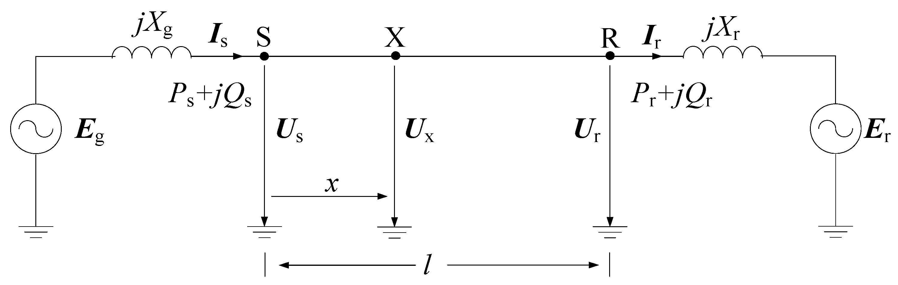
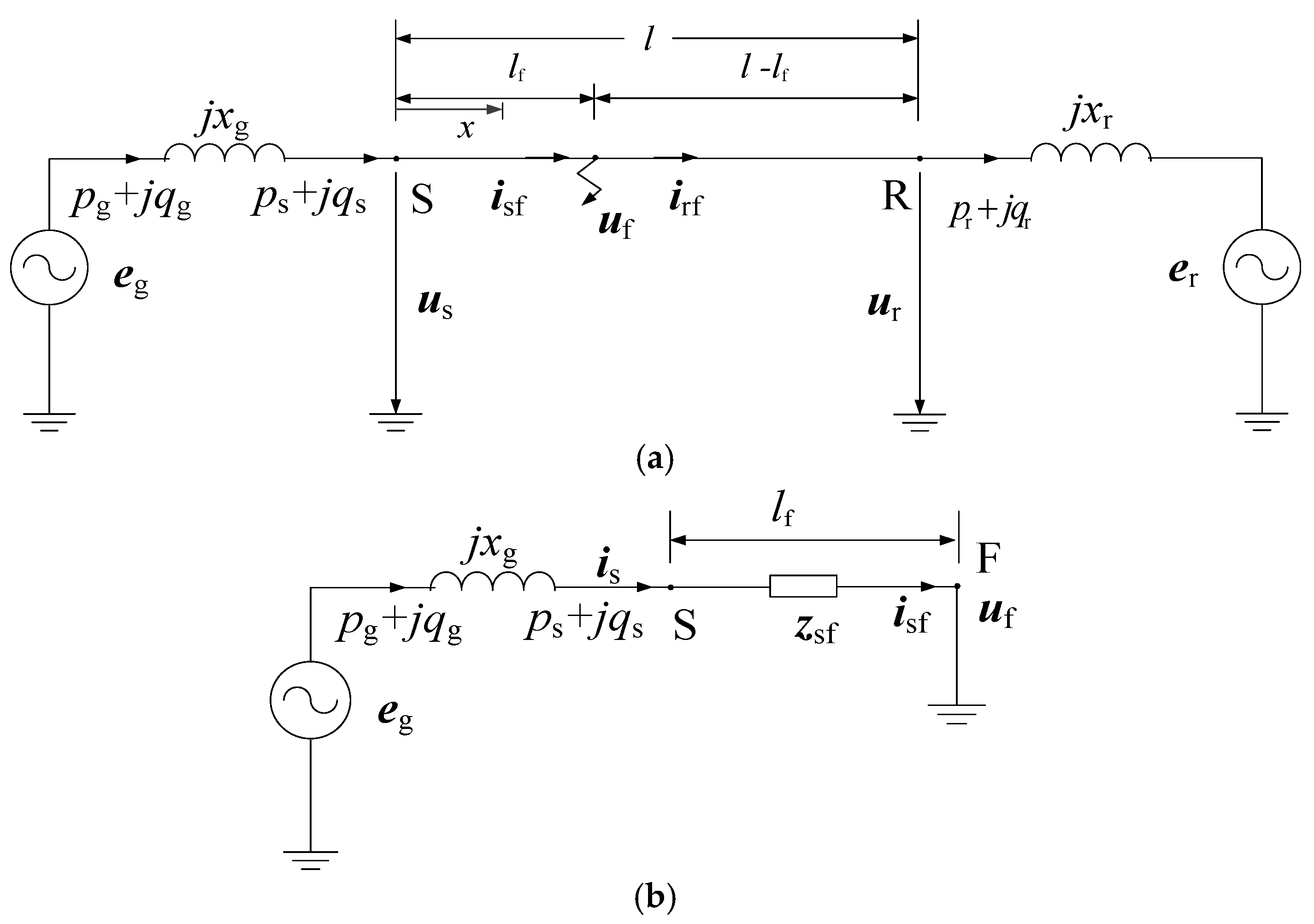
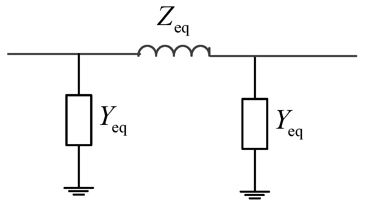
Half-wavelength transmission lines are usually applied in point-to-grid transmission systems or grid-to-grid transmission systems. For both cases, the steady-state characteristics and the synchronization stability of the system can be analyzed by the single-machine-infinite-bus system. When considering the sending-end system and the receiving-end system, a general long-distance transmission system can be represented by Figure 1. The transmission line adopts the positive sequence distributed parameter model; the sending-end generator-transformer unit adopts the classical generator model; the receiving-end system is represented by the Thevenin equivalent circuit.

As shown in Figure 1, E_g and X_g are the equivalent electromotive force and the equivalent impedance of the sending-end generator-transformer unit; E_r and X_r are the equivalent source voltage and the equivalent impedance of the receiving-end system. U_s and U_r are the voltages at both ends of the transmission line. I_s and I_r are the currents of the sending end and receiving end. U_x is the voltage at the point x km away from the sending end. l is the length of the transmission line (or called the transmission distance). P_s and Q_s are the active and reactive power of the sending end; P_r and Q_r are the active and reactive power of the receiving end.

When taking the line resistance into consideration, the basic characteristic of the transmission line is described by the long line equations:

$${\mathit{U}}_{\mathrm{r}}={\mathit{U}}_{\mathrm{s}}\mathrm{ch}\gamma l-{\mathit{I}}_{\mathrm{s}}{\mathit{Z}}_{\mathrm{C}}\mathrm{sh}\gamma l$$

(1)

$${\mathit{I}}_{\mathrm{r}}=-{\mathit{U}}_{\mathrm{s}}\mathrm{sh}\gamma l/{\mathit{Z}}_{\mathrm{C}}+{\mathit{I}}_{\mathrm{s}}\mathrm{ch}\gamma l$$

(2)

where Z_C is the line’s surge impedance; γ is the line’s propagation coefficient. Z_C and γ can be calculated by:

$${\mathit{Z}}_{\mathrm{C}}=\sqrt{\left(R_1+j\omega L_1\right)/\left(G_1+j\omega C_1\right)}$$

(3)

$$\gamma =\alpha +j\beta =\sqrt{\left(R_1+j\omega L_1\right)\left(G_1+j\omega C_1\right)}$$

(4)

where R₁, L₁, G₁, and C₁ are the positive sequence resistance, inductance, conductance, and capacitance of per unit length, respectively; ω is the angular frequency; α is the attenuation constant and β is the phase constant.

To facilitate the description of system characteristics and to carry out numerical calculations, a test system is analyzed in this paper. The rated frequency of the system is supposed to be 50 Hz. The unit length line parameters are given by [17,18], and the surge impedance and the propagation coefficient are calculated by (3) and (4). Detailed parameters are shown in

Table 1. Transmission Line Parameters.

Items		Values
Unit length line parameters	Resistance	0.00801 Ω/km
	Reactance	0.83747 mH/km
	Conductance	0 S/km
	Capacitance	0.01383 μF/km
Propagation coefficient	Attenuation constant (α)	1.6273 × 10−5 km−1
	Phase constant (β)	1.06929 × 10−3 km−1
Surge impedance (ZC)		246.135 ∠ −0.87° Ω

.

As shown in Table 1, the attenuation constant (α) is much smaller than the phase constant (β); the phase angle of the surge impedance is negligible. These system parameters are very close to those of lossless lines.

The half wavelength of the test system is:

$$\lambda /2=\mathsf{\pi }/\beta =2938.0\mathrm{km}$$

(5)

The rated voltage of the line (U_rated) is supposed to be 1000 kV, and then the surge impedance loading is:

$$P_{\mathrm{SIL}}=U_{\mathrm{rated}}^2/\left|{\mathit{Z}}_C\right|=4062.8\mathrm{MW}$$

(6)

In this paper, the rated voltage and the surge impedance loading of the transmission line are set as the reference voltage (U_B) and the reference capacity (S_B) for the per-unit system, respectively. The actual values of physical quantities are represented by upper-case letters, and the corresponding per-unit values are represented by lower-case letters in this paper.

In order to analyze the typical application of half wavelength transmission system in transmitting bulk power from energy bases to the load centers, assume the parameters of the two end systems are as shown in

Table 2. Parameters of the sending-end and the receiving-end systems.

Items		Values
Sending end system	Rated capacity of the generator	2 × SIL
	Subtransient reactance of the generator	0.1 p.u.
	Rated capacity of the transformer	2 × SIL
	Leakage inductances of the transformer	0.1 p.u.
	Equivalent impedance of the sending-end system (xg)	0.2 p.u.
Receiving-end system	Short circuit capacity of the receiving-end system	20 × SIL
	Equivalent impedance of the receiving -end system (xr)	0.05 p.u.

.

First we neglect the losses of the transmission line, according to the long line equations and Figure 1, we have:

$$\left[\begin{array}{c}{\mathit{i}}_{\mathrm{s}}\\ -{\mathit{i}}_{\mathrm{r}}\end{array}\right]=\left[\mathit{y}\right]\left[\begin{array}{c}{\mathit{e}}_{\mathrm{g}}\\ {\mathit{e}}_{\mathrm{r}}\end{array}\right]$$

(7)

where the admittance matrix [y] is:

$$\left[\mathit{y}\right]=\frac{1}{{\Delta }_0}\left[\begin{array}{cc}j\left(x_{\mathrm{r}}\sin \left(\beta l\right)-\cos \left(\beta l\right)\right)& j\\ j& j\left(x_{\mathrm{g}}\sin \left(\beta l\right)-\cos \left(\beta l\right)\right)\end{array}\right]$$

(8)

$${\Delta }_0=(1-x_{\mathrm{g}}{x}_{\mathrm{r}})\sin \left(\beta l\right)+(x_{\mathrm{g}}+x_{\mathrm{r}})\cos \left(\beta l\right)$$

(9)

According to (7), the following per-unit power equations can be derived:

$$p_{\mathrm{g}}=p_{\mathrm{r}}=\frac{e_{\mathrm{g}}{e}_{\mathrm{r}}\sin {\delta }_{\mathrm{g}}}{{\Delta }_0}$$

(10)

$$q_{\mathrm{g}}=\frac{e_{\mathrm{g}}\left(-e_{\mathrm{r}}\cos \left({\delta }_{\mathrm{g}}\right)-e_{\mathrm{g}}{x}_{\mathrm{r}}\sin (\beta l)+e_{\mathrm{g}}\cos (\beta l)\right)}{{\Delta }_0}$$

(11)

$$q_{\mathrm{r}}=\frac{e_{\mathrm{r}}\left(e_{\mathrm{g}}\cos \left({\delta }_{\mathrm{g}}\right)+e_{\mathrm{r}}{x}_{\mathrm{g}}\sin \left(\beta l\right)-e_{\mathrm{r}}\cos \left(\beta l\right)\right)}{{\Delta }_0}$$

(12)

where δ_g is the phase angle difference between e_g and e_r.

Similarly, if the line losses are considered, the power equations become:

$$p_{\mathrm{g}}=\frac{C_1\sin {\delta }_{\mathrm{g}}+C_2\cos {\delta }_{\mathrm{g}}+C_3}{{\Delta }_{\mathrm{loss}}}=\frac{K_1\sin \left({\delta }_{\mathrm{g}}+{\phi }_1\right)+C_3}{{\Delta }_{\mathrm{loss}}}$$

(13)

$$q_{\mathrm{g}}=\frac{C_2\sin {\delta }_{\mathrm{g}}-C_1\cos {\delta }_{\mathrm{g}}+C_4}{{\Delta }_{\mathrm{loss}}}=\frac{K_1\sin \left({\delta }_{\mathrm{g}}+{\phi }_2\right)+C_4}{{\Delta }_{\mathrm{loss}}}$$

(14)

$$p_{\mathrm{r}}=\frac{C_1\sin {\delta }_{\mathrm{g}}-C_2\cos {\delta }_{\mathrm{g}}+C_5}{{\Delta }_{\mathrm{loss}}}=\frac{K_1\sin \left({\delta }_{\mathrm{g}}+{\phi }_3\right)+C_5}{{\Delta }_{\mathrm{loss}}}$$

(15)

$$q_{\mathrm{r}}=\frac{C_2\sin {\delta }_{\mathrm{g}}+C_1\cos {\delta }_{\mathrm{g}}+C_6}{{\Delta }_{\mathrm{loss}}}=\frac{K_1\sin \left({\delta }_{\mathrm{g}}+{\phi }_4\right)+C_6}{{\Delta }_{\mathrm{loss}}}$$

(16)

where:

$$K_1=\sqrt{C_1{}^2+C_2{}^2}$$

(17)

$${\Delta }_{\mathrm{loss}}={\left|\left(x_{\mathrm{g}}{x}_{\mathrm{r}}-{\mathrm{z}}_{\mathrm{c}}{}^2\right)\mathrm{sh}\gamma l-j{\mathrm{z}}_{\mathrm{c}}\left(x_{\mathrm{g}}+x_{\mathrm{r}}\right)\mathrm{ch}\gamma l\right|}^2$$

(18)

When the transmission line parameters and x_g, x_r, e_g, e_r are given, C1–C6 and ${\phi }_1$–${\phi }_4$ are constants. The detail expressions are given in the Appendix A.1.

3. Resonant Transmission Distance

Using (9), we have:

$${\Delta }_0=\sqrt{{(x_{\mathrm{g}}+x_{\mathrm{r}})}^2+{(1-x_{\mathrm{g}}{x}_{\mathrm{r}})}^2}\sin \left(\beta l+{\phi }_{\mathrm{C}}\right)$$

(19)

where:

$${\phi }_{\mathrm{C}}=\arctan \frac{x_{\mathrm{g}}+x_{\mathrm{r}}}{1-x_{\mathrm{g}}{x}_{\mathrm{r}}}\in \left(0，\frac{\mathsf{\pi }}{2}\right)$$

(20)

When $l=\left(\mathsf{\pi }-{\phi }_{\mathrm{C}}\right)/\beta$, Δ₀ = 0. Then according to (8), the denominators of elements in the admittance matrix [y] are zero. Series resonance occurs between the transmission line and the equivalent reactance of both sides of the system. If we define the transmission distance at this condition as the resonant transmission distance and denote it as l_resnt, then we have:

$$l_{\mathrm{resnt}}=\left[\arctan \left(\frac{x_{\mathrm{r}}+x_g}{x_{\mathrm{r}}{x}_g-1}\right)+\mathsf{\pi }\right]/\beta$$

(21)

As shown in (21), l_resnt is dependent on the parameters of the transmission line and the equivalent reactance of both ends, but not related to e_g and e_r.

When the losses of the transmission line are considered, the resonant transmission distance can also be calculated by (21) according to (18). For the test system, l_resnt is about 2707 km, βl_resnt is about 165.8°.

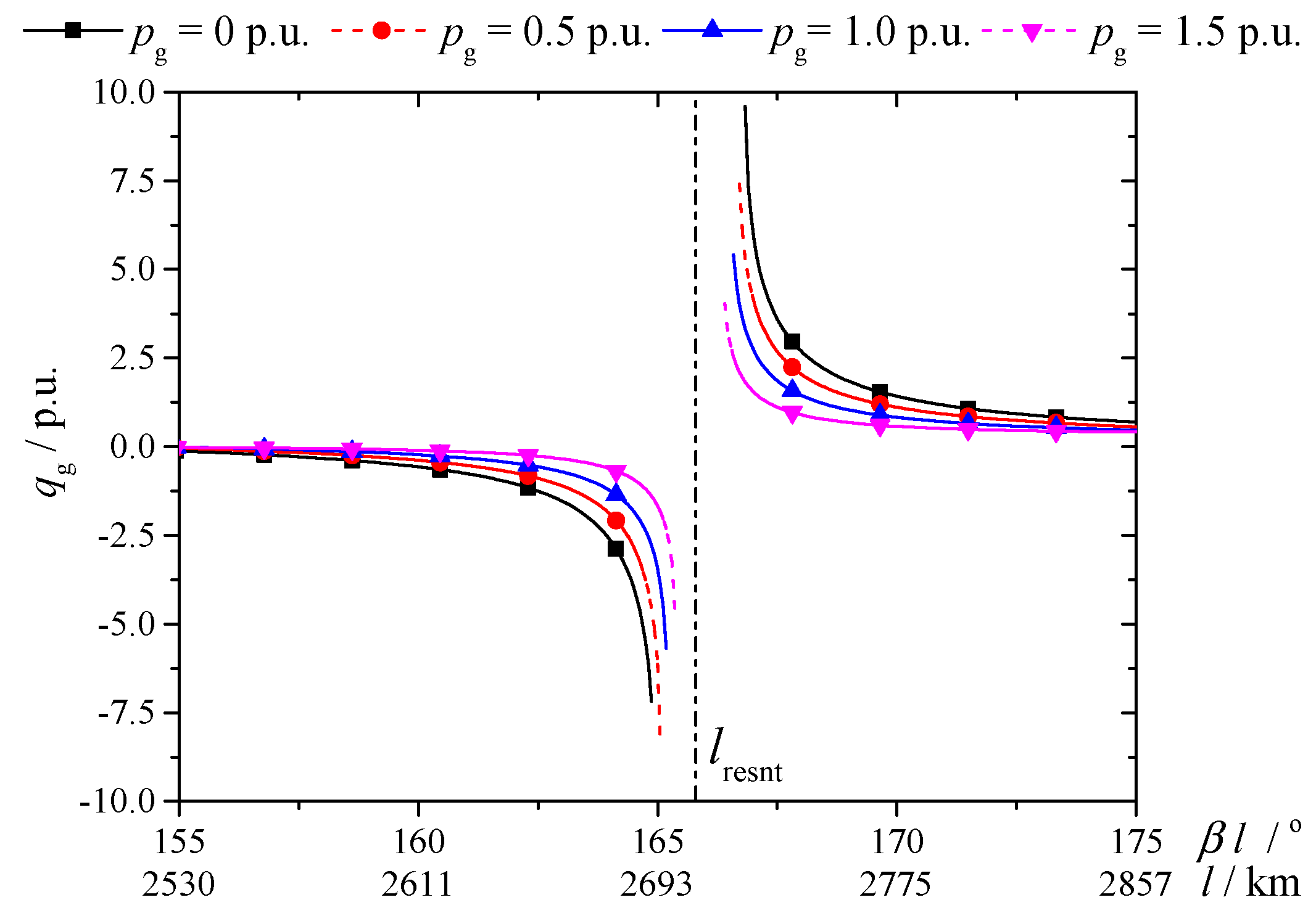
To analyze the test system’s characteristic, we set a general terminal condition, which is e_g = 1.1 p.u. and e_r = 1.0 p.u. Then q_g is calculated under different transmission power and transmission distances, and the results are shown in Figure 2.

As shown in Figure 2, when the transmission distance is close to l_resnt (in 2700–2715 km), there is no solution for (13), so the test system cannot operate; when the transmission distance is not in the above range, the test system can operate, but the absolute value of q_g is too large. For example, when βl = 167°, if p_g = 0 p.u., 0.5 p.u., 1.0 p.u. and 1.5 p.u., then q_g is 5.81 p.u., 4.06 p.u., 2.69 p.u., and 1.53 p.u., respectively. It can be seen that the less the p_g is, the greater the absolute value of the q_g is. With the increase of the deviation between l and l_resnt, q_g decreases; when l reduces to below 2639 km or l increases to over 2804 km, the absolute value of q_g decreases to below 1.0 p.u.

Thereby, the transmission distance should stay away from l_resnt to make the system operational and to decrease the reactive power.

4. Steady-State Overvoltage Analysis

In order to further determine the feasible transmission distance, the steady-state overvoltage is analyzed. According to the long line equations, the voltage at the point x km away from the sending end is:

$${\mathit{u}}_{\mathrm{x}}={\mathit{u}}_{\mathrm{s}}\mathrm{ch}\gamma x-{\mathit{i}}_{\mathrm{s}}{\mathbf{𝔃}}_{\mathrm{C}}\mathrm{sh}\gamma x$$

(22)

where:

$${\mathit{i}}_{\mathrm{s}}={\left[\left(p_g+j{q}_g\right)/{\mathit{e}}_{\mathrm{g}}\right]}^{*}$$

(23)

$${\mathit{u}}_{\mathrm{s}}={\mathit{e}}_{\mathrm{g}}-j{\mathit{i}}_{\mathrm{s}}{x}_{\mathrm{g}}$$

(24)

where * indicates the conjugate complex.

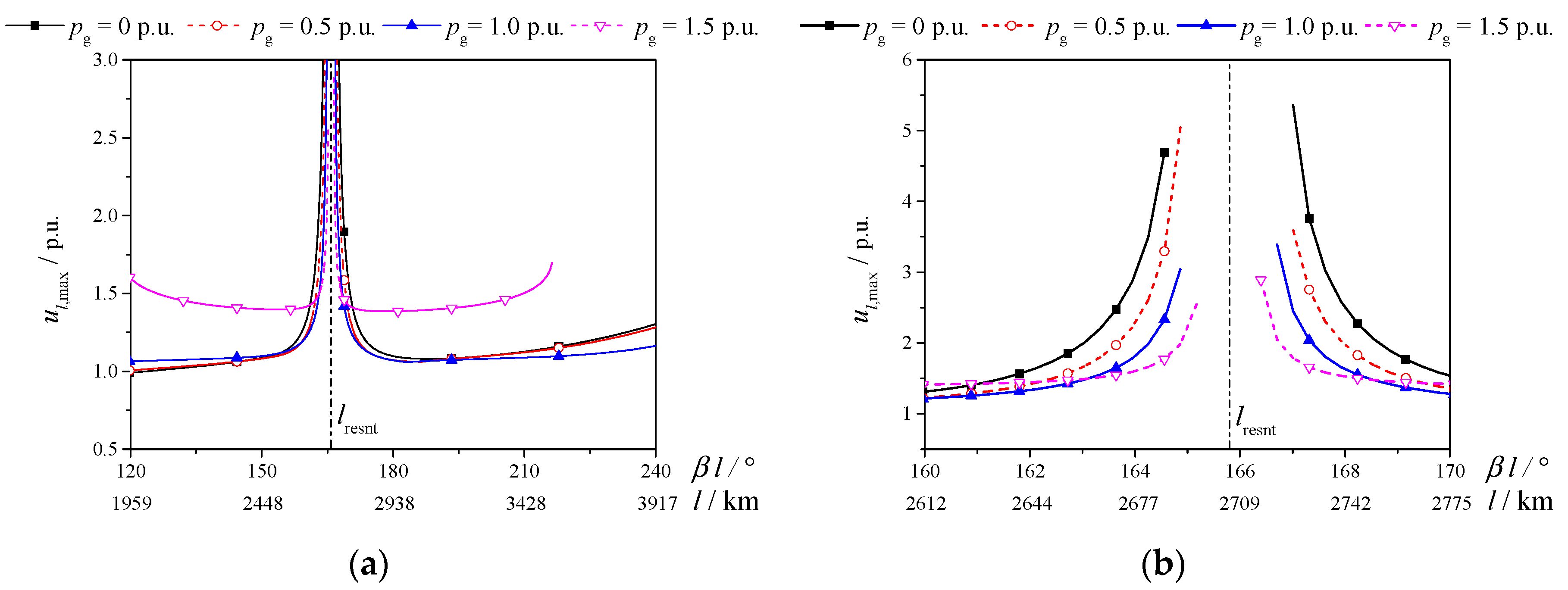
Under the terminal condition e_g = 1.1 p.u. and e_r = 1.0 p.u., taking p_g as a parameter, for different transmission distances, the maximum voltage along the whole transmission line, which is defined as u_l,max, is calculated as shown in Figure 3. Figure 3a is a large range picture of u_l,max in different transmission distances; while Figure 3b is a small range picture of u_l,max for clearer presentation.

From Figure 3, it can be drawn that:

(1)

Under different p_g, when l gets closer to l_resnt, u_l,max has an abrupt increase;

(2)

As shown in Figure 3b, for l in the range of 163.3°–164.6° and 167.0°–168.2°, u_l,max decreases with the increase of p_g;

(3)

As shown in Figure 3a, when p_g is 1.5 p.u., there is obvious overvoltage for all the transmission distances and u_l,max is close to p_g for most transmission distances. Actually, this is true for any transmission power larger than 1.0 p.u.

(4)

As shown in Figure 3a, there is no operation point when p_g is 1.5 p.u. and βl is larger than 217.1°; similarly, as shown in Figure 3b, there is no operation point when p_g is 0.0 p.u. and βl is in the range of 164.6°–167.0°.

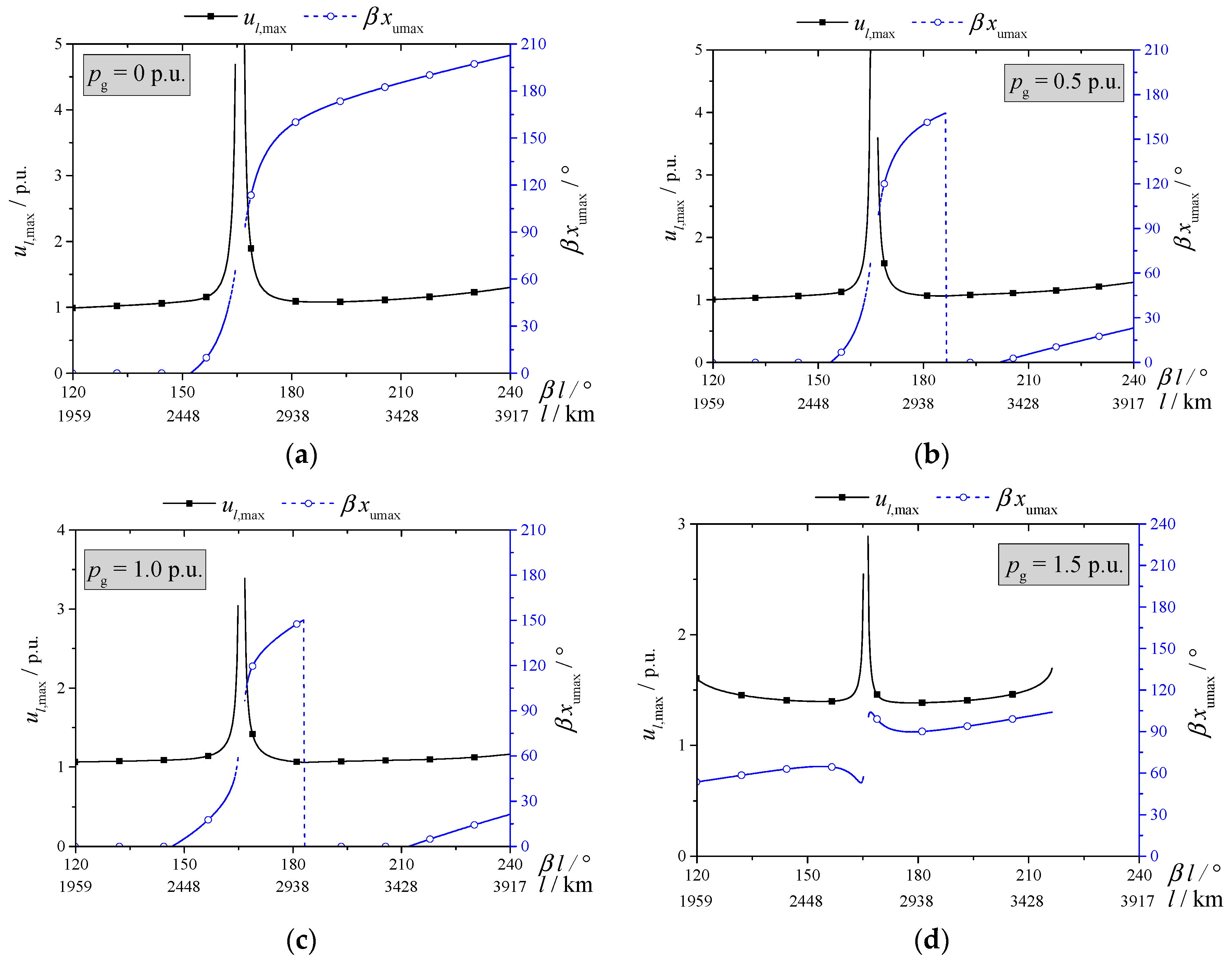
Figure 3 only gives the maximum voltage along the whole line, we still need to know the location where the maximum voltage occurs. The location where the maximum voltage (u_l,max) occurs is defined as x_umax (in km) or βx_umax (in deg.). The maximum voltage (u_l,max) and its location (βx_umax) for different transmission distances with fixed transmission power are illustrated in Figure 4 and described in

Table 3. Description of specified points in Figure 4.

Transmission Power pg/p.u.	Transmission Distance		The Maximum Voltage ul,max/p.u.	The Maximum Voltage Location
	βl/°	l/km		βxumax/°	xumax/km
0	150	2448.3	1.086	0	0
	167	2725.8	5.357	90.3	1473.9
	180	2938.0	1.099	158.1	2580.5
	210	3427.7	1.126	185.2	3022.9
0.5	150	2448.3	1.081	0	0
	167	2725.8	3.595	96.0	1566.9
	180	2938.0	1.072	159.5	2603.4
	210	3427.7	1.121	5.5	89.8
1.0	150	2448.3	1.098	5.4	88.1
	167	2725.8	2.446	103.1	1682.8
	180	2938.0	1.071	145.7	2378.1
	210	3427.7	1.088	0	0
1.5	150	2448.3	1.399	64.3	1049.5
	167	2725.8	1.787	104.1	1699.1
	180	2938.0	1.385	89.9	1467.4
	210	3427.7	1.501	101.0	1648.5

.

As shown in Figure 4 and Table 3, taking p_g = 1.0 p.u for example, when the transmission distance is 2448.3 km (150°), 2725.8 km (167°), 2938.0 km (180°), and 3427.7 km (210°), respectively, the maximum voltage along the transmission line (u_l,max) is 1.098 p.u., 2.446 p.u., 1.071 p.u., and 1.088 p.u., respectively, and the location where the maximum voltage occurs (x_umax or βx_umax) is 88.1 km (5.4°), 1682.8 km (103.1°), 2378.1 km (145.7°), and 0.0 km (0°), respectively.

If we choose u_l,max < 1.5 p.u. as the permissible range of overvoltage, when p_g changes from 0 p.u. to 1.5 p.u., the feasible range of transmission distance for the test system is:

$$\{\begin{array}{l}{126.0}^{\circ }<\beta l<{161.5}^{\circ }\\ {170.1}^{\circ }<\beta l<{210.0}^{\circ }\end{array}$$

(25)

5. Small Signal Synchronization Stability Analysis

The rotor motion equation of the system is:

$$\{\begin{array}{l}\frac{d{\delta }_{\mathrm{g}}}{dt}={\omega }_0\cdot ({\omega }_{\mathrm{g}}-1)\\ \frac{d{\omega }_{\mathrm{g}}}{dt}=\frac{1}{2H}(p_{\mathrm{m}}-p_{\mathrm{g}}-D\cdot ({\omega }_{\mathrm{g}}-1))\end{array}$$

(26)

where ω₀, ω_g, H, p_m, and D are the rated angular frequency of the system, the angular frequency of the generator, the inertia time constant, the mechanical power and the damping coefficient of the generator, respectively. When p_m is supposed to be constant, the linearized equation of the rotor motion equation at the operating point (δ_g⁽⁰⁾, ω₀) is:

$$\left[\begin{array}{c}\frac{d\Delta {\delta }_{\mathrm{g}}}{dt}\\ \frac{d\Delta {\omega }_{\mathrm{g}}}{dt}\end{array}\right]=\left[\begin{array}{cc}0& {\omega }_0\\ -\frac{K_1\cos \left({\delta }_{\mathrm{g}}^{(0)}+{\phi }_1\right)}{2H{\Delta }_{\mathrm{loss}}}& -\frac{D}{2H}\end{array}\right]\left[\begin{array}{c}\Delta {\delta }_{\mathrm{g}}\\ \Delta {\omega }_{\mathrm{g}}\end{array}\right]$$

(27)

where K₁, Δ_loss and ${\phi }_1$ have been defined in (13)–(18).

The characteristic equation of the system is:

$${\lambda }^2+\frac{D}{2H}\lambda +\frac{{\omega }_0}{2H}\frac{K_1}{{\Delta }_{\mathrm{loss}}}\cos \left({\delta }_{\mathrm{g}}^{(0)}+{\phi }_1\right)=0$$

(28)

Because H and D are positive, the small signal synchronization stability condition of the system finally becomes:

$$K_{\mathrm{synch}}=\frac{K_1}{{\Delta }_{\mathrm{loss}}}\cos \left({\delta }_g^{(0)}+{\phi }_1\right)>0$$

(29)

We define K_synch as the synchronization coefficient. The characteristic of the half-wavelength transmission system can be summarized as: if K_synch is positive, the system is stable under small disturbances; otherwise, the system is unstable. For the test system with the terminal condition of e_g = 1.1 p.u. and e_r = 1.0 p.u., the synchronization coefficient are calculated under different transmission distances with fixed transmission power p_g. The results are shown in Figure 5 and described in

Table 4. Description of specified points in Figure 4.

Transmission Distance		Transmission Power pg/p.u.	Synchronization Coefficient Ksynch
βl/°	l/km
150	2448.3	0	−3.88
		0.5	−3.91
		1.0	−3.88
		1.5	−3.78
167	2725.8	0	4.65
		0.5	6.69
		1.0	8.21
		1.5	9.46
180	2938.0	0	4.24
		0.5	4.31
		1.0	4.33
		1.5	4.29
210	3427.7	0	1.53
		0.5	1.50
		1.0	1.28
		1.5	0.74

.

As shown in Figure 5 and Table 4, taking βl = 150° for example, when p_g = 0 p.u., 0.5 p.u., 1.0 p.u., and 1.5 p.u., respectively, K_synch = −3.88, −3.91, −3.88 and −3.78 respectively. From Figure 5 we can see: in the studied transmission distance range, when l is smaller than l_resnt, K_synch is negative; and when l is greater than l_resnt, e.g., βl = 167°, K_synch becomes positive. So, only when l is larger than l_resnt, may the system be stable. Considering the small signal synchronization stability condition of the test system, when p_g changes from 0 p.u. to 1.5 p.u., the feasible transmission distance range is:

$${166.8}^{\circ }<\beta l<{217.1}^{\circ }$$

(30)

6. Feasible Transmission Distance Analysis

Taking the overvoltage constraint (25) and the small signal synchronization stability constraint (30) into consideration, when p_g changes from 0 p.u. to 1.5 p.u., the feasible range of the transmission distance for the half-wavelength transmission system is:

$${170.1}^{\circ }<\beta l<{210.0}^{\circ }$$

(31)

In considering of the frequency variation during transient process, we set an allowable frequency variation range of −3% to +3% of the rated frequency. βl changes with the variation of frequency, as shown in Figure 6.

As shown in Figure 6, when the frequency changes −3%, the feasible transmission distance range for the half-wavelength transmission system is:

$$2862.3\mathrm{km}<l<3533.7\mathrm{km}$$

(32)

When the frequency changes 3%, the feasible range is:

$$2695.6\mathrm{km}<l<3327.9\mathrm{km}$$

(33)

In conclusion, after considering the frequency variation, the feasible transmission distance range that satisfies both the overvoltage constraint and the synchronization stability constraint is:

$$2862.3\mathrm{km}<l<3327.9\mathrm{km}$$

(34)

7. Transient Overvoltage Analysis

This section studies the transient overvoltage characteristic under three-phase short circuit faults. The test system and the transient model mentioned in Section 2 are adopted. The transmission distance is supposed to be in the feasible range given by (34). The system is in the steady state at t = 0−, and the fault occurs at t = 0+. The system model under the three-phase short circuit fault is shown in Figure 7.

In Figure 7, all the per-unit values in lower-case letters are based on SIL and the rated voltage of the transmission line. The meanings of the variables in Figure 7 are the same as in Figure 1. Besides, l_f is the distance between the fault point and the sending end; u_f is the voltage of the fault point; i_sf and i_rf are the currents of the fault point; z_sf is the input impedance seen from the sending end.

When the phase angle of Z_c is ignored, using u_f = 0 and the long line equations, we can deduce:

$$\{\begin{array}{l}{\mathit{u}}_{\mathrm{s}}={\mathit{u}}_{\mathrm{f}}\mathrm{ch}\left(\gamma l_{\mathrm{f}}\right)+{\mathit{i}}_{\mathrm{s}}{\mathit{u}}_{\mathrm{f}}\mathrm{sh}\left(\gamma l_{\mathrm{f}}\right)={\mathit{i}}_{\mathrm{s}\mathrm{f}}\mathrm{sh}\left(\gamma l_{\mathrm{f}}\right)\\ {\mathit{i}}_{\mathrm{s}}={\mathit{u}}_{\mathrm{f}}\mathrm{sh}\left(\gamma l_{\mathrm{f}}\right)+{\mathit{i}}_{\mathrm{s}\mathrm{f}}\mathrm{ch}\left(\gamma l_{\mathrm{f}}\right)={\mathit{i}}_{\mathrm{s}\mathrm{f}}\mathrm{ch}\left(\gamma l_{\mathrm{f}}\right)\end{array}$$

(35)

Then, the input impedance z_sf can be expressed as:

$${\mathit{z}}_{\mathrm{sf}}={\mathit{u}}_{\mathrm{s}}/{\mathit{i}}_{\mathrm{s}}=\mathrm{th}\left(\gamma l_{\mathrm{f}}\right)$$

(36)

During the fault period, the magnitude of e_g is constant. According to (36) and the sending end equivalent circuit shown in Figure 7b, u_s and i_s can be expressed as:

$$\{\begin{array}{l}{\mathit{u}}_{\mathrm{s}}={\mathit{e}}_{\mathrm{g}}{\mathit{z}}_{\mathrm{sf}}/\left({\mathit{z}}_{\mathrm{sf}}+j{x}_{\mathrm{g}}\right)\\ {\mathit{i}}_{\mathrm{s}}={\mathit{e}}_{\mathrm{g}}/\left({\mathit{z}}_{\mathrm{sf}}+j{x}_{\mathrm{g}}\right)\end{array}$$

(37)

According to the long line equations and (37), we can calculate u_x by:

$${\mathit{u}}_{\mathrm{x}}={\mathit{u}}_{\mathrm{s}}\mathrm{ch}\gamma x-{\mathit{i}}_{\mathrm{s}}\mathrm{sh}\gamma x=\frac{{\mathit{e}}_{\mathrm{g}}\left(\mathrm{th}\gamma l_{\mathrm{f}}\mathrm{ch}\gamma x-\mathrm{sh}\gamma x\right)}{\mathrm{th}\gamma l_{\mathrm{f}}+j{x}_{\mathrm{g}}}$$

(38)

Then the magnitude of u_x is:

$$u_{\mathrm{x}}=\frac{e_{\mathrm{g}}}{\left|\mathrm{th}\gamma l_{\mathrm{f}}+j{x}_{\mathrm{g}}\right|}\left|\mathrm{th}\gamma l_{\mathrm{f}}\mathrm{ch}\gamma x-\mathrm{sh}\gamma x\right|$$

(39)

It can be proved that when the imaginary part of (thγl_f + jx_g) is zero, u_x will get its maximum value u_fmax. So we define l_fmax as the solution of the equation Im(thγl_fmax + jx_g) = 0, whose meaning is the fault distance which will cause the largest overvoltage compared to the other fault distance. After l_fmax is defined, we next define the location at which the maximum overvoltage occurs, which is defined as x_f,umax. The meaning of x_f,umax is: when a three phase fault occurs at l_fmax, the maximum overvoltage u_fmax will occur at x_f,umax. According to the definitions of u_fmax, l_fmax, and x_f,umax, we can derive their expressions from (39) as:

$$l_{\mathrm{f}\max }=\left[\pi -\arctan \left(x_{\mathrm{g}}\right)\right]/\beta$$

(40)

$$x_{\mathrm{f},\mathrm{umax}}=l_{\mathrm{fmax}}-\mathsf{\pi }/\left(2\beta \right)$$

(41)

$$u_{f\max }\approx \frac{e_{\mathrm{g}}}{\mathrm{th}(\alpha l_{\mathrm{fmax}})\sqrt{(1+x_{\mathrm{g}}{}^2)}}$$

(42)

It is shown by (40) that l_fmax is shorter than the half wavelength, and it is independent of e_g and e_r. For the test system, βl_fmax is about 168.7°, which is smaller than any feasible transmission distance given by (34). This means that there is always a fault point on the transmission line that will cause the maximum overvoltage.

According to (41), the maximum overvoltage occurs at the point exactly a quarter wavelength away from the fault point.

Using (42), we can estimate the maximum overvoltage u_fmax. Because $e_{\mathrm{g}}\approx 1$, $\mathrm{th}(\alpha l_{\mathrm{fmax}})<\mathrm{th}(0.05)\approx 0.05$ and x_g < 1, $u_{f\max }>20/\sqrt{2}>10$ p.u. So the power-frequency overvoltage is larger than 10 p.u. for the test system. Actually, such a serious overvoltage is unacceptable in the actual power system.

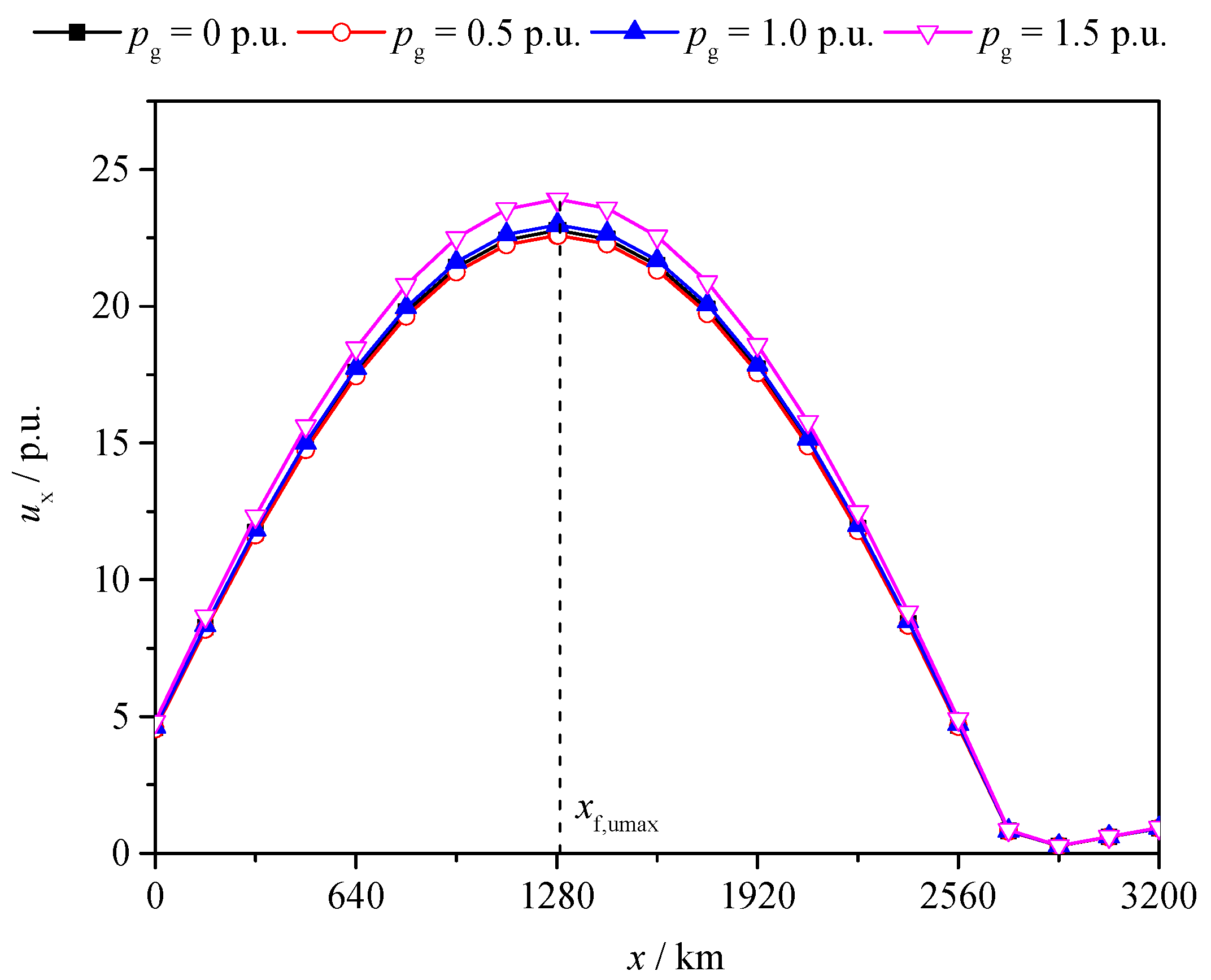
Simulations have been done by PSS/E to illustrate the above conclusion. The structure of the test system is shown in Figure 1. The system parameters given in Section 2 are adopted. The transmission distance is 3200 km. From the sending end of line, a voltage measurement point is set every 160 km, and is numbered from 0 to 20. According to the previous analysis, when the fault point is 2753.4 km away from the sending end (i.e., l_fmax = 2753.4 km), the maximum overvoltage (u_fmax) will occur at the point 1284.4 km away from the sending end (i.e., x_f,umax = 1284.4 km), which is near the 8th measurement point (which is 1280 km away from the sending end).

When the above fault occurs, the voltage profile of the line is shown in Figure 8.

As shown in Figure 8, when p_g = 0 p.u., 0.5 p.u., 1.0 p.u., and 1.5 p.u., respectively, the maximum overvoltage is 22.77 p.u., 22.59 p.u., 22.98 p.u., and 23.91 p.u., respectively. This example illustrates that the maximum overvoltage (u_fmax) is much larger than 10 p.u., which cannot be accepted in real engineering.

8. Transient Synchronization Stability Analysis

During the fault period, the power of the sending end can be calculated by:

$$p_{\mathrm{s}}+j{q}_{\mathrm{s}}={\mathit{u}}_{\mathrm{s}}{\mathit{i}}_{\mathrm{s}}{}^{*}={\mathit{z}}_{\mathrm{sf}}{\mathit{i}}_{\mathrm{s}}{\mathit{i}}_{\mathrm{s}}{}^{*}={\mathit{z}}_{\mathrm{sf}}{\left|{\mathit{i}}_{\mathrm{s}}\right|}^2=\mathrm{th}\left(\gamma l_{\mathrm{f}}\right)\frac{e_{\mathrm{g}}{}^2}{{\left|\mathrm{th}\gamma l_{\mathrm{f}}+j{x}_{\mathrm{g}}\right|}^2}$$

(43)

According to (43), the electromagnetic power of the sending-end generator is not varied with time during the fault period. We denote it by p_s⁽¹⁾. When l_f = l_fmax, p_s⁽¹⁾ gets its maximum value p_smax⁽¹⁾:

$$p_{\mathrm{smax}}^{(1)}\approx \frac{e_{\mathrm{g}}^2}{\mathrm{th}(\alpha l_{\mathrm{fmax}})\cdot (1+x_{\mathrm{g}}^2)}$$

(44)

Because when l_f = l_fmax, both p_s⁽¹⁾ and u_x get their maximum values, we define l_fmax as the most serious fault point. Using (44), we can estimate the maximum electromagnetic power. Because $e_{\mathrm{g}}\approx 1$, $\mathrm{th}(\alpha l_{\mathrm{fmax}})<\mathrm{th}(0.05)\approx 0.05$ and x_g < 1, so $p_{\mathrm{smax}}^{(1)}>10$ p.u.

During the fault period, the rotor motion equation is:

$$\{\begin{array}{l}\frac{d{\delta }_{\mathrm{g}}}{dt}={\omega }_0\cdot ({\omega }_{\mathrm{g}}-1)\\ \frac{d{\omega }_{\mathrm{g}}}{dt}=\frac{1}{2H}(p_{\mathrm{m}}-p_{\mathrm{s}}{}^{\left(1\right)}-D\cdot ({\omega }_{\mathrm{g}}-1))\end{array}$$

(45)

If the effect of the governor is ignored, p_m = p_s⁽⁰⁾, where p_s⁽⁰⁾ is the electromagnetic power of the steady state. For the convenience of analysis, D is supposed to be zero. If the fault is cleared at time t_clear, the states at the fault clearing time can be calculated by:

$$\{\begin{array}{l}{\omega }_{\mathrm{g}}{}^{\left(1\right)}=\frac{1}{2H}\left(p_{\mathrm{s}}{}^{\left(0\right)}-p_{\mathrm{s}}{}^{\left(1\right)}\right)t_{\mathrm{clear}}+{\omega }_{\mathrm{g}}{}^{\left(0\right)}\\ {\delta }_{\mathrm{g}}{}^{\left(1\right)}=\left(p_{\mathrm{s}}{}^{\left(0\right)}-p_{\mathrm{s}}{}^{\left(1\right)}\right){\omega }_0{t}_{\mathrm{clear}}{}^2/\left(4H\right)+{\delta }_{\mathrm{g}}{}^{\left(0\right)}\end{array}$$

(46)

where ω_g⁽⁰⁾ = 1.0 p.u.; δ_g⁽⁰⁾ is the phase angle difference between e_g and e_r before the fault; ω_g⁽¹⁾ and δ_g⁽¹⁾ are the angular frequency and phase angle difference at the fault clearing time.

Next we analyze the transient synchronization stability under the fault at the most serious fault point l_fmax.

For the fault occurs at l_fmax, the states at the fault clearing time are:

$$\{\begin{array}{l}{\omega }_{\mathrm{g}}{}^{\left(1\right)}=\frac{1}{2H}\left(p_{\mathrm{s}}{}^{\left(0\right)}-p_{\mathrm{smax}}{}^{\left(1\right)}\right)t_{\mathrm{clear}}+{\omega }_{\mathrm{g}}{}^{\left(0\right)}\\ {\delta }_{\mathrm{g}}{}^{\left(1\right)}=\left(p_{\mathrm{s}}{}^{\left(0\right)}-p_{\mathrm{smax}}{}^{\left(1\right)}\right){\omega }_0{t}_{\mathrm{clear}}{}^2/\left(4H\right)+{\delta }_{\mathrm{g}}{}^{\left(0\right)}\end{array}$$

(47)

After the fault is cleared, the system structure recovers. If the losses of the transmission line are ignored, the expression of the generator electromagnetic power is the same as (10):

$$p_{\mathrm{g}}=p_{\mathrm{s}}{}^{\left(2\right)}\approx \frac{e_{\mathrm{g}}{e}_{\mathrm{r}}\sin {\delta }_{\mathrm{g}}}{{\Delta }_0}$$

(48)

where p_s⁽²⁾ is the generator electromagnetic power after the fault is cleared.

According to (48), the electromagnetic power is a sine wave with respect to the power angle of the generator, as shown in Figure 9. During the fault period, the generator gets an initial deceleration area, A₁¯. At the fault clearing time, ω_g⁽¹⁾ is less than ω_g⁽⁰⁾ according to (47), so the phase angle (δ_g) will continue to decrease after the fault is cleared.

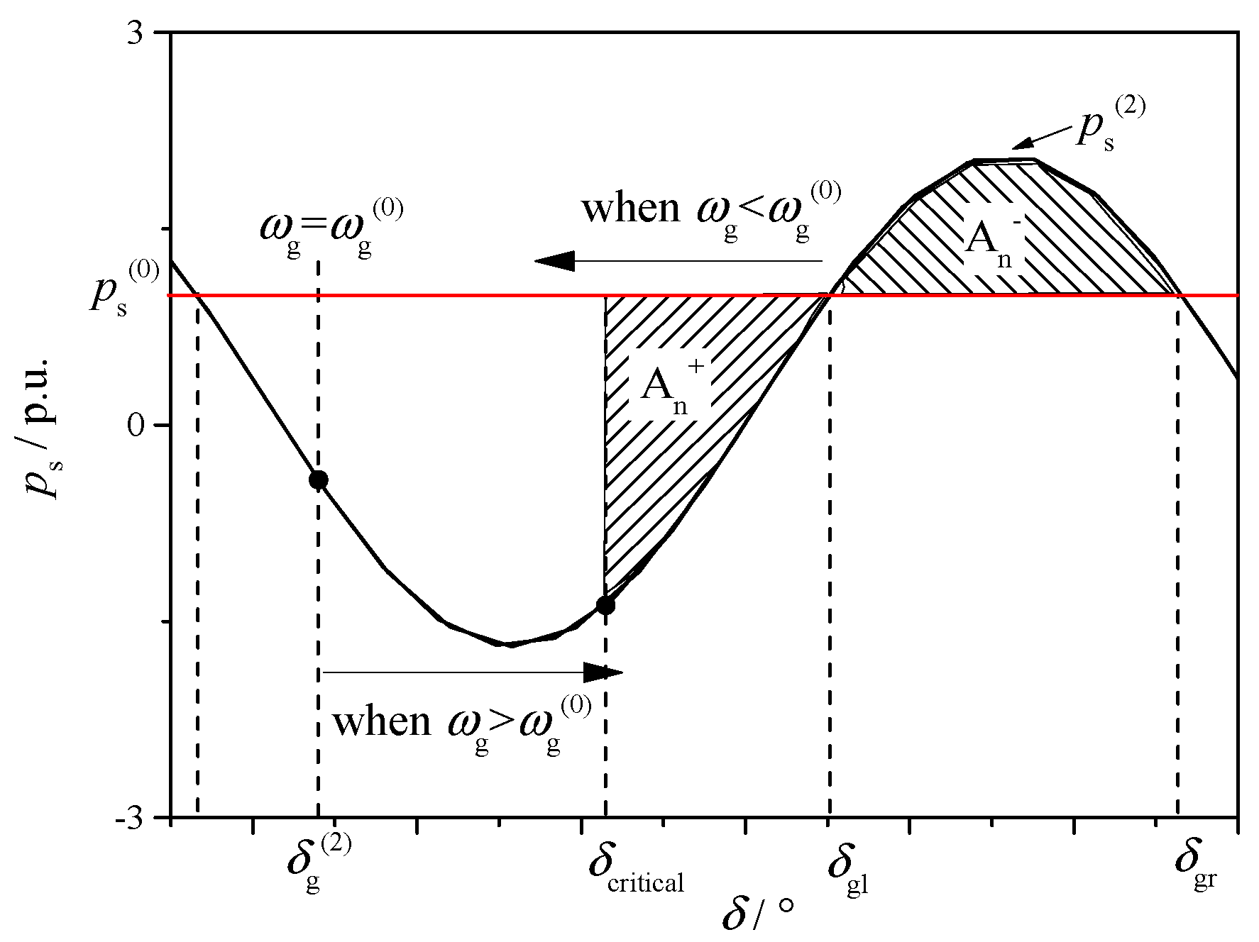
For the fault at l_fmax, because p_smax⁽¹⁾ is much larger than p_s⁽⁰⁾ and the fault clearance requires a certain amount of time, in general, the acceleration area A₁⁺ cannot compensate A₁¯. If the mechanical power of the generator is zero (p_s⁽⁰⁾ = 0), in any sinusoidal cycle of the phase angle, the acceleration area obtained by the generator is always equal to the deceleration area. The phase angle of the generator will keep decreasing after the fault. This means that the system will lose stability after the fault.

If the mechanical power of the generator is positive (p_s⁽⁰⁾ > 0), the acceleration area is always larger than the deceleration area in a sinusoidal cycle of the phase angle, as shown in Figure 10. This means the initial deceleration area (A₁¯) will be compensated gradually. When the initial deceleration area is totally compensated, ω_g will recover to ω_g⁽⁰⁾. Suppose that when δ_g reaches δ_g⁽²⁾, ω_g recovers to ω_g⁽⁰⁾, and the initial deceleration area is totally compensated, then the last compensating area is gotten at δ_g⁽²⁾, this is to say, p_s must be smaller than p_s⁽⁰⁾ when δ_g is at δ_g⁽²⁾.

On the other hand, there is a critical phase angle (δ_critical) that makes A_n⁺ = A_n¯, as shown in Figure 10. Before ω_g recovers to ω_g⁽⁰⁾, δ_g is in the decreasing state. Next we will prove that δ_g⁽²⁾ must be less than δ_critical, i.e., δ_g⁽²⁾ must be on the left of δ_critical.

If δ_g⁽²⁾ > δ_critical, i.e., δ_g⁽²⁾ is on the right of δ_critical, then A_n⁺ cannot compensate A_n⁻, the sum of the deceleration area and the acceleration area will be negative, and ω_g will be still less than ω_g⁽⁰⁾ when δ_g reaches (from right to left) δ_g⁽²⁾. This contradicts to the definition of δ_g⁽²⁾. Thereby, δ_g⁽²⁾ must be less than δ_critical, i.e., δ_g⁽²⁾ must be on the left of δ_critical.

After ω_g increases to ω_g⁽⁰⁾, because δ_g⁽²⁾ is on the left of δ_critical, the acceleration area is always larger than the deceleration area. Then ω_g will always be larger than ω_g⁽⁰⁾, and δ_g is in the increasing state. In this situation, when δ_g reaches δ_gr, ω_g is still larger than ω_g⁽⁰⁾, and δ_g will keep increasing. The system also loses stability after the fault.

In conclusion, the phase angle δ_g will keep decreasing, or keep increasing after a certain time of decreasing. In both cases, the system will lose stability under the fault that occurs at the most serious fault point. Actually, the same conclusion will be obtained through similar derivation process when the losses of the transmission line are considered and the power equation is expressed as (13).

The above result shows that if the sending-end generator is modeled by the classical model, the system will lose stability under the fault that occurs at the most serious fault point.

Simulations have been done to illustrate this conclusion. The test system in Section 7 is adopted. The sending end generator is modeled by the classical model with H = 8.692 p.u. and D = 0. The receiving end system is represented by the Thevenin equivalent circuit with x_r = 0.05 p.u. In the simulations, the short circuit fault occurs at l_fmax at 1 s. The swing curves of the sending-end generator power angle under different fault clearing time (0.03–0.11 s) are shown in Figure 11.

As shown in Figure 11, when p_g⁽⁰⁾ = 0 p.u., δ_g keeps decreasing after the fault. When p_g⁽⁰⁾ = 0.5 p.u., 1.0 p.u. and 1.5 p.u. respectively, δ_g keeps increasing after a certain time of decreasing. For all the cases, the system is unstable after the fault. This is consistent with the conclusion of the previous analysis.

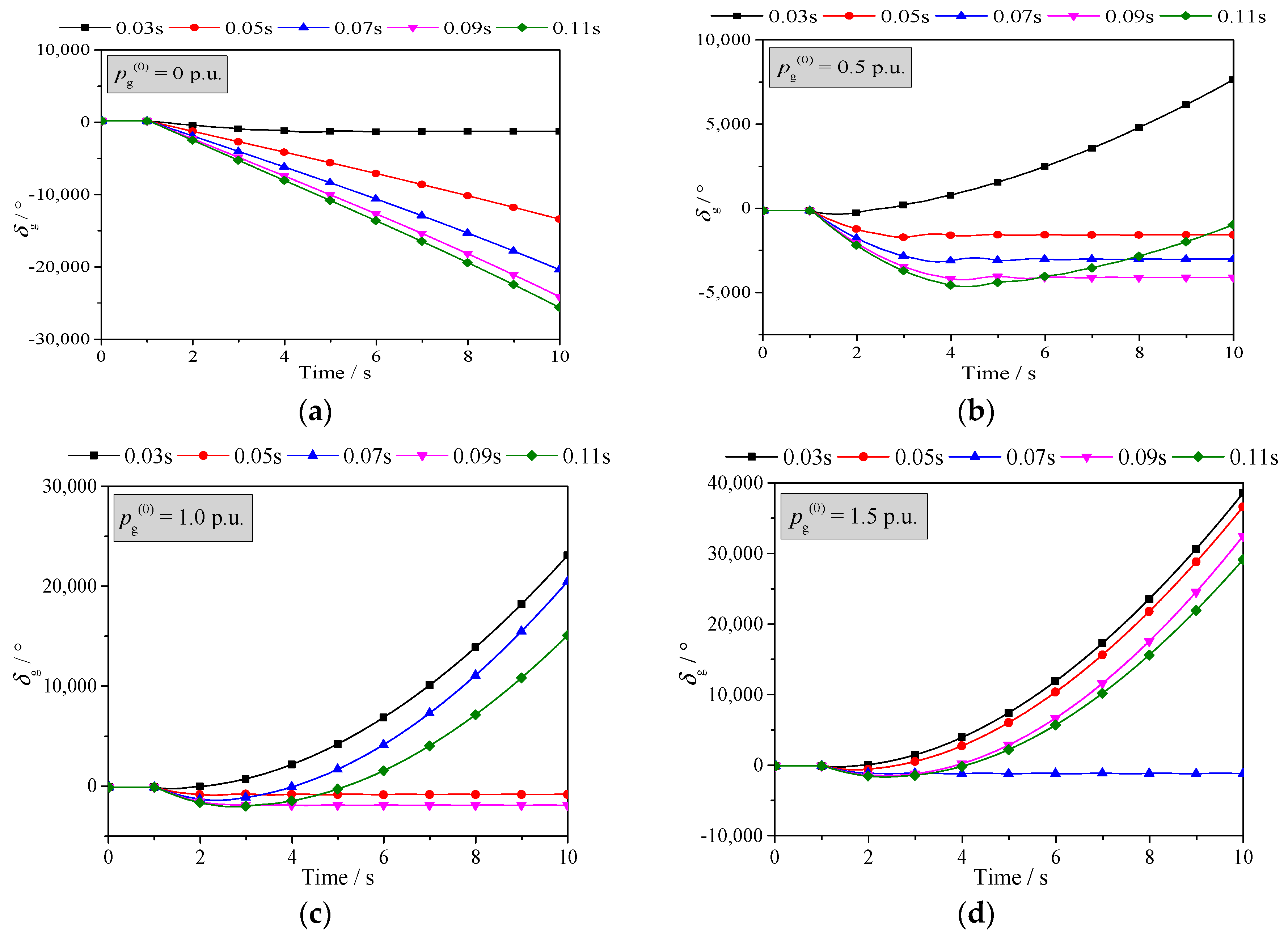
If a detailed generator model is adopted and the effect of the excitation system is considered (detailed data is given in the Appendix A.2), the results under the same fault are shown in Figure 12.

As shown in Figure 12, when p_g⁽⁰⁾ = 0 p.u., if the fault clearing time is 0.03 s, the system can keep stable; if the fault clearing time is 0.05 s, 0.07 s, 0.09 s, or 0.11 s, the system will lose stability. When p_g⁽⁰⁾ = 0.5 p.u., if the fault clearing time is 0.05 s, 0.07 s, or 0.09 s, the system can keep stable; if the fault clearing time is 0.03 s or 0.11 s, the system will lose stability. When p_g⁽⁰⁾ = 1.0 p.u., if fault clearing time is 0.05 s or 0.09 s, the system can keep stable; if fault clearing time is 0.03 s, 0.07 s, or 0.11 s, the system will lose stability. When p_g⁽⁰⁾ = 1.5 p.u., if fault clearing time is 0.07 s, the system can keep stable; otherwise, the system will lose stability.

When the system loses stability, if p_g⁽⁰⁾ = 0 p.u., δ_g will keep decreasing; if p_g⁽⁰⁾ is positive, δ_g will keep increasing after a certain time of decreasing. This is the same as the result of the classical model.

In conclusion, if a detailed generator model is adopted and the effect of the excitation system is considered, the stability of the system is uncertain, it depends on the value of the fault clearing time. However, the fault clearing time that keeps the system stable is segmented, so there is no fault critical clearing time.

9. Conclusions

On the conception of half wavelength power transmission, which was put forward in the 1940s, and is becoming a hot topic again, this paper makes an in-depth analysis with theoretical derivation and numerical calculation. The main conclusions are as follows:

(1)

There exists a resonant transmission distance in the half-wavelength transmission system. The resonant transmission distance is only related to the equivalent reactance of the sending end and the receiving end system, and is independent of the equivalent voltage source of the sending end and the receiving end system, and is less than the half wavelength.

(2)

Under the resonant transmission distance, the maximum voltage along the transmission line will reach infinity. Therefore, the transmission distance of the half-wavelength transmission system must be larger than that of the resonant transmission distance.

(3)

A transmission distance greater than the resonant distance is necessary for the small signal synchronization stability of the half-wavelength transmission system because when the transmission distance is less than the resonant transmission distance, the half-wavelength transmission system loses its small signal synchronization stability.

(4)

There exists a most serious fault location along the transmission line. When a three-phase short circuit fault occurs at this location, the most serious power-frequency overvoltage occurs at the point a quarter of wavelength from this location, and the value of the overvoltage is larger than 10 p.u.

(5)

When a three phase short circuit occurs at the most serious fault location, if the generator is modeled with the classical model and the damping is ignored, the system always loses its transient synchronization stability regardless of the fault clearing time and the initial transmission power.

(6)

When a three-phase short circuit occurs at the most serious fault location, if the generator is modeled with its detailed model and the effect of the field excitation and its control system is considered, the transient synchronization stability of the system is uncertain, i.e., the transient synchronization stability has no definite relationship with the fault clearing time and the initial transmission power.

(7)

Because the transient power frequency overvoltage of the half-wavelength transmission system exceeds 10 p.u. and the transient synchronization stability cannot be guaranteed, the conception of the half wavelength power transmission cannot be established, and the half wavelength transmission system is not feasible.