Pan-European Analysis on Power System Flexibility

Abstract

Ongoing deployments of intermittent non-synchronous power generators (i.e., wind turbines and photovoltaics) challenge power (electricity) system security in terms of matching power generation and demand. Higher flexibility in the future generation fleet and power demand are likely to play an essential role in maintaining secure operation of the power system. This paper proposes a stepwise methodology based on a set of indicators for future power system flexibility analysis through assessing (i) flexibility requirements, (ii) available flexibility resources, and (iii) power system adequacy. The proposed methodology is applied to a European case for 2020 and 2025 scenarios. The insights gained from this study can be used as input in distributing power balancing resources and to introduce new balancing products in a power market. Benefits of the integrated energy market are presented.

1. Introduction

The European power (electricity) system is currently subject to profound changes and so it will be during the next few years. On 30th November 2016, the European Commission published the new legislative package “Clean Energy For All Europeans”, designed with the aim of further completing the single internal market for electricity and implementing the Energy Union [1]. One of the key elements of this legislative proposal is the deepening of integration of the European power markets. It is important to develop new operational policies supporting power system evolution towards a more intermittent, non-synchronous generation fleet, while considering challenges to system stability and uncertainty from wind and solar generation. Thus, there is the need to study operational flexibility for managing large quantities of variable renewables when performing future electrical system analysis. Flexibility in this paper refers to the ability of a power system to ensure power balance (i.e., power generation equals demand at any time). This is challenging when deployment of generators from non-dispatchable Renewable Energy Sources (RES) is high.

When analyzing high RES scenarios, it is important to assess the flexibility requirements and availability from the generation fleet to design specific measures to cope with the uncovered needs. Some new elements are considered essential in the evolution of the system: a greater responsiveness of consumers (i.e., demand response), the deployment of energy storage facilities, and an efficient use of existing and planned cross-border power exchange capacities.

There is extensive work on power system flexibility. Recent reviews can be found in [2,3,4]. Some work focuses on qualitative analysis or theoretical developments [4]. Setting up a quantitative flexibility evaluation method is essential to identify flexibility needs and sources; however, there is no consensus on which metrics are best suited [5], and how the indicators relate with RES curtailment or loss of load. Moreover, there is the need to find a compromise between computational complexity and meaningfulness of the indicators [6].

From the methodological point of view, there are four sequential steps to assess flexibility according to [7]:

• Flexibility requirements;
• Availability of flexibility resources;
• Power system adequacy;
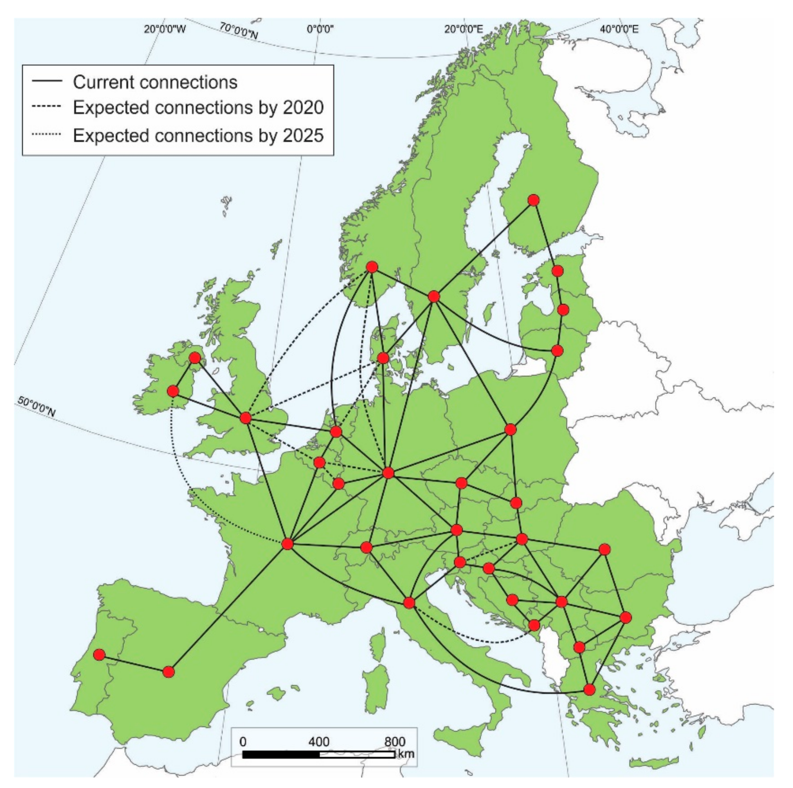
• Power transmission grid adequacy.

Each step covers different aspects of the flexibility assessment, completes collected information from the previous steps and is characterized by an increasing level of complexity and data requirements

Under Step 1—flexibility requirements—the dynamics of the net load, magnitude of ramps, frequency of occurrence, and timing are perceived over a variety of time horizons. Net or residual load is defined as the difference between electricity demand and the amount supplied by non-dispatchable renewables. This is a deterministic assessment aiming at evaluating the flexibility needs of the electricity system under the assumption that no renewable curtailment is permitted.

Under Step 2—available flexible resources—the existing flexibility resources in the power system are identified. The goal of this level is to understand the potential flexible capabilities in a given system. Like Step 1, this is a deterministic analysis. The technical specificities of the flexibility resources are not examined in full detail, neither the impact of other factors such as market and operational arrangements.

The system flexibility analysis, step 3, includes the assessment of the power system adequacy once flexibility resources have been dispatched, in comparison with the flexibility required by the system at different times. Here, a chronological power system modeling for one year with a 1-h time step is applied. This analysis can have various degrees of complexity and detail: from a deterministic analysis in which only the specific technical constraints of the generating units are considered, to a probabilistic one where RES and load variability are taken into account based on historical data and Monte-Carlo simulations. Moreover, the full spectrum of flexibility resources such as demand response or RES curtailment, can be systematically included, as well as market and operational arrangements (e.g., reserve capacity constraints of the system).

Finally, step 4 is built on step 3 analysis to include the constraints of the power transmission network such as thermal limits of the transmission lines when distributing power flows. The objective is to determine the extent to which the transmission network impacts the ability of the system operator to balance the system using the available flexibility resources. This final step is out of the scope of the present work given that would require detailed modelling of the transmission network in the examined area (Europe).

Summarizing, in step 1, a mapping of the future needs in power system flexibility is performed. In step 2, a systematic recording of the flexibility resources is conducted. The combination of these two steps can provide useful insights to both power system operators and policy makers. However, the ability of the system to cope with the flexibility challenges is investigated in steps 3 and 4. Thus, the value of flexibility resources can be fully analyzed, while assessing the impact of policy, market, technical and operational arrangements, such as reserve dimensioning, planned and unplanned outages, transmission congestions and active participation of demand response and RES into markets.

The main element to consider in flexibility analysis is the more frequent and extensive need of ramping capabilities. There is already extensive work performed on ramp analysis: two regional transmission system operators in the United States, California Independent System Operator (CAISO) and Midcontinent Independent System Operator (MISO), have proposed market-based flexible ramping products to avoid balance violations caused mainly by the variability and uncertainty in generation from RES [8]. The first step needed when designing new market products is the assessment of the requirements of the system. Ramp events should be characterized in terms of ramping start and end time, ramping duration, ramping rate, and ramping magnitude [9]. Not only deeper ramp events will be a constant new feature in the future system, but also inertia will be challenged. The phase-out of coal and nuclear power plants, at least in some European countries, and the significant increase of wind and solar generation will transform the system towards an inverter-dominated grid [10].

The objective of this work is to propose a methodological approach to analyze power system flexibility in a systematic way. The focus is in the evolution of the European power system from 2020 to 2025, where the new legislative proposal will enter into force. There are several previous works on specific countries, as Germany [11], France [5] and Greece [12], but less on assessing the European system as a whole [13]. Although there are several previous works focusing on the analysis of 1-h ramps, we consider essential to extend this analysis up to 3 or 4 hour ramps, at least in countries with significant solar photovoltaic (PV) installed capacity, as these longer-lasting ramps impact the operation of the grid and the sizing of the operational reserve needs. A more complete analysis considering the evolution of system inertia is also included.

The insights gained applying the proposed methodology can then be used as input to guide the development of new flexibility resources and to design new market products.

The following in this article is organized as follows: Section 2 proposes the metrics for the first three power system flexibility assessment steps conducted in this work; Section 3 presents the European power dispatch model. Section 4 shows the main results of the flexibility analysis. Finally, Section 5 highlights the main conclusions.

2. Power System Flexibility Assessment

In this work, each step of the flexibility analysis was performed considering a set of indicators. This allowed comparison between countries and between analyzed years (2020 and 2025).

2.1. Step 1: Flexibility Requirements Indicators

The main topic was ramp analysis over a variety of time horizons: magnitude of ramps, frequency of occurrence and timing. Net (residual) load is the demand that must be supplied by dispatchable resources, mainly the conventional generation fleet, but also the storage and demand response, if all of the renewable energy is to be utilized [14].

Reference [15] provides a wide range of indicators to cover this analysis related to renewable energy penetration into the power system:

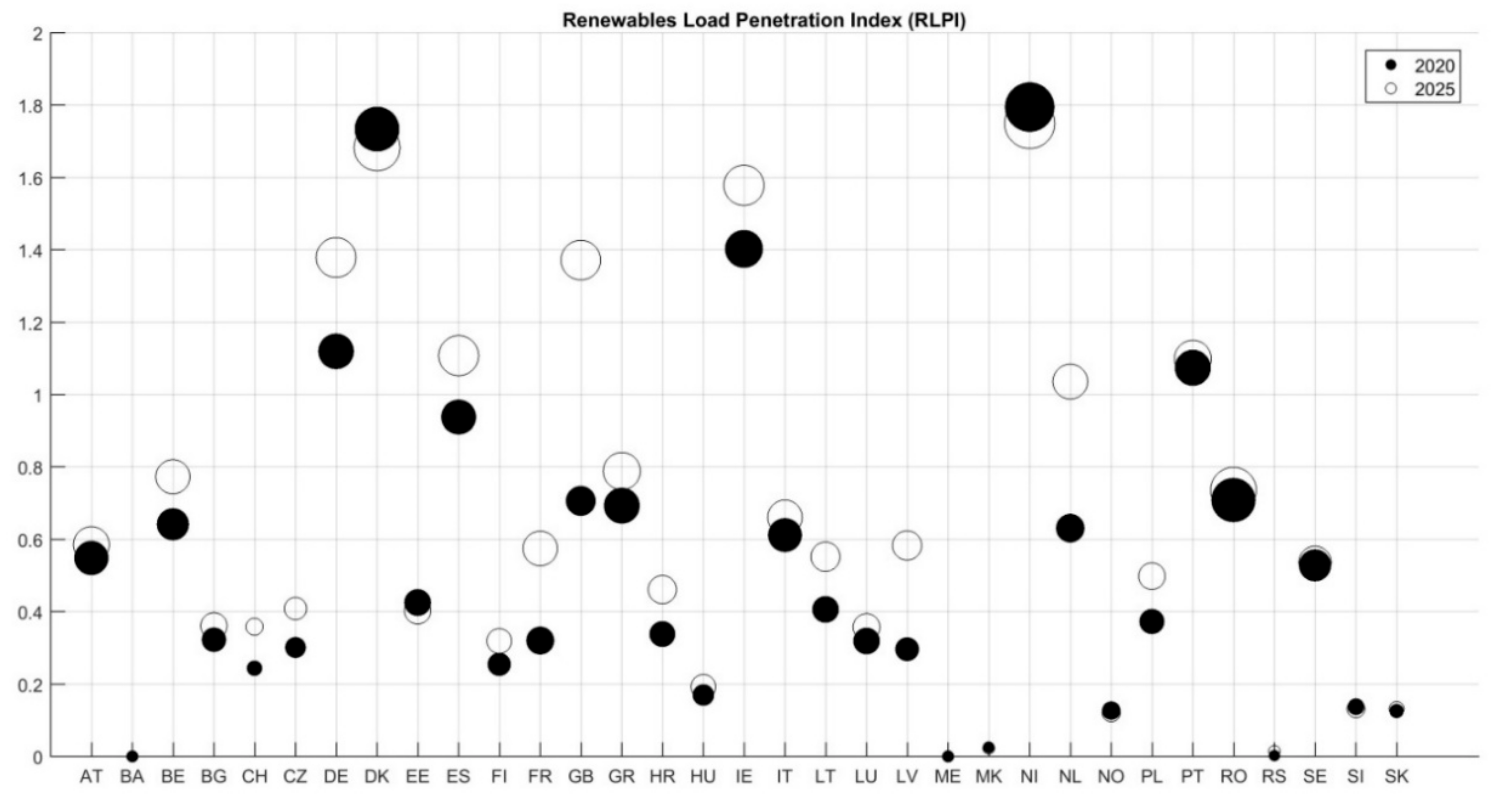
• RES Load Penetration Index (RLPI). This is the maximum hourly coverage of load by non-dispatchable renewables energy generation (wind and solar):

  $$RLPI\left(t\right)=\max \left(\frac{W\left(t\right)+S\left(t\right)}{L\left(t\right)}\right)\mathrm{for}t=1,2,3,\dots ,8760$$

  (1)

  where W(t), S(t), and L(t) are wind and solar energy generation, and the demand at time t respectively.
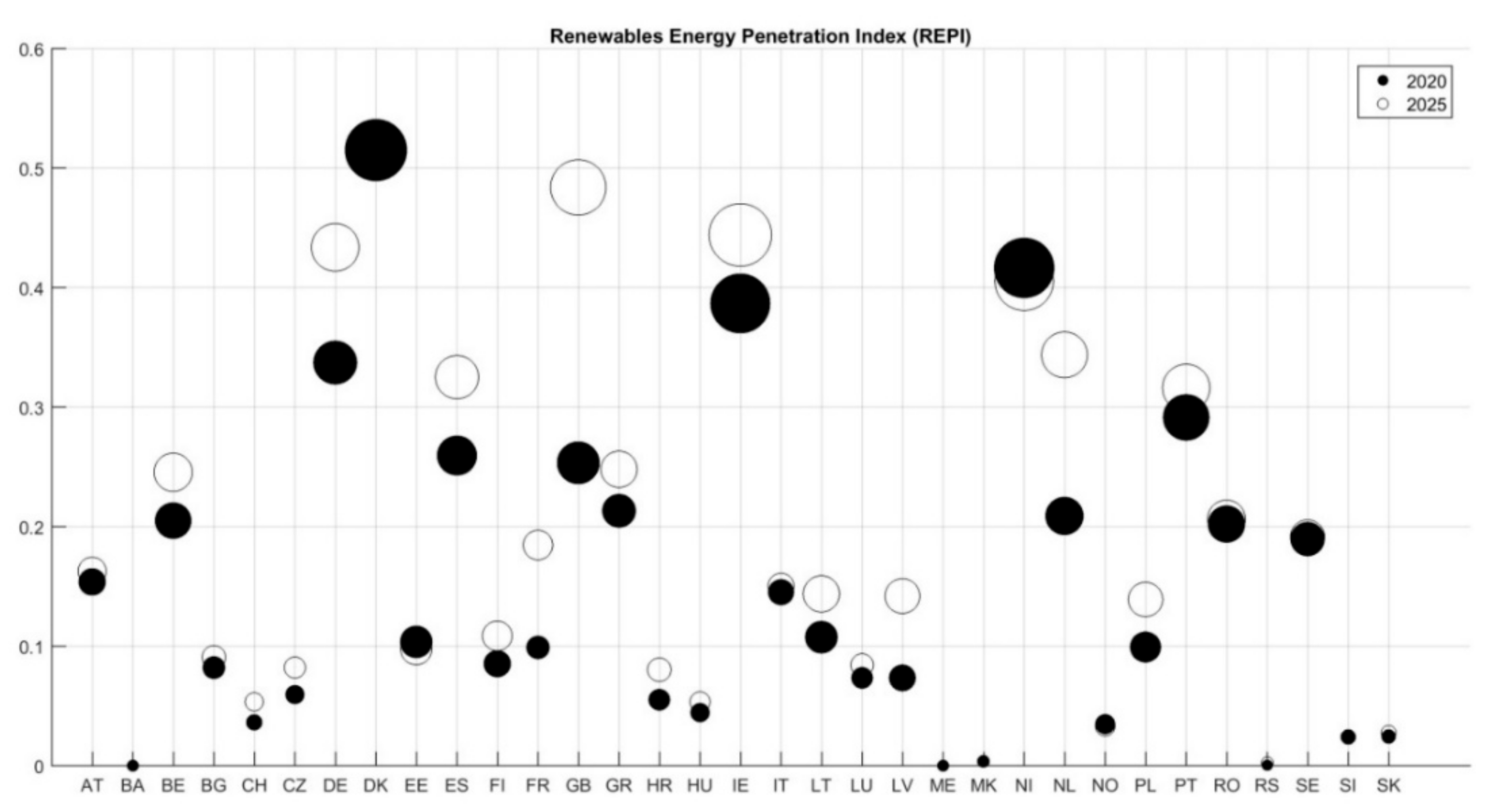
• Renewable Energy Penetration Index (REPI). This is the average value of demand covered by wind and solar generation:

  $$REPI= \frac{W_{annual}+S_{annual}}{E_{annual}}= \frac{{{\displaystyle \sum }}_{t=1}^{8760}W\left(t\right)+S\left(t\right)}{{{\displaystyle \sum }}_{t=1}^{8760}L\left(t\right)},$$

  (2)
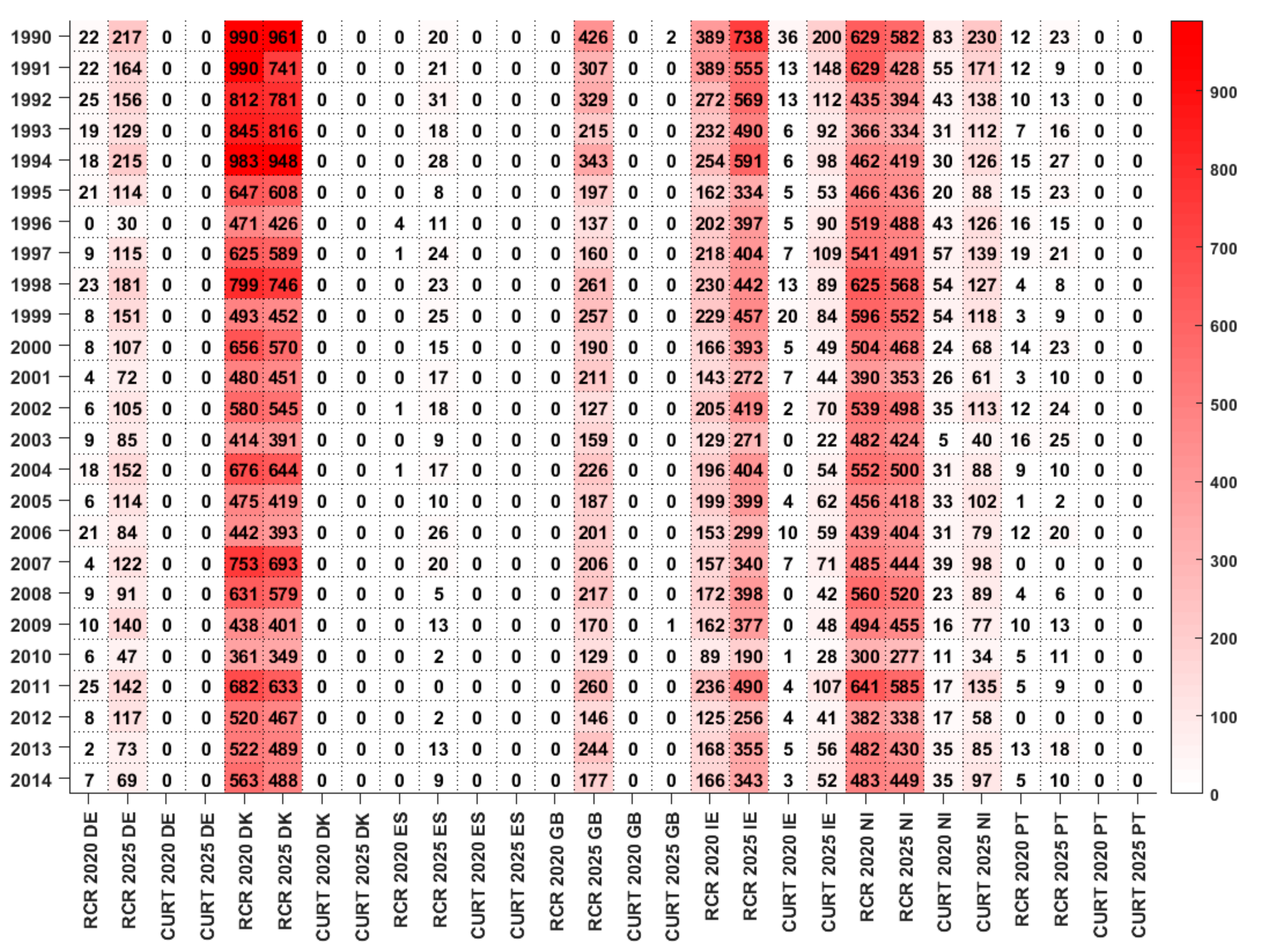
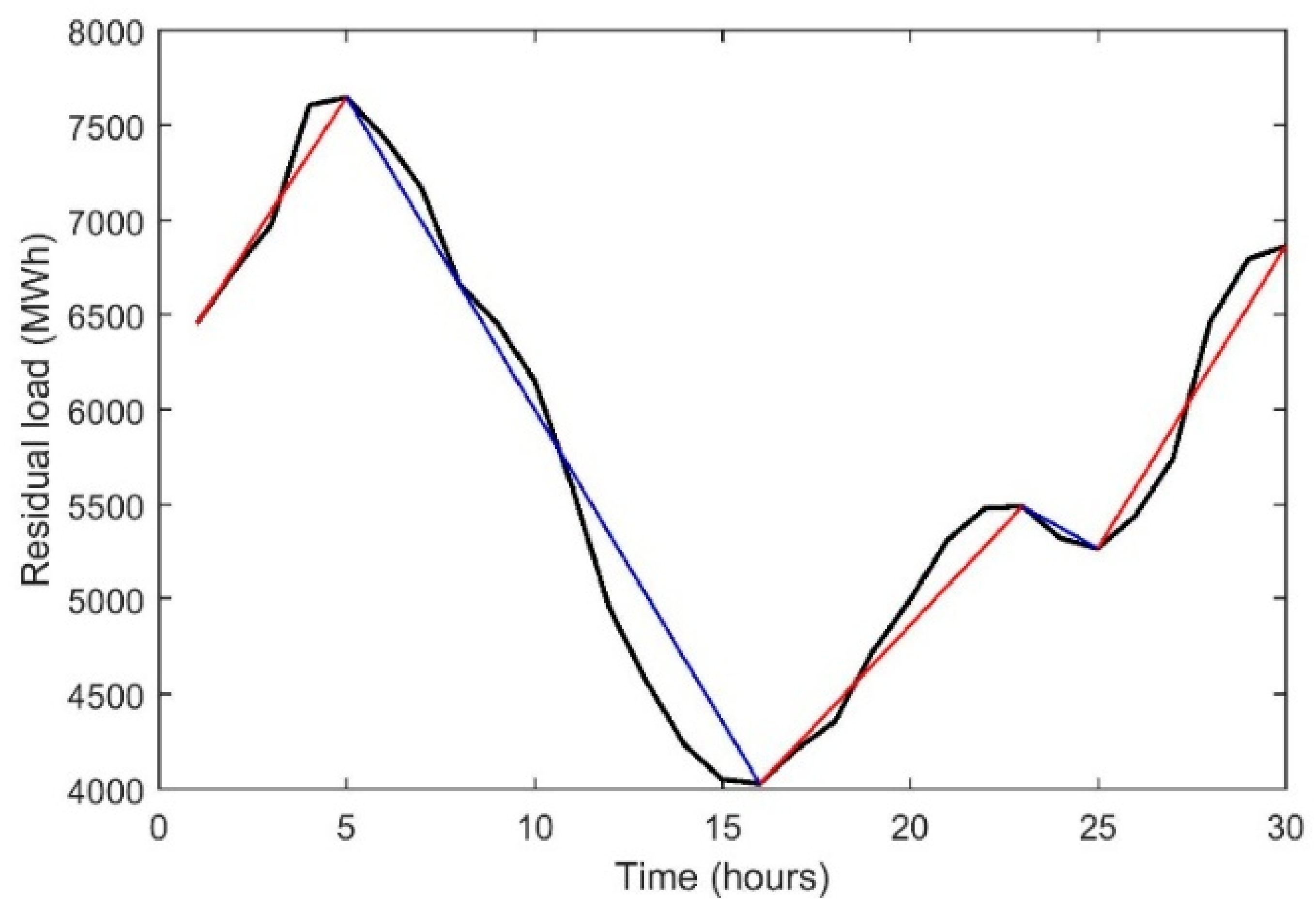
• Renewable energy generation Curtailment Risk (RCR):

  $$RCR= \frac{number of hours in the year with RL\left(t\right) < 0}{8760},$$

  (3)

  where RL(t) is the residual load at hour t. In this work, the residual load is defined as follows:

  $$RL\left(t\right)= L\left(t\right)-W\left(t\right)-S\left(t\right).$$

  (4)

Other definitions can be found in the literature, but were kept as simple as possible to gain insights into the impact of wind and solar generation on the power system.

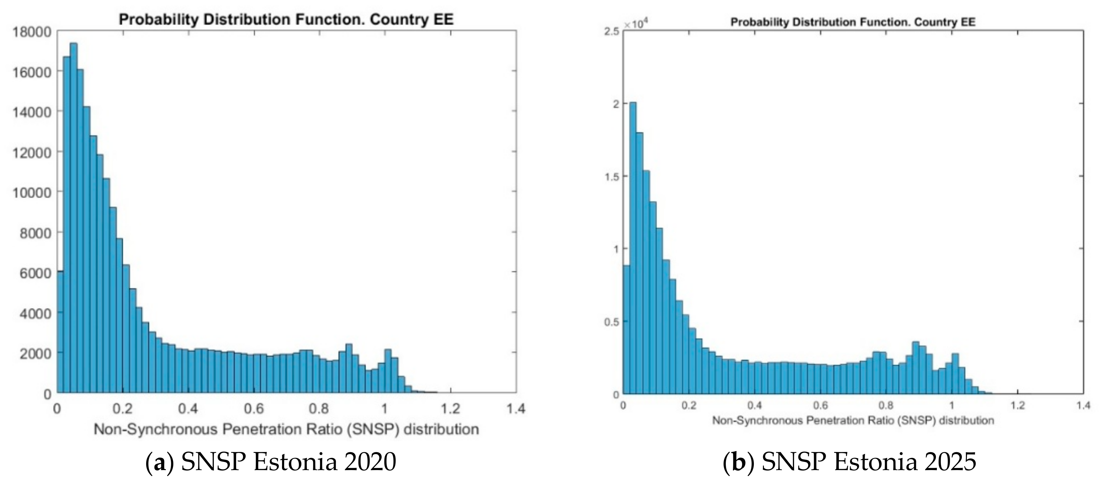
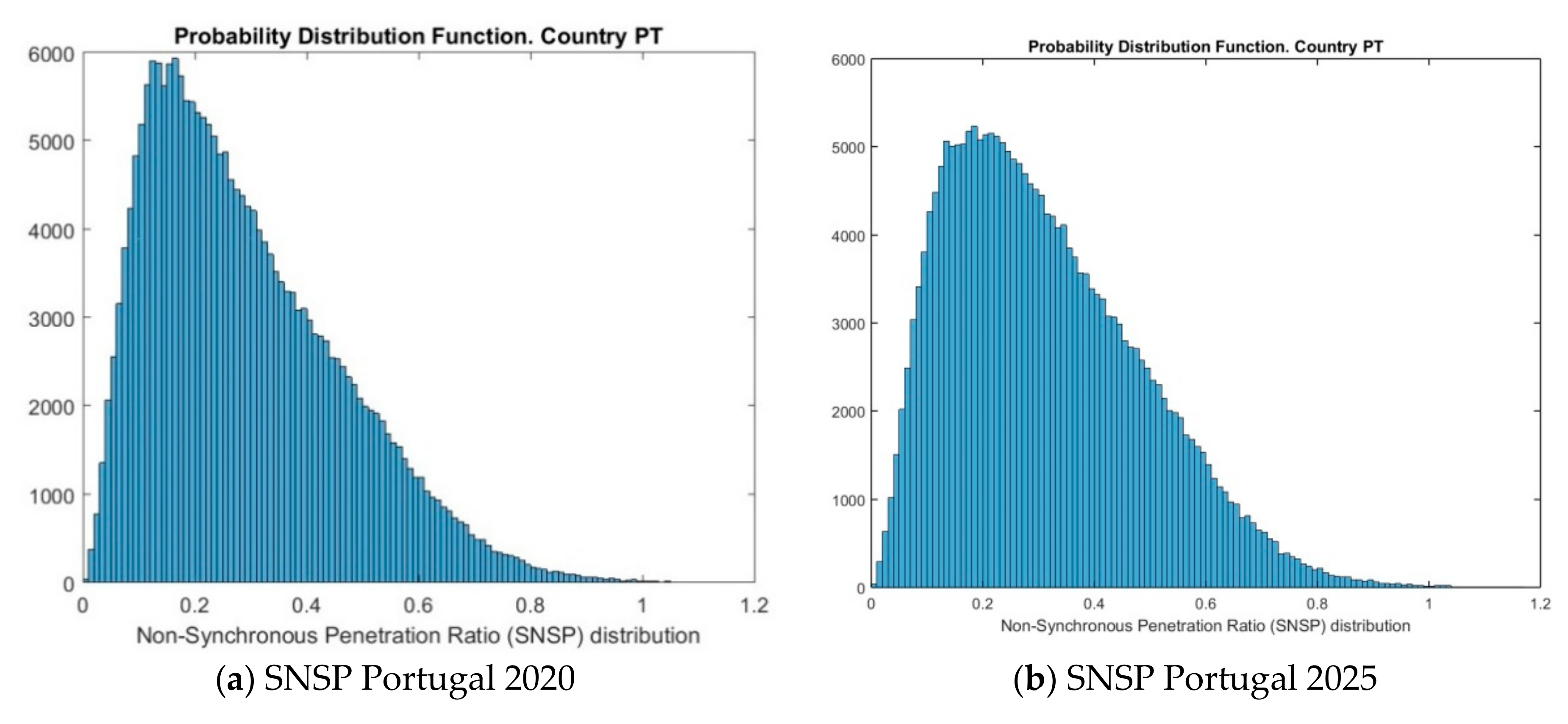
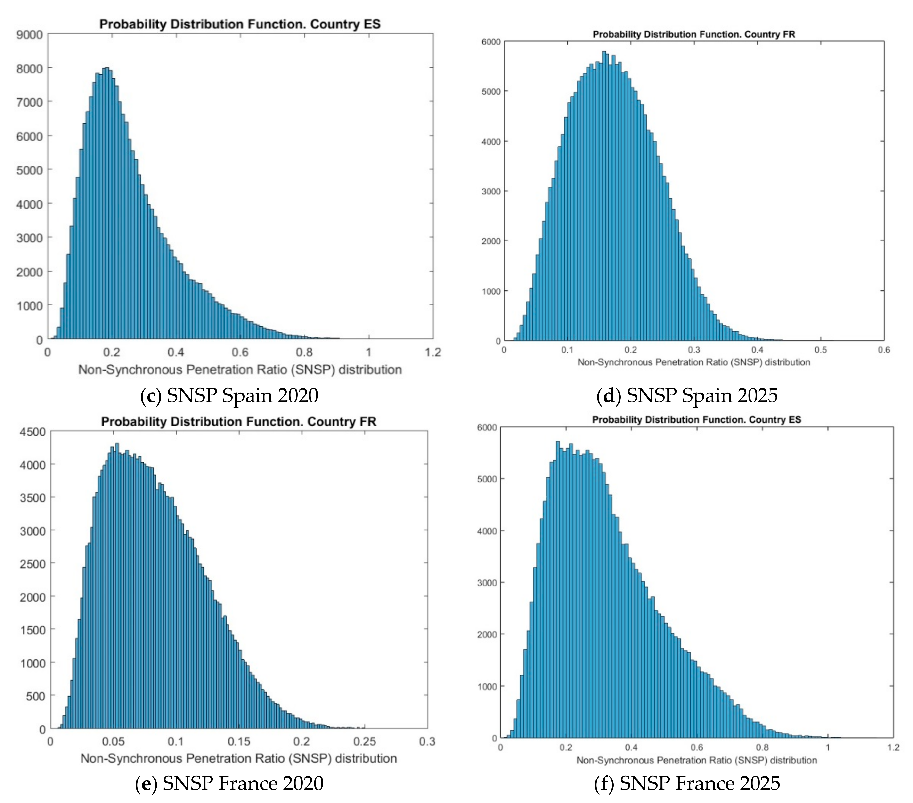
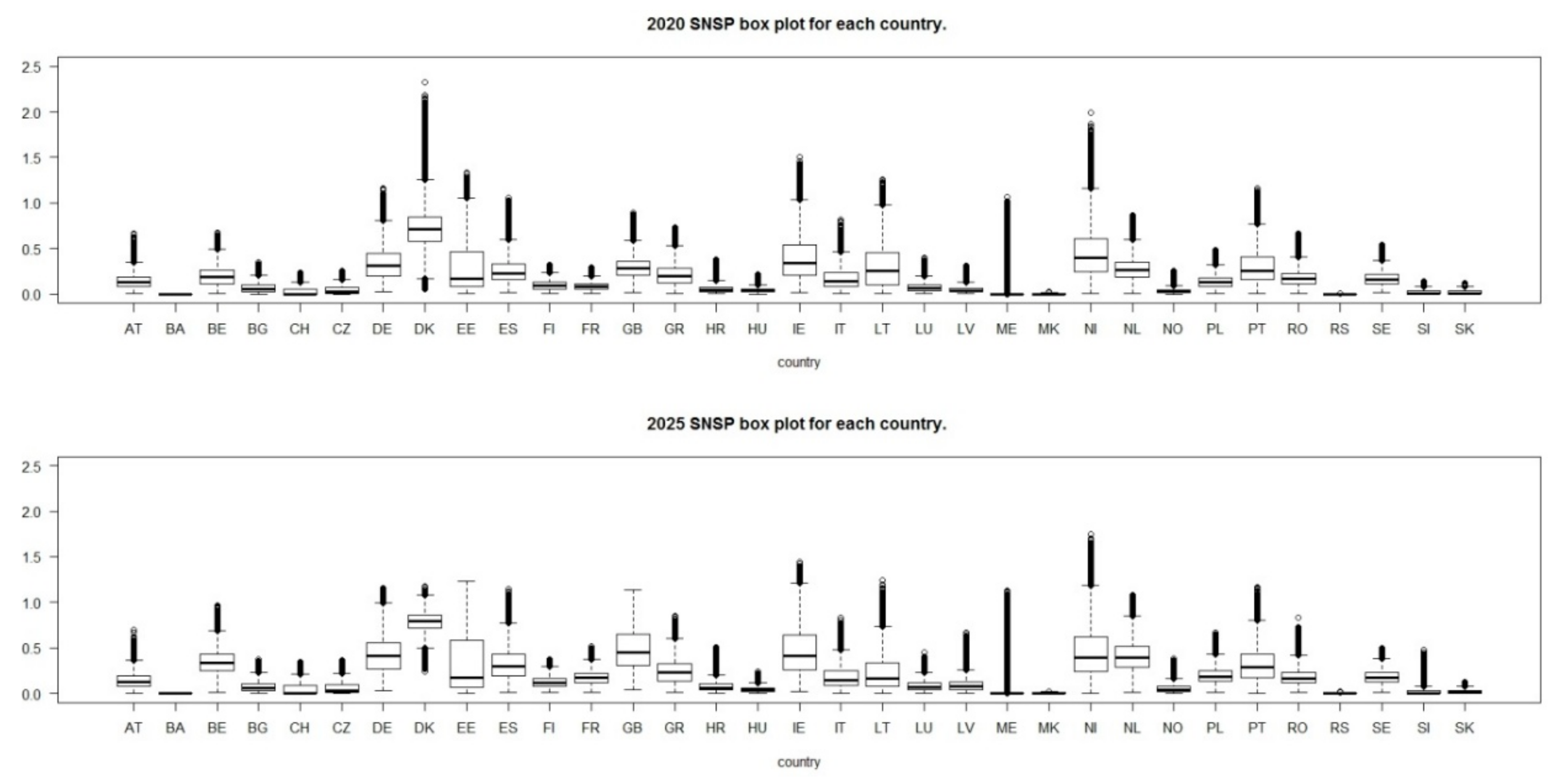
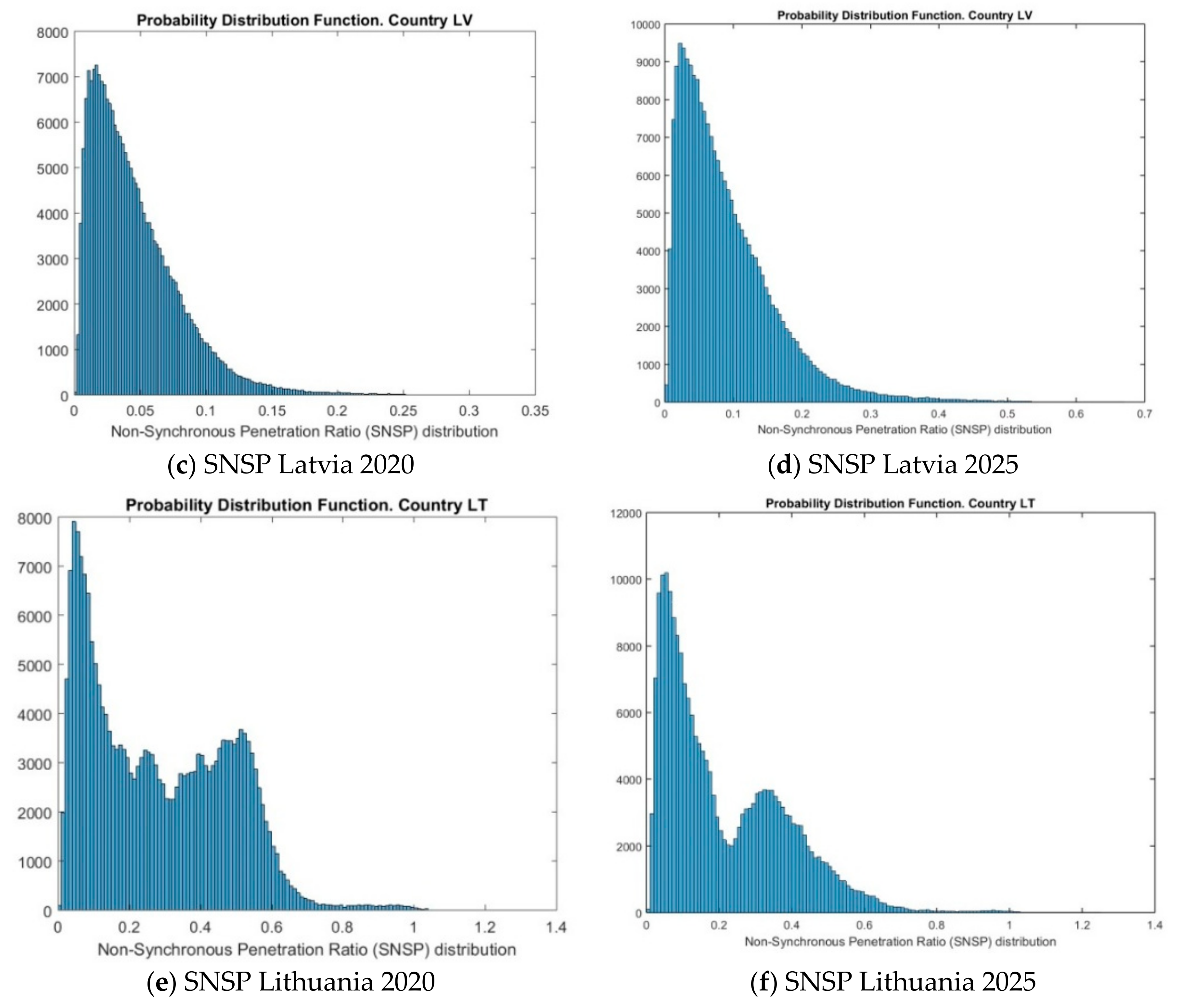
• Non-Synchronous Penetration Ratio (SNSP). An additional concern through the transition to a low carbon system is the evolution of system inertia, which is an important element of frequency stability. In [16], the authors propose the following indicator to monitor the evolution of the system inertia:

  $$SNSP\left(t\right)= \frac{W\left(t\right)+HVDC{\left(t\right)}_{import}}{L\left(t\right)+HVDC{\left(t\right)}_{export}},$$

  where W(t) refers to wind power generation, L(t) is the system demand, and HVDC(t)_import and HVDC(t)_export are the imported and exported power through high voltage direct current (HVDC) interconnections respectively, all of them at time step t. This metric can be generalized as follows:

  $$SNSP\left(t\right)= \frac{{{\displaystyle \sum }}^{}P{\left(t\right)}_{i{n}_{inverter}}}{{{\displaystyle \sum }}^{}P{\left(t\right)}_{out}}= \frac{W\left(t\right)+PV\left(t\right)+HVDC{\left(t\right)}_{import}}{L\left(t\right)+ P{\left(t\right)}_{export}}.$$

  (5)

  Notice that the denominator HVDC(t)_export has been replaced by P(t)_export. This is because the original work [16] was focused on Ireland, which has only one interconnector, which has HVDC technology. It is worth to say that inverters can emulate system inertia, so when this capability is implemented, the numerator can be reduced accordingly (the emulation is different depending on the system the inverter is connected to: wind, PV, or HVDC interconnection). For example, since 2006, Hydro Quebec Transénergie has required system inertia emulation to wind farms with rated output greater than 10 MW [17].

2.2. Step 2: Flexibility Resources Indicators

The objective of this step was to identify the potential flexible resources that exist in the system. The proposed indicators were the following:

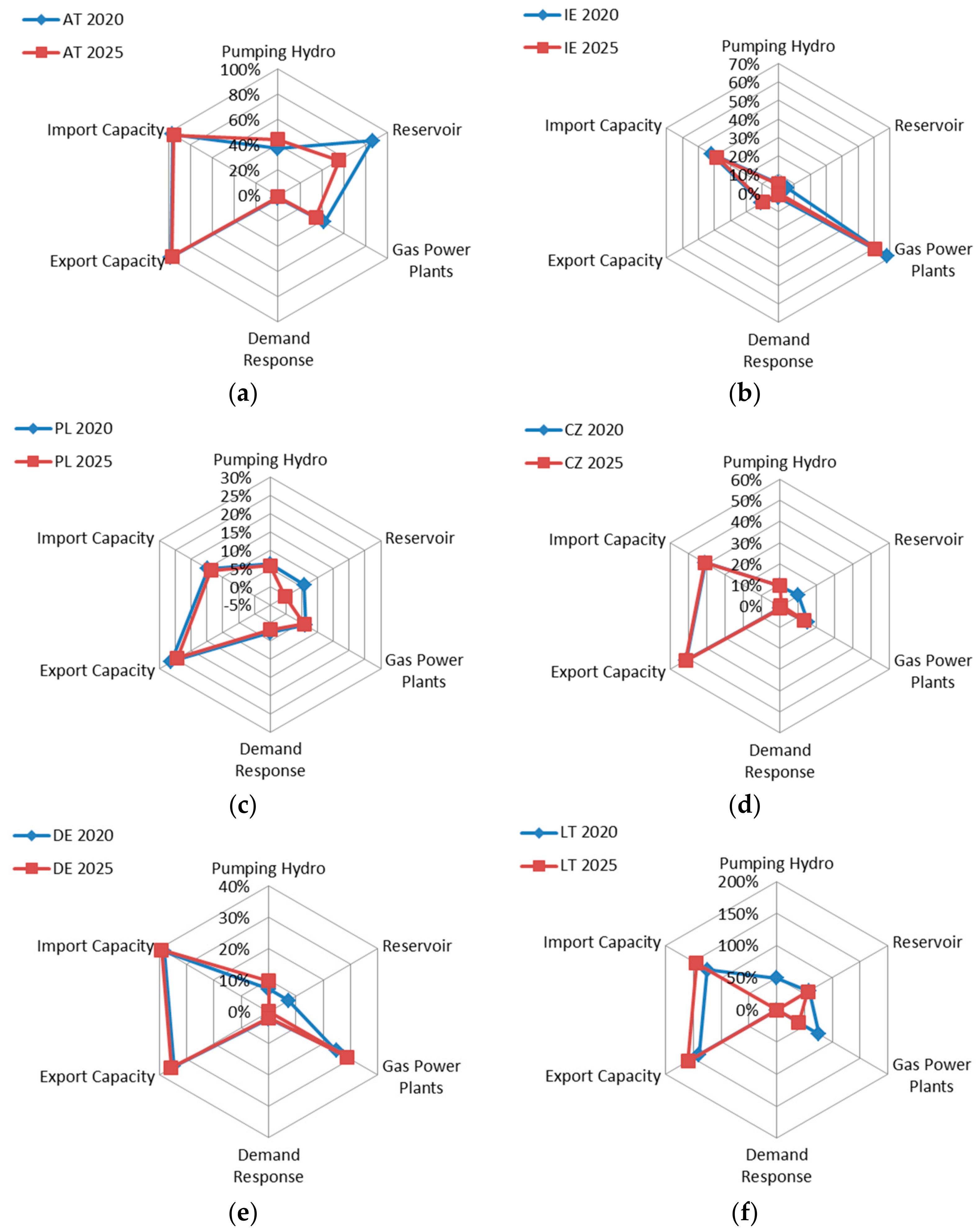
• Flexible Capacity Ratio (FCR): the percentage of installed capacity of a resource type relative to peak demand. This metric can be used to evaluate the diversity and potential capability of flexibility sources through a “flexibility chart” that is employed to visualize the dominant factors and compare the variety of solutions in different countries/areas [18].

Another way to assess the endowment of flexibility resources of a system is provided by the GIVAR visual tool [19] in which power area size, grid strength, interconnection, number of power markets, and flexibility of dispatchable generation portfolio serve as proxies for flexibility. The GIVAR tool presents a broader range of power system properties and types of measurement, such as the dispatchability of the portfolio, and can include capacity, and assumptions about fuel supply and specific analyses of cycling capabilities.

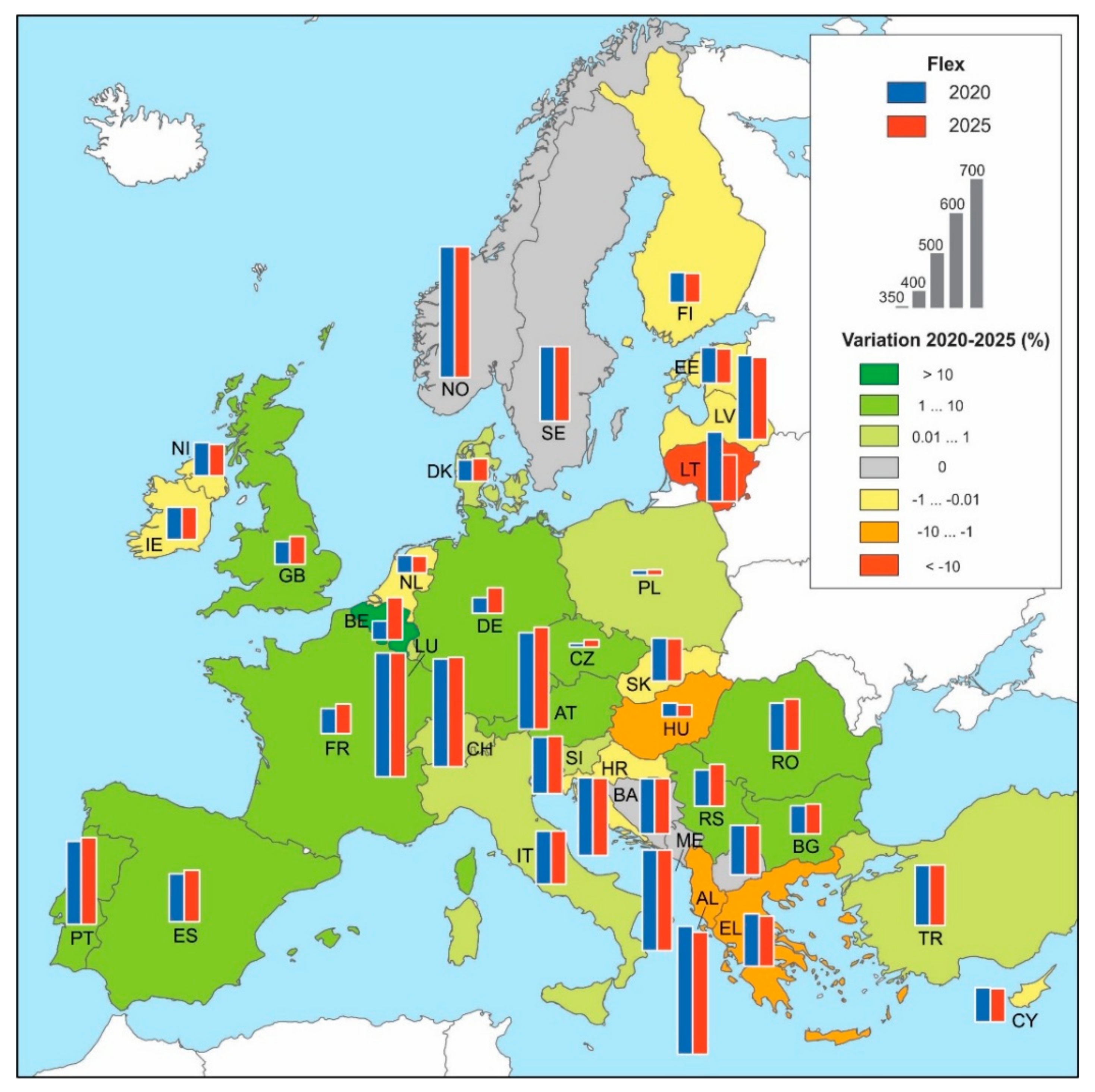
• Flexibility index for a power system [20]:

  $$FLE{X}_A= {{\displaystyle \sum }}_{i\in A}\frac{P_{\max \left(i\right)}}{{{\displaystyle \sum }}_{i\in A}{P}_{\max \left(i\right)}}flex\left(i\right),$$

  where $P_{\max }\left(i\right)$ is the maximum capacity of generator i and flex(i) is the flexibility index for generation unit i, which is defined as follows:

  $$flex\left(i\right)=\frac{\frac{1}{2}\left[P_{max}\left(i\right)-P_{min}\left(i\right)\right]+\frac{1}{2}\left[Ramp\left(i\right)\right]}{P_{max}\left(i\right)},$$

  (6)

  where $P_{max}\left(i\right) and P_{min}\left(i\right)$ are the maximum and minimum stable generation capacity of generator i respectively. $Ramp\left(i\right)$ is the average value of $Ram{p}_{up}\left(i\right) and Ram{p}_{down}\left(i\right)$, which indicates the speed of a unit to change its position within its operating range [$P_{max}\left(i\right)- P_{min}\left(i\right)$]. For comparison purposes the index was normalized by dividing by the maximum capacity. This indicator only assessed the flexibility of the generation fleet but not the flexibility due to other means, although it can be generalized using the same formula.

2.3. Step 3: Adequacy Indicators

Inflexibility indicators were the main tool to document the deficits in flexibility [14]. Signs of inflexibility include:

• Renewable energy curtailments.
• Frequency excursions or dropped load (energy not served, ENS). Additional indicators to complement ENS are the loss of load duration (LLD) and loss of load occurrence (LLO).
• Area balance violations which are deviations from the schedule of the area power balance.
• In the wholesale power market, negative market prices and price volatility.

3. Model and Data

Step 3—power system adequacy—was assessed with a Europe-wide power system model. The model is developed for 2020 and 2025 scenarios following the European Network of Transmission System Operators (ENTSO-E) Mid-term Adequacy Forecast (MAF) 2016 [21]. The model [22] comprises of (i) 32 European countries (Austria, Belgium, Bosnia and Herzegovina, Bulgaria, Croatia, Czech Republic, Denmark, Estonia, Finland, France, Former Yugoslav Republic of Macedonia, Germany, United Kingdom (which is modelled as two different regions: Great Britain and Northern Ireland), Greece, Hungary, Ireland, Italy, Latvia, Lithuania, Luxembourg, Montenegro, Netherlands, Norway, Poland, Portugal, Romania, Serbia, Slovakia, Slovenia, Spain, Sweden, and Switzerland, modelled as 33 nodes), and (ii) the cross-border transmission connections between these nodes. The modelled nodes and their cross-border connections are shown in Figure 1.

The model was built on the PLEXOS^® power market simulation software [23]. A time series modelling approach is applied: each scenario is a one-year period with an hourly time step, using deterministic programming techniques that aim to minimize an objective function (the total cost), subject to some constraints representing the physical characteristics of the system: power balance, power plant availability, power reserves, power transmission constraints, and fuel/emissions prices, up and down ramping capabilities of the generation fleet, etc. Thorough description of the model is available in a previous study [14], which includes objective function of the optimal dispatch of power generators, power system constraints, and details on input data.

Generation and cross-border capacities, hourly demand profiles, and CO₂ prices for 2020 and 2025 modelling scenarios were set following the modelling dataset of the MAF 2016 published by ENTSO-E [21].

Wind and solar hourly generation profiles are acquired from an open database—http://renewables.ninja/ version 1.0 [24,25] based on historical records covering 25 years—1990–2014. Every future scenario year (e.g., 2020/25) was modelled under 25 different historical weather conditions. Monthly water inflow profiles for the hydro power plants was extracted from the historical generation records of Eurostat [26].

The main properties and constraints of the modelled generation technologies followed the Joint Research Centre report on projected energy technology indicators [27]. Outage rates for power generators were obtained from the World Energy Council [28]. The unplanned outages were distributed randomly through a year; but the planned outages were modelled to occur mostly during times of low electricity demand. Outage pattern was different from one historical year to another.

4. Results and Discussion

4.1. Step 1: Flexibility Requirements

Four main indicators have been estimated considering 25 different renewable energy generation profiles: RLPI, REPI, RCR and SNSP represented from Figure 2, Figure 3, Figure 4 and Figure 5 respectively.

Figure 2 represents the RLPI, whereas Figure 3 represents REPI, which is the average fraction of demand covered by wind and solar along the year. It is important to highlight the different scale of the two indicators: for example, in the case of Denmark, the average REPI value is 0.52 whereas the average RLPI is 1.73, that is to say, more than three times larger. REPI represents the average value of RES penetration and RLPI its maximum instantaneous value. Every time that RLPI is larger than 1 means that there is a surplus of variable RES generated energy. The installed capacity of wind and solar increases from 2020 to 2025 except for Estonia, Montenegro, Northern Ireland, and Norway, which remained constant. Yet, in these nodes, the demand increases, which is reflected in the lower RLPI and REPI values for 2025 than for 2020.

The nodes with the larger wind resource (i.e., equivalent generation hours) are Great Britain, Sweden, Ireland, and Finland while the nodes with the largest REPI are Denmark, Great Britain, Ireland, and Northern Ireland. The equivalent generation hours is defined as the ratio between the annual wind generation and the wind installed capacity.

Figure 4 shows the renewable energy generation curtailment risk indicator, RCR, for countries with a non-zero value for year 2020 and 2025. It represents the number of hours per year where the RLPI is larger than 1. RCR reflects the potential number of hours when there is a high risk of curtailment due to negative residual loads (i.e., renewable generation larger that demand).

Figure 5 represents the System's Non Synchronous Penetration (SNSP) ratio. To capture the main statistical characteristics of this indicator, the figure shows the boxplot for each node. With this type of graph, the shape of the distribution (whether it is symmetric or not), its central value, and its variability can be visualized easily [29]. It was observed that instantaneous values could be very high (more than 2.0 for the specific case of Denmark), which implies that some countries will depend on neighboring countries for dynamic stability. Share of reserves and balancing markets linked with an optimal use of interconnectors will be essential in the next future of the European power system, possibly along with provision of emulated inertia by large RES plants and modern HVDC interconnectors, to accommodate larger in-feeds through inverters.

Moreover, Figure A1 and Figure A2 in Appendix A represent the SNSP probability distribution function for some particular countries for the years 2020 and 2025. It can be seen that the shape of the distribution was not homogenous, and it depends mainly on the country (amount of imports and HVDC interconnector capacity and RES generation percentages). They clearly showed, in any case, a long right-hand tail which means that there would be periods with reduced value of inertia (associated with high RES production or high imports through HVDC interconnectors). Hence, frequency regulation is expected to become more demanding in the future.

Regarding ramp analysis, ramps are characterized by their start and end time, duration (or span), and magnitude. Although they are very well known and quasi-deterministic for demand and PV, the same does not hold for wind energy and as a consequence, for residual load. One of the main concerns is to know if the future conventional generation fleet can cope with the extreme variations of the residual load or additional tools are needed in the system (an increase in storage capacity, the deployment of demand response, pro-active curtailment of RES, etc.). Figure 6 shows how ramps are computed: every interval where the signal (residual load or wind energy) increases monotonically is considered as one up-ramp event (red line in the figure), and if it decreases it is considered a down-ramp event. This is important to analyses in order to dimension properly all the frequency reserve needs.

Table 1. Wind and residual load ramps. 2025. The maximum ramp span is the duration of the maximum ramp (which is the ramp with the largest magnitude). Span maximum rate is the duration of the ramp with the maximum average rate. Source: own elaboration.

	Wind Ramps					Residual Load Ramps
	Most Frequent Ramp Span (h)	Maximum Ramp (MW)	Maximum Ramp Span (h)	Maximum Average Rate (MW/h)	Maximum Average Rate Ramp Span (h)	Most Frequent Ramp Span (h)	Maximum Ramp (MW)	Maximum Ramp Span (h)	Maximum Average Rate (MW/h)	Maximum Average Rate Ramp Span (h)
AT	2	3514	26	2395	1	5	6292	16	2027	1
BE	2	4768	15	3548	1	5	7763	11	2943	1
BG	2	865	18	387	1	1	2917	10	514	1
CZ	2	661	20	311	1	4	3425	9	776	3
DE	2	51,834	27	25,626	1	6	67,086	19	30074	1
DK	1	5300	29	3558	1	1	6548	10	3602	1
EE	2	336	39	171	1	1	827	14	282	1
ES	2	23,360	25	11,616	1	6	31,224	18	17273	1
FI	2	2753	35	2040	1	1	4434	16	1973	1
FR	2	19,883	15	15,574	1	2	37,564	10	12,594	1
GB	2	36,624	37	20,622	1	5	50,288	16	26,593	1
GR	2	2883	17	1870	1	1	5964	16	1918	1
HR	1	783	30	187	1	1	2050	9	330	2
HU	2	738	27	516	1	1	2922	13	711	1
IE	1	3892	25	2768	1	1	6005	14	2373	1
IT	1	10,025	20	5830	1	5	34,739	17	5926	1
LT	2	578	35	370	1	1	1238	11	436	1
LU	2	161	14	134	1	1	475	10	184	1
LV	2	408	36	209	1	1	958	11	219	1
NI	2	1189	17	952	1	1	1884	12	936	1
NL	2	9677	27	5886	1	1	15,569	12	5844	1
NO	1	1218	20	932	1	1	7559	9	1346	4
PL	2	7085	35	4493	1	1	14,582	13	5386	1
PT	1	4913	21	3962	1	1	7287	14	3133	1
RO	2	3678	31	2600	1	1	5327	10	3311	1
SE	2	6299	28	5829	1	1	10,471	11	5227	1
SI	1	40	13	20	1	1	1105	9	218	4
SK	2	95	25	52	1	1	1461	6	398	1

shows the main characteristics of wind and residual load ramps for 2025 obtained with the 25 historical meteorological years. We analyzed three different characteristics: (i) most frequent ramps; (ii) maximum ramps in respect to their absolute magnitude as well as their respective span (i.e., duration); and (iii) maximum ramp-rates along with their span. Comparing the two of them, it can be observed that most frequent wind ramps were usually two-hour ramps, although for the residual load, two different country sets were distinguished: one with 1-h ramps, and others with 4-, 5-, or 6-h ramps as the most frequent. Residual load maximum ramps were always larger than wind maximum ramps. For rates, wind ramps maximum rates were smaller than residual load maximum rates for most of the nodes (except Austria, Belgium, France, Ireland, Northern Ireland, the Netherlands, Portugal and Sweden). The maximum rate for ramp duration is always one hour for wind, but this is not the case for residual load, which can be up to 4 h.

Figure 7 represents 1-h to 3-h residual load ramps histograms for Austria and Italy. It can be seen that negative and positive ramps were not symmetric, so ramp-up and ramp-down requirements were different too. Depending on the ramp span, its characteristics varied: for example, in the case of Austria, positive 1-h ramps were more frequent and larger than the negative ones. On the other hand, negative 3-h ramps were more frequent and larger than the positive ones. It is necessary to differentiate and study ramps specifically, considering its sign and length, if new ramping products are to be introduced in the market.

4.2. Step 2: Flexibility Resources

Having regard to the system requirements, the second stage is to assess the potential capabilities of the resources. Figure 8 represents the evolution of the Flexible Capacity Ratio (FCR) from 2020 to 2025 for six different countries. As we have shown in the previous section the asymmetry of the ramping requirements, the import capacity (for ramping-up requirements) and the export capacity (for ramping-down requirements) were considered independently. Demand response was taken into account as a potential flexibility resource available in the next future. From the figures, it can be seen that some countries had a variety of tools to cope with the flexibility requirements (Austria) while other countries depended mainly in one or two specific resources (Ireland).

Figure 9 shows the flexibility index, which represents the evolution of the conventional generation fleet flexibility from 2020 to 2025. First of all, the values were quite different depending on the dominant technology of each node generation set. Most nodes had a small variation of this indicator. The significant changes were for Belgium, Germany, and Lithuania. Belgium moved from a value of 0.40 in 2020 to 0.47 in 2025, which represented a rate of change of 15.45% due to the phase out of its nuclear power plants and an increase of gas power plant installed capacity from 3977 MW to 5474 MW. In the case of Germany, the rate of change was 6.67%, moving from a 2020 flexibility index of 0.39 to 0.42 for 2025. As in the above mentioned case, this was mainly due to the phase-out of nuclear power plants, a reduction of lignite and an increase of gas power plant installed capacities. Lithuania decreased its flex value from 0.53 to 0.47 (which represents a variation of −11%) due to the phase-out of nuclear technology and a reduction of the gas installed capacity. It is important to check if this change in the flexibility index of the generation fleet will be compensated with other means of flexibility (Figure 8f). It is worth to highlight Poland, Czech Republic, and Germany as neighboring countries, all with low flexibility values from the generation fleet. This means that other types of resources would be needed to cope with residual load variations; for example, interconnection capacities and demand response. To verify this, it is necessary to take a look to the Flexible Capacity Ratio of these countries (Figure 8). It is important to emphasize the low percentages of peak demand coverage of the different flexible resources in these countries (up to 50%) and that the main flexible resource is the interconnection capacity for the three of them.

4.3. Step 3: Adequacy

While in the previous steps an analytical approach was followed in order to assess the flexibility needs and available flexibility resources in the European power systems, the system flexibility analysis in Step 3 was based on the output of the power dispatch simulation model described in Section 3. The objective of Step 3 was to assess power system adequacy examining its effectiveness in using the various flexibility resources.

Figure 4 shows the actual hours of renewable energy curtailment together with the RCR indicator, which reflects the potential number of hours when there is a high risk of curtailment due to negative residual loads (i.e., renewable generation larger that demand). It can be seen that for all nodes (except Ireland and Northern Ireland) with risk of curtailment, it disappeared due to exports and/or use of hydro energy storage. For Ireland and Northern Ireland, the risk of curtailment was reduced at least by 91% and 87% in 2020, and by 73% and 60% in 2025 respectively.

Regarding the dropped load analysis,

Table 2. Model results of adequacy indicators for 2025 simulations. Only nodes with positive values are displayed. Loss of Load Duration (LLD), Loss of Load Occurrence (LLO), and Energy Not Served (ENS). Source: own elaboration.

	LLD (Hours/Year)					LLO (occ/Year)					ENS (MWh/Year)
	BG	FI	GR	IE	PL	BG	FI	GR	IE	PL	BG	FI	GR	IE	PL
1990					3					3					13.9
1991					1					1					0.93
1992					1					1					1.90
1993
1994
1995
1996					2					2					6.25
1997					1					1					6.15
1998				2	1				2	1				14.84	4.20
1999
2000
2001			8		1			3		1			4598		1.00
2002	6	1			1	2	1			1	7263	2.76			3.60
2003		1					1					2.78
2004
2005
2006
2007		1			1		1			1		3.06			1.4
2008					1					1					3.58
2009
2010					1					1					7.35
2011
2012					1					1					1.93
2013			1					1					33
2014					1					1					3.15

shows the main adequacy indicator results for nodes with positive values (Bulgaria, Finland, Greece, Ireland, and Poland) in 2025. The non-zero value of the indicators could be a result of a deficit of generation capacity but also could be due to lack of ramping capability. It is worth mentioning the influence of the meteorological year on the results.

5. Conclusions

This article presents a systematic approach for flexibility assessment in a power system based on a set of indicators. This allows comparison between countries and consideration of different scenarios. The first two steps of the approach, (i) flexibility requirements and (ii) existing flexibility resources, can be assessed without power system modelling.

The proposed flexibility analysis approach has been applied to a European power system to assess its adequacy in 2020 and 2025. We present an overview of different flexibility requirements and flexibility resources for 32 European countries (modelled as 33 nodes) and how their flexibility requirements and capabilities can complement each other.

Three main ramp characteristics have been assessed for wind and residual load: most frequent, maximum, and maximum average rate ramps. It was shown that the most significant wind ramps occur within one to two hours, although the same does not hold for the residual load ramps. Up and down ramps of residual load present distinct behaviors, reflecting different timings of up and down PV ramps, load variations, and wind energy cycles. It has been shown that ramps up to three hours must be analyzed, and that up and down ramps are not identical, giving rise to differentiated, specific ramp-up and ramp-down needs. This is important if considering the introduction of new power balancing products in a market, and for dimensioning the operating reserve needs.

Inertia will be also a challenge in the future. It is shown that its evolution depends largely on synchronous area-specific resources, although the probability distribution function of the non-synchronous penetration ratio shows a long right-hand tail for all the simulated nodes. This means that extreme low inertia values are expected at some particular periods of the year, so new requirements for inverter-based generators and/or new specific products in the market are foreseen to deal with these low inertia periods of time.

Different power balancing resources contributing in power system flexibility (i.e., interconnection capacity, hydro power plants, demand response, etc.) are present in the system to cover the flexibility requirements in the analyzed countries. We have shown the different available resources in the system, highlighting that it is important to have complementary means in neighboring countries to address future needs. Efficient utilizations of these resources depend on power market developments. This is assessed in Step 3 of the analysis approach (generation adequacy assessment) through a pan-European dispatch model. The potential risk of renewable energy generation curtailment disappears for all modelled nodes thanks to the export capacity and the pumping capability, except for Ireland and Northern Ireland, where it is significantly reduced. The minimum reduction varies from 91% in 2020 to 73% in 2025 in the case of Ireland, and from 87% in 2020 and 60% in 2025 in the case of Northern Ireland.

For 2025, different adequacy indicators are presented for those nodes with positive values (Bulgaria, Finland, Greece, Ireland, and Poland). The indicators, loss of load duration, loss of load occurrence and energy not served, complement each other.

Future work will be to extend the step 3 assessment, developing a methodology for differentiating between ENS due to inadequate capacity, and ENS due to inadequate flexibility. Regarding inertia, a more detailed analysis shall be performed to estimate the impact of low system inertia periods on the expected Rate of Change of Frequency (RoCoF) under a major disturbance in the system.

References

1. European Commission. Communication from the Commission to the European Parliament, the Council, the European Economic and Social Committee, the Committee of the Regions and the European Investment Bank, Clean Energy For All Europeans; COM(2016) 860 Final; European Commission: Brussels, Belgium, 2016. [Google Scholar]
2. Alizadeh, M.; Moghaddam, M.; Amjady, N.; Siano, P.; Sheikh-El-Eslami, M. Flexibility in future power systems with high renewable penetration: A review. Renew. Sustain. Energy Rev. 2016, 57, 1186–1193. [Google Scholar] [CrossRef]
3. Papaefthymiou, G.; Dragoon, K. Towards 100% renewable energy systems: Uncapping power system flexibility. Energy Policy 2016, 92, 69–82. [Google Scholar] [CrossRef]
4. Ulbig, A.; Andersson, G. Analyzing operational flexibility of electric power systems. Int. J. Electr. Power Energy Syst. 2015, 72, 155–164. [Google Scholar] [CrossRef]
5. Abdin, I.F.; Zio, E. An integrated framework for operational flexibility assessment in multi-period power system planning with renewable energy production. Appl. Energy 2018, 222, 898–914. [Google Scholar] [CrossRef]
6. Lu, Z.; Li, H.; Qiao, Y. Probabilistic Flexibility evaluation for power system planning considering its association with renewable power curtailment. IEEE Trans. Power Syst. 2018, 33, 3285–3295. [Google Scholar] [CrossRef]
7. Electric Power Research Institute (EPRI). Metrics for Quantifying Flexibility in Power System Planning. Available online: https://www.epri.com (accessed on 11 May 2017).
8. Wang, Q.; Hodge, B.-M. Enhancing Power System Operational Flexibility with Flexible Ramping Products: A Review. IEEE Trans. Ind. Inform. 2016, 13, 1652–1664. [Google Scholar] [CrossRef]
9. Cui, M.; Zhang, J.; Feng, C.; Florita, A.R.; Sun, Y.; Hodge, B.-M. Characterizing and analyzing ramping events in wind power, solar power, load, and net load. Renew. Energy 2017, 111, 227–244. [Google Scholar] [CrossRef]
10. Kroposki, B.; Johnson, B.; Zhang, Y.; Gevorigain, V.; Denholm, P.; Hodge, B.-M.; Hannegan, B. Achieving a 100% renewable grid: Operating electric power systems with extremely high levels of variable renewable energy. IEEE Power Energy Mag. 2017, 15, 67–73. [Google Scholar] [CrossRef]
11. Alemany, J.M.; Arendarski, B.; Lombardi, P.; Komarnicki, P. Accentuating the renewable energy exploitation: Evaluation of flexibility options. Int. J. Electr. Power Energy Syst. 2018, 102, 131–151. [Google Scholar] [CrossRef]
12. Koltsaklis, N.E.; Dagoumas, A.S.; Panapakidis, I.P. Impact of the penetration of renewables on flexibility needs. Energy Policy 2017, 109, 360–369. [Google Scholar] [CrossRef]
13. Huber, M.; Dimkova, D.; Hamacher, T. Integration of wind and solar power in Europe: Assessment of flexibility requirements. Energy 2014, 69, 236–246. [Google Scholar] [CrossRef]
14. Cochran, J.; Miller, M.; Zinaman, O.; Milligan, M.; Arent, D.; Palmintier, B.; O’Malley, M.; Mueller, S.; Lannoye, E.; Tuohy, A.; et al. Flexibility in 21st Century Power Systems. NREL/TP-6a20-61721; National Renewable Energy Lab. (NREL): Golden, CO, USA, 2014, 0630. [Google Scholar] [CrossRef]
15. European Network of Transmission System Operators (ENTSO-E) Scenario Outlook and Adequacy Forecast 2015. Available online: https://docstore.entsoe.eu/Documents/SDC%20documents/SOAF/150630_SOAF_2015_publication_wcover.pdf (accessed on 24 January 2017).
16. O’Sullivan, J.; Rogers, A.; Flynn, D.; Smith, P. Studying the Maximum Instantaneous Non-Synchronous Generation in an Island System. Frequency Stability Challenges in Ireland. IEEE Trans. Power Syst. 2014, 29, 2943–2951. [Google Scholar] [CrossRef]
17. Hydro-Québec TransÉnergie. Transmission Provider Technical Requirements for the Connection of Power Plants to the Hydro Québec Transmission System. Revision February 2009. Available online: http://www.hydroquebec.com/transenergie/fr/commerce/pdf/exigence_raccordement_fev_09_en.pdf (accessed on 24 January 2017).
18. Yasuda, Y.; Ardal, A.R.; Carlini, E.M.; Estanqueiro, A.; Flynn, D.; Gómez-Lázaro, E.; Holttinen, H.; Kiviluoma, J.; Van Hulle, F.; Kondoh, J.; et al. Flexibility chart: Evaluation on diversity of flexibility in various areas. In Proceedings of the 12th International Workshop on Large-Scale Integration of Wind Power into Power Systems as well as on Transmission Networks for Offshore Wind Power Plants, London, UK, 22–24 October 2013; ISBN 978-3-98 13870-7-0. [Google Scholar]
19. International Energy Agency (IEA). The Power of Transformation: Wind, Sun and the Economics of Flexible Power Systems; IEA/OECD: Paris, France, 2014. [Google Scholar] [CrossRef]
20. Ma, J.; Siva, V.; Belhomme, R.; Kirschen, D.S.; Ochoa, L.F. Exploring the Use of Flexibility Indices in Low Carbon Power Systems. In Proceedings of the IEEE/PES Innovative Smart Grid Technologies Europe Conference, Berlin, Germany, 14–17 October 2012. [Google Scholar] [CrossRef]
21. European Network of Transmission System Operators (ENTSO-E). Mid-Term Adequacy Forecast Edition 2016. Available online: https://www.entsoe.eu/outlooks/maf/Pages/default.aspx (accessed on 24 January 2017).
22. Purvins, A.; Sereno, L.; Ardelean, M.; Covrig, C.F. Submarine power cable between Europe and North America: A techno-economic analysis. J. Clean. Prod. 2018, 186, 131–145. [Google Scholar] [CrossRef]
23. Pfenninger, S.; Staffell, I. Long-term patterns of European PV output using 30 years of validated hourly reanalysis and satellite data. Energy 2016, 114, 1251–1265. [Google Scholar] [CrossRef]
24. Pfenninger, S.; Staffell, I. Using bias-corrected reanalysis to simulate current and future wind power output. Energy 2016, 114, 1224–1239. [Google Scholar] [CrossRef]
25. Eurostat. Available online: http://ec.europa.eu/eurostat/data/database (accessed on 10 February 2018).
26. PLEXOS®. Available online: https://energyexemplar.com/ (accessed on 27 January 2017).
27. Carlsson, J.; Fortes, M.D.M.P.; de Marco, G.; Giuntoli, J.; Jakubcionis, M.; Jäger-Waldau, A.; Lacal-Arantegui, R.; Lazarou, S.; Magagna, D.; Moles, C.; et al. ETRI-2014 Energy Technology Reference Indicator Projections for 2010–2050; Publications Office of the European Union: Luxembourg, 2014; ISBN 978-92-79-44403-6. [Google Scholar] [CrossRef]
28. World Energy Council. Performance of Generating Plant: New Metrics for Industry in Transition; World Energy Council: London, UK, 2010; ISBN 978-0-946121-01-4. [Google Scholar]
29. Freedman, D.; Pisani, R.; Purves, R. Statistics, 4th ed.; W. W. Norton and Company: New York, NY, USA, 2007; ISBN 13 978-0393929720. [Google Scholar]
Figure 1. Coverage of the European power dispatch model. Source: own elaboration.
Energies 11 01765 g001
Figure 2. Renewables Load Penetration Index (RLPI). The circle center represents the average value and circle size represents the standard deviation of the RLPI under the examined 25 different meteorological years. Source: own elaboration.
Energies 11 01765 g002
Figure 3. Renewable Energy Penetration Index (REPI). The circle center represents the average value and circle represents the standard deviation of the REPI under the examined 25 different meteorological years. Source: own elaboration.
Energies 11 01765 g003
Figure 4. Renewables Curtailment Risk (RCR) and actual renewable curtailment. RCR_2020_xx represents the analytical calculation of the indicator for country XX and year 2020. CURT_2020_xx represents the real hours of curtailed wind/solar energy obtained from the simulation model. Source: own elaboration.
Energies 11 01765 g004
Figure 5. System Non-Synchronous Penetration Ratio (SNPS). Source: own elaboration.
Energies 11 01765 g005
Figure 6. Illustration of ramp estimation. The black line represents the real signal. The red line the up-ramps and the blue lines the down-ramps. Source: own elaboration.
Energies 11 01765 g006
Figure 7. Residual load ramp histograms for 2025 based on 25 meteorological scenarios: (a) 1-h residual load ramps in Austria; (b) 1-h residual load ramps in Italy; (c) 2-h residual load ramps in Austria; (d) 2-h residual load ramps in Italy (e) 3-h residual load ramps in Austria; (f) 3-h residual load ramps in Italy. Source: own elaboration.
Energies 11 01765 g007aEnergies 11 01765 g007b
Figure 8. Flexible Capacity Ratio. The percentage represents the ratio between the capacity of a specific flexible resource and the peak demand. (a) Austria, (b) Ireland, (c) Poland, (d) Czech Republic (e) Germany, (f) Lithuania. Source: own elaboration.
Energies 11 01765 g008
Figure 9. Node flexibility index for 2020 and 2025 together with its variation represented as country colors. Source: own elaboration.
Energies 11 01765 g009