Article

City Bus Powertrain Comparison: Driving Cycle Variation and Passenger Load Sensitivity Analysis

Department of Mechanical Engineering, School of Engineering, Aalto University, Puumiehenkuja 5, 02150 Espoo, Finland
*
Author to whom correspondence should be addressed.
Energies 2018, 11(7), 1755; https://doi.org/10.3390/en11071755
Submission received: 10 June 2018 / Revised: 29 June 2018 / Accepted: 2 July 2018 / Published: 4 July 2018

Abstract

:
Alternative powertrains are rapidly increasing in popularity in city buses. Hence, it is vitally important to understand the factors affecting the performance of the powertrains in order to operate them on appropriate routes and as efficiently as possible. To that end, this paper presents an exhaustive driving cycle and passenger load sensitivity analysis for the most common city bus powertrain topologies. Three-thousand synthetic cycles were generated for a typical suburban bus route based on measured cycles and passenger numbers from the route. The cycles were simulated with six bus models: compressed natural gas, diesel, parallel hybrid, series hybrid, hydrogen fuel cell hybrid, and battery electric bus. Twenty reference cycles featuring various types of routes were simulated for comparison. Correlations between energy consumption and the various driving cycle parameters and passenger loads were examined. Further analysis was conducted with variance decomposition. Aggressiveness and stop frequency had the highest correlation with the consumption. The diesel bus was the most sensitive to aggressiveness. The parallel hybrid had a lower statistical dispersion of consumption than the series hybrid on the suburban route. On the varied routes, the opposite was true. The performance of the parallel hybrid powertrain deteriorated significantly on cycles with high aggressiveness and stop frequency. In general, the high correlation between aggressiveness and energy consumption implies that particular attention must be paid to limiting high-speed accelerations of city buses.

1. Introduction

Increasing environmental concerns regarding greenhouse gas emissions and the rapid improvement of electric powertrain technology in recent years have driven a surge of interest in alternative powertrain technologies in city buses. While conventional diesel and compressed natural gas (CNG) buses provide robust performance accompanied by a long driving range, they come with the issues of pollution and noise. Furthermore, diesel buses face increasing challenges as a result of emission regulations that may result in increasing fuel consumption and maintenance requirements [1].
Figure 1 shows the most common alternative powertrain topologies used in city buses. Battery electric buses (BEB) have the advantage that they do not produce tailpipe emissions, they have a high energy efficiency, and they are also quiet. These features make them ideal for city center operation [2]. However, BEBs do feature other downsides such as high capital costs, slow recharging, battery aging, and limited range. Additionally, the aging and range are significantly influenced by ambient temperature [3]. The overall well-to-wheels emissions are also highly dependent on the carbon dioxide (CO2) intensity of the electricity production in the area of operation. Furthermore, the charging infrastructure is costly to build and operate [4]. BEBs can be divided into overnight charging type and opportunity charging type based on whether the battery has enough capacity for operating the entire day without recharging or if recharging is required after each loop of the route. Battery swapping was proposed and tested in Kim et al. [5], but it is not yet widely used.
Hydrogen fuel cell hybrid (FCH) buses provide the same advantages as BEBs, but they provide a longer driving range and faster refueling [6]. However, fuel cell technology is currently still costly, and installing and operating the necessary hydrogen fueling infrastructure is challenging [7]. Furthermore, there are still issues with durability and reliability with fuel cells [8]. Lajunen and Lipman estimated that, at the current rate of technological advancement, FCH buses can be expected to reach a reasonably competitive level in terms of lifecycle costs by 2030 [2]. However, there is still significant uncertainty regarding the availability and sustainability of hydrogen as a fuel.
Hybrid electric buses combine the robustness and long range capability of an internal combustion engine (ICE) with the efficiency of an electric powertrain [9]. In the parallel configuration, the ICE and the electric motor (EM) are coupled together, usually at the gearbox input shaft [10]. In the series configuration, an engine-generator unit generates energy for the battery, and an electric motor is used to provide all the tractive force. While the series configuration brings the advantage of having the engine speed decoupled from the driven wheels, it does weigh more because of the higher number of components and the need for a more powerful electric motor.
Although cleaner technology is being deployed in transportation, the increase in transport demand is offsetting the pollution reductions of the technological advancements [11]. Hence, the increasing variety in city bus powertrains makes it important to understand the performance of the different technologies. The choice is always a compromise between the advantages and disadvantages of the various powertrain options. It is thus imperative to understand all the different aspects that should be considered when choosing the technology.
The aim of this paper is to contribute to solving this problem by providing novel information about how the driving cycle and passenger load uncertainty on a typical suburban bus route influence the energy consumption with different powertrain technologies. The powertrain topologies compared in this paper are the following: diesel, CNG, parallel hybrid electric, series hybrid electric, FCH, and battery electric. By simulating a large number of varying driving cycles on the same bus route, a consumption distribution can be acquired. Different driving cycles have been used in previous simulation studies to analyze lifecycle costs [2], optimal fleet compositions [12], and energy consumption and emissions [13,14] with various city bus powertrain options. However, an exhaustive examination of the energy consumption variations on a single bus route has not been conducted. Furthermore, previous city bus driving cycle construction papers have described using micro trip based methods [15,16], as well as principal component analysis and cluster analysis [17,18], for constructing statistically representative regional driving cycles based on large measurement data sets. The cycle synthesis method shown in this paper takes the opposite approach in that it creates a large quantity of varying cycles based on limited measurement data.
The results will provide new insights into how large the consumption variations on a single route can be with different powertrain topologies. The correlations between the different driving cycle properties (e.g., aggressiveness, stops per kilometer, average acceleration) and energy consumption can then be examined. Examining the correlations can help understand the differences in how the consumption is affected by the various cycle properties with the different technologies. The results will provide insight into the types of routes that may be suited or not suited for certain topologies. Additionally, a better understanding of what the most influential cycle properties are can inform energy consumption prediction methods, as well as future development of autonomous driving. After all, there is no more cost-effective way to improve the energy efficiency of a vehicle than to drive it in an energy-efficient manner.
In this paper, we begin with a literature review of the bus powertrain technology comparisons conducted in the recent years. In Section 3, the research methods are discussed, including data collection, driving cycles, and the simulation models and their validation. In Section 4, the simulation results are presented and discussed. In the final section, conclusions are drawn and future developments are contemplated.

2. Bus Powertrain Technology Comparisons: State-of-the-Art

In recent years, several studies have been conducted to compare the cost, energy consumption, and emissions of different bus powertrain topologies. Lajunen and Lipman compared the lifecycle costs and emissions of conventional, diesel hybrid, battery electric, and fuel cell hybrid buses with simulations [2]. They found that diesel hybrid buses are currently the most economically feasible alternative to diesel and CNG buses, but battery electric alternatives are expected to surpass them in the next decade, with FCH buses also becoming more competitive. Ally and Pryor had similar findings in their study, in which they modelled the total cost of ownership (TCO) of diesel, CNG, diesel hybrid (parallel configuration), and FCH buses based on data acquired from buses operating in Perth, Australia [19]. The study showed the diesel hybrid bus to have a TCO approximately 10% higher than the diesel bus, while the TCO of the FCH bus was over twice as high as that of the diesel bus.
Ercan et al. presented a multi-objective linear programming approach for optimizing the bus fleet composition in a region with respect to lifecycle costs and emissions [12]. Case examples using diesel, biodiesel, CNG, liquefied natural gas, diesel hybrid, and battery electric buses showed that heavily congested regions, where driving cycles are more demanding, call for more BEBs in the optimal fleet composition. On the other hand, more heterogeneous compositions are optimal in regions where the cycles are less energy-consuming. Wang et al. adopted lifecycle analysis for evaluating the consumption and emissions of diesel, CNG, diesel hybrid, and battery electric buses in China and to provide recommendations for regional fleet compositions [20]. There is substantial uncertainty with the emission reductions yielded by BEBs as a result of the diverse regional electric power generation characteristics in China. CNG buses were recommended to be adopted in regions with ample natural gas supplies. In general, Chinese cities should move away from pure diesel bus fleets towards more diversified fleets to balance between energy savings and pollution reduction.
Xu et al. developed a mode-based lifecycle emissions modelling tool for transit buses [21]. The tool accounts for the power generation mix, meteorological characteristics, and terrain characteristics of the region, as well as the duty cycle and passenger loading. The case example results illustrated that the optimal bus powertrain technology choice depends strongly on the location and route characteristics. García Sánchez et al. simulated the influence of the projected changes in the power generation mix on the lifecycle energy consumption and emissions of buses in Spain between 2008 and 2030 [11]. The results showed that the emission reduction potential provided by battery electric buses had increased substantially between 2008 and 2010 as a result of a reduction in the use of fossil fuels in generating electricity. It was estimated that in 2030, the lifecycle emissions of BEBs in Spain would be less than half of those of diesel buses and approximately 27% lower than the emissions of diesel hybrid buses. Correa et al. presented a new multiphysics simulation method for comparing the well-to-wheel emissions of different bus powertrain topologies [22]. Using the method to analyze emissions in Argentina, it was shown that hybrid electric buses produce the least emissions in the short- and medium-term. A 47% renewable energy share in the Argentinian electric matrix would be needed in 2030 in order for BEBs to be competitive with hybrid electric buses. Hydrogen production would need to be electrolytic and conducted at wind farms in order for FCHs to be competitive.
In another study, Lajunen conducted a cost–benefit analysis between diesel, diesel hybrid, and battery electric city buses [14]. The study indicated that series plug-in hybrid electric and battery electric buses have the best potential to reduce energy consumption and emissions. Additionally, the capital and energy storage system costs of the aforementioned bus types are the most significant factors for improving their cost-efficiency. The simulation results also showed that the energy consumption of diesel hybrid and battery electric buses is less sensitive to driving cycle variations compared with conventional diesel and CNG buses. Similarly, a study by Zhou et al. showed that the energy consumption of a BEB is affected less by difficult conditions like heavy traffic and full passenger load compared with a diesel bus [23]. In the study, the consumption and emissions of diesel buses and BEBs operating in Macao, China were analyzed. The results revealed that BEBs have the potential to significantly reduce energy use and greenhouse gas emissions in China’s transportation system. It was also shown that, compared with diesel buses, the energy consumption of BEBs is more sensitive to the air conditioning (AC) system being on. Bottiglione et al. found that the same is true for diesel hybrid electric buses as well; their consumption is affected more by the AC compared with diesel buses [13]. In the study, the influence of auxiliary devices on the energy consumption of a series hybrid electric bus, a diesel flywheel-hybrid bus, and a diesel bus was analyzed with simulations using a driving cycle measured in the city of Taranto, Italy.
The literature review is summarized in Table 1. Different city bus powertrain options have been compared from a variety of different perspectives in previous works. However, the energy consumption variations on a single route due to driving cycle and passenger load uncertainty have not been analyzed exhaustively. Simulation studies have instead tended to use only a handful of generic cycles from different routes. This research gap is addressed in this study by using a novel driving cycle synthesis method to generate a multitude of varying cycles for a bus route and then simulating the cycles with simulation models featuring alternative powertrains. Furthermore, the influence of the various driving cycle parameters on the energy consumption of different city bus powertrains has not been examined in previous papers. In this paper, this limitation is addressed by analyzing the correlations between cycle parameters and energy consumption. Of particular interest is how significantly the aggressiveness of the driving style can influence the consumption with different powertrains. The influence is estimated by using a mathematical definition for the aggressiveness and then separating its effect from other cycle parameters with variance decomposition.

3. Methods

The following discussion describes the driving cycles and simulation models used in this study. The simulations were carried out with two different sets of driving cycles: synthetic cycles and measured bus driving cycles. The synthetic cycles were generated for a suburban bus route in Espoo, Finland. Six different bus models were used:
  • CNG
  • Diesel
  • Parallel hybrid electric (with diesel ICE)
  • Series hybrid electric (with diesel ICE)
  • FCH
  • Battery electric

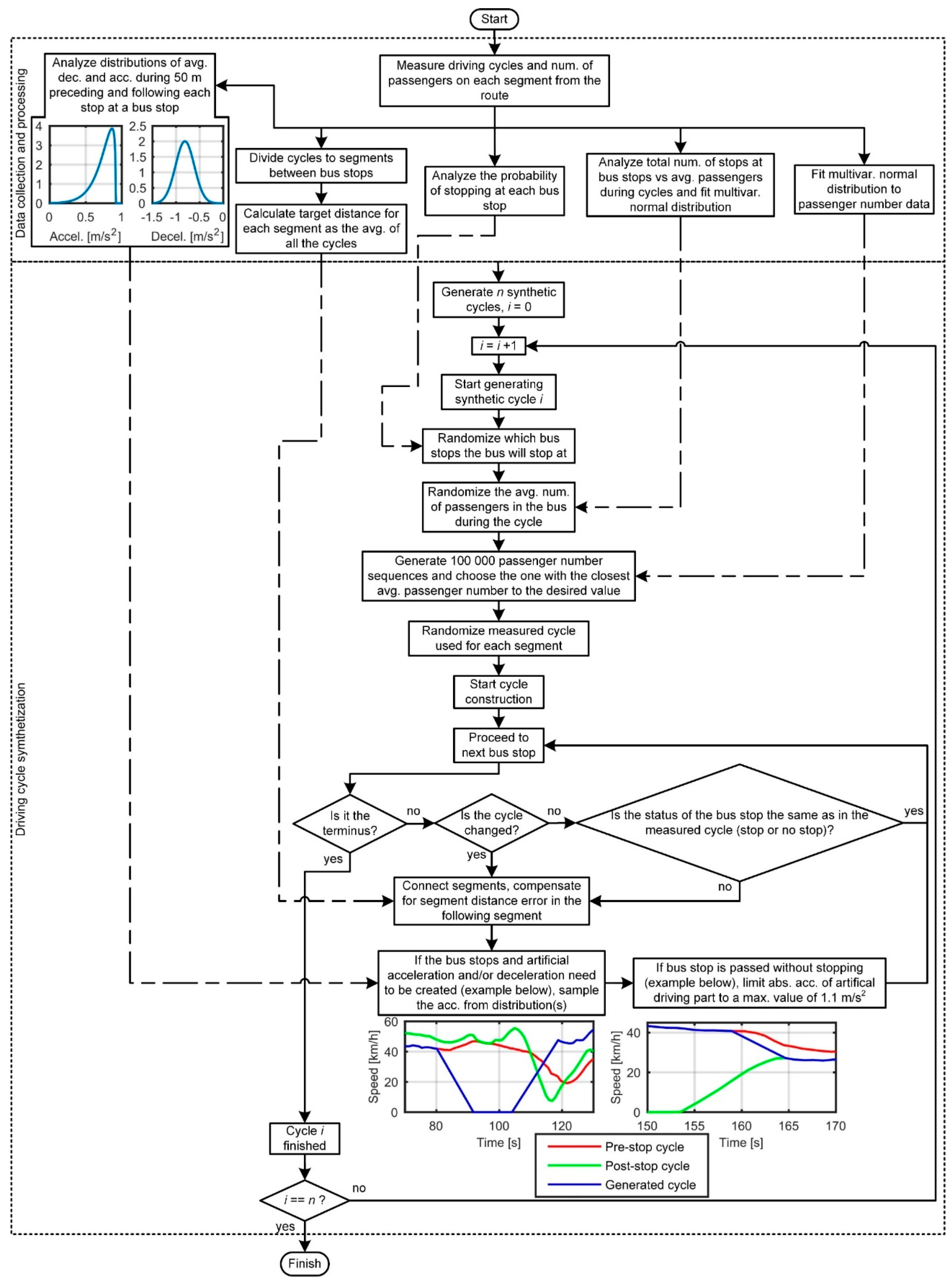
3.1. Driving Cycle Synthesis Using Monte Carlo Method

In order to acquire a large quantity of varying driving cycles for a single bus route, a driving cycle synthetization method was used. In the synthesis process, which is described in the flowchart in Figure 2, new driving cycles are generated for a selected bus route in a segment-based cut-and-paste process that uses actual measured driving cycles from the route as its basis. In this process, a segment is considered to be the driving profile between two consecutive bus stops. In the synthetic cycles, the measured cycle used for each segment is randomized, and only the respective segments can be chosen (e.g., for the third segment in the synthetic cycle, only the third segments in the measured cycles can be chosen). The bus stops at which the vehicle will stop at during the cycle are randomized, as are the passenger numbers, with both being based on the probabilities found in the measured cycles. The mass of a passenger was defined as 68 kg in this study as per Federal Transit Administration (FTA) bus testing regulations [24].
The distance of each synthetic cycle created for the same route is kept the same by compensating for distance variations when connecting the segments. Each segment has a target distance, and the difference between the target and the actual distance is added to the next segment. Thus, the individual segment lengths can vary slightly, but the total distance remains constant. When a bus stop is artificially skipped, the speed peaks preceding and following the bus stop are connected together. The maximum absolute value of the acceleration in such artificial driving portions was set to 1.1 m/s2. This value was chosen based on previous works regarding passenger safety and comfort [25,26]. In the artificial stop maneuvers, and the deceleration and acceleration, which are sampled from distributions based on the measurements, are constant. This was considered to be reasonable, as the highest speed limit on the route is 60 km/h, and thus the acceleration power demand will not become excessive even at the highest speeds.
The bus line examined in this study is line 11 in Espoo, Finland (Figure 3). The line, which includes 25 bus stops, features a typical suburban bus route and had been operated by electric buses. The direction from Friisilä to Tapiola was considered, and 24 driving cycles were acquired between 27 December 2016 and 6 February 2017 from a BEB operating on the route. The bus is of the same model as the BEB that is described in Section 3.3. The measurements were used as the basis of the driving cycle synthetization process. The speed signal from the anti-lock brake system was used with a sampling rate of 1 Hz. In order to determine which bus stops the vehicle stopped at, the Global Positioning System (GPS) coordinates of the bus were logged. Passenger numbers had to be measured separately by logging them manually inside the bus. Passenger numbers were measured on 37 runs of the route between March 2016 and February 2017. The average number of passengers in the bus during a cycle was 6.1. The highest average amount of passengers in the bus on any cycle was 12.1, and the lowest value was 2.3. The peak number of passengers observed was 29.
The characteristic parameters of the Espoo 11 (E11) route are compared with those of the well-known Braunschweig (BR) bus test cycle in Table 2. Although the BR cycle represents urban driving, it was still considered to be a good comparison point because of its relatively similar characteristics and widespread use in literature, such as in the works of [2,14,27,28]. The parameter list was adapted based on previous studies [2,29]. The parameters presented for the E11 route are the averages of the values calculated for each of the measured cycles.
The aggressiveness was calculated as follows [30]:
  A = i = 1 n t i , 1 t i , 2 ( a · v )   d t / s ,
where a is the positive (forward) acceleration and v the speed of the bus, n is the number of positive acceleration periods, t i , 1 and t i , 2 are the start and end of the i -th positive acceleration period, and s is the distance of the entire driving cycle. Creep and cruise were defined as follows:
  • Creep: 0 < v 4   km / h   &   | a | 0.1   m / s 2
  • Cruise: v > 4   km / h   &   | a | 0.1   m / s 2
Figure 4 features an example driving cycle from the E11 route, as well as the BR cycle. The altitude profile of the E11 route is included in the figure. The purple lines in Figure 3 and Figure 4 indicate the areas of the route with high density urban dwellings. These areas tend to feature higher traffic. The altitude of the terminus is 0.5 m lower than that of the starting point. At its highest point, the route is 14.7 m above sea level, and at the lowest point, it is 2.0 m above sea level. The steepest positive road inclination angle (uphill) on the route is approximately 4.0 degrees and the steepest negative angle (downhill) is approximately −3.6 degrees. The average uphill angle is 0.4 degrees and average downhill angle −0.5 degrees.
In order to compare the influence of driving cycle and passenger load variations on different city bus powertrain configurations with simulation studies, 3000 unique synthetic cycles and passenger number sequences were generated. The number of cycles is further discussed at the end of Section 3.3. An example of a synthetic E11 cycle is shown in Figure 5. The statistical distributions of the parameters of the 3000 synthetic cycles are presented in Table 3.
The validity of the cycle synthesis method was confirmed by comparing the speed-acceleration probability distributions (SAPD) of the 24 measured cycles and the 3000 synthetic cycles. Figure 6 shows that there were only minor differences between the SAPDs. Furthermore, the Pearson correlation coefficient between the number of stops and average passenger load during a cycle was 0.605 in the measured cycles, and 0.555 in the synthetic cycles, showing that the synthetic passenger loads correlated with the frequency of stops in a realistic manner.

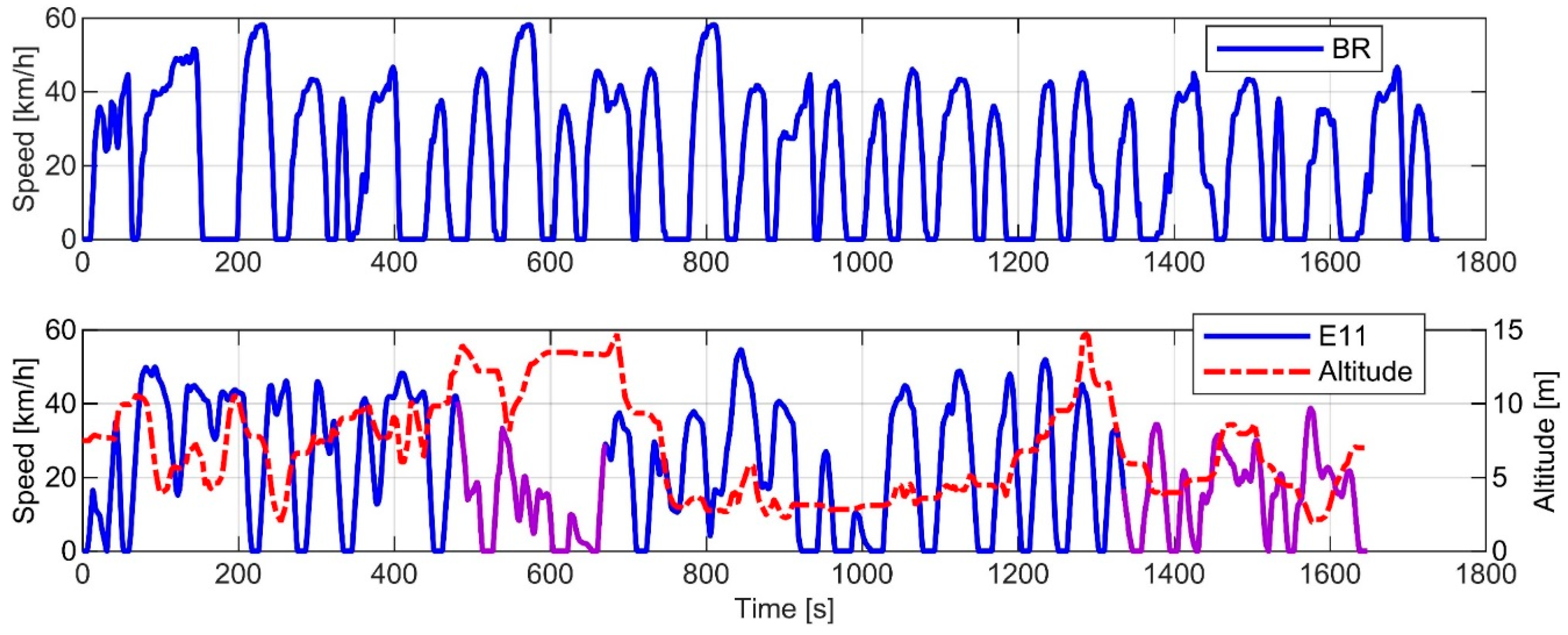
3.2. Reference Driving Cycles

Various bus driving cycles were gathered in order to examine how the results obtained from the single route simulations would relate to results acquired from a more varied set of driving cycles. Their characteristic parameters are presented in Table 4. The total number of different cycles was 20, which also included the BR cycle.
Cycles from lines B18 and B51 in Berkeley, California had been used by Lajunen and Lipman in a previous study [2]. The alternative Espoo 11 cycle (E11B) was used in the same study, as was the Helsinki 550 (H550) cycle. The H550 bus line contains a mix of suburban and urban driving in the Helsinki region.
The Helsinki 1 (H1), Helsinki 2 (H2), and Helsinki 3 (H3) bus test cycles were presented in a heavy-vehicle energy efficiency report by Nylund et al. [31]. The H1 cycle features urban and exit road driving while the H2 cycle only contains urban driving. The H3 cycle contains exit road and ring road driving.
The Helsinki 24 (H24), Turku 03 (TU03), and Tampere 25 (TA25) cycles were measured from the bus lines by Liimatainen et al. [32]. Each of the three lines feature both urban and suburban driving sections. The Helsinki 55 (H55), Helsinki 58 (H58), Lahti 05 (L05), and Lahti 31 (L31) cycles were acquired from buses operating on the lines. H55 and H58 feature both urban and suburban sections, while the Lahti cycles only feature suburban driving.
The Manhattan bus cycle (MAN) and New York bus cycle (NYC) are widely-used test cycles that represent bus driving in downtown Manhattan. The Orange County cycle (OCC) is another commonly used test cycle. It was developed based on driving patterns of urban transit buses in the Los Angeles, California area [33]. The Nuremberg R36 cycle and the RTE cycle feature urban driving. The RTE cycle, which was measured in Denver, CO, USA and is available in Autonomie by default, has the highest number of stops per kilometer of all the cycles. Figures of the cycles can be found in Appendix A. For these simulated cycles, the payload was set to 440 kg, which was the average passenger load in the synthetic cycles.

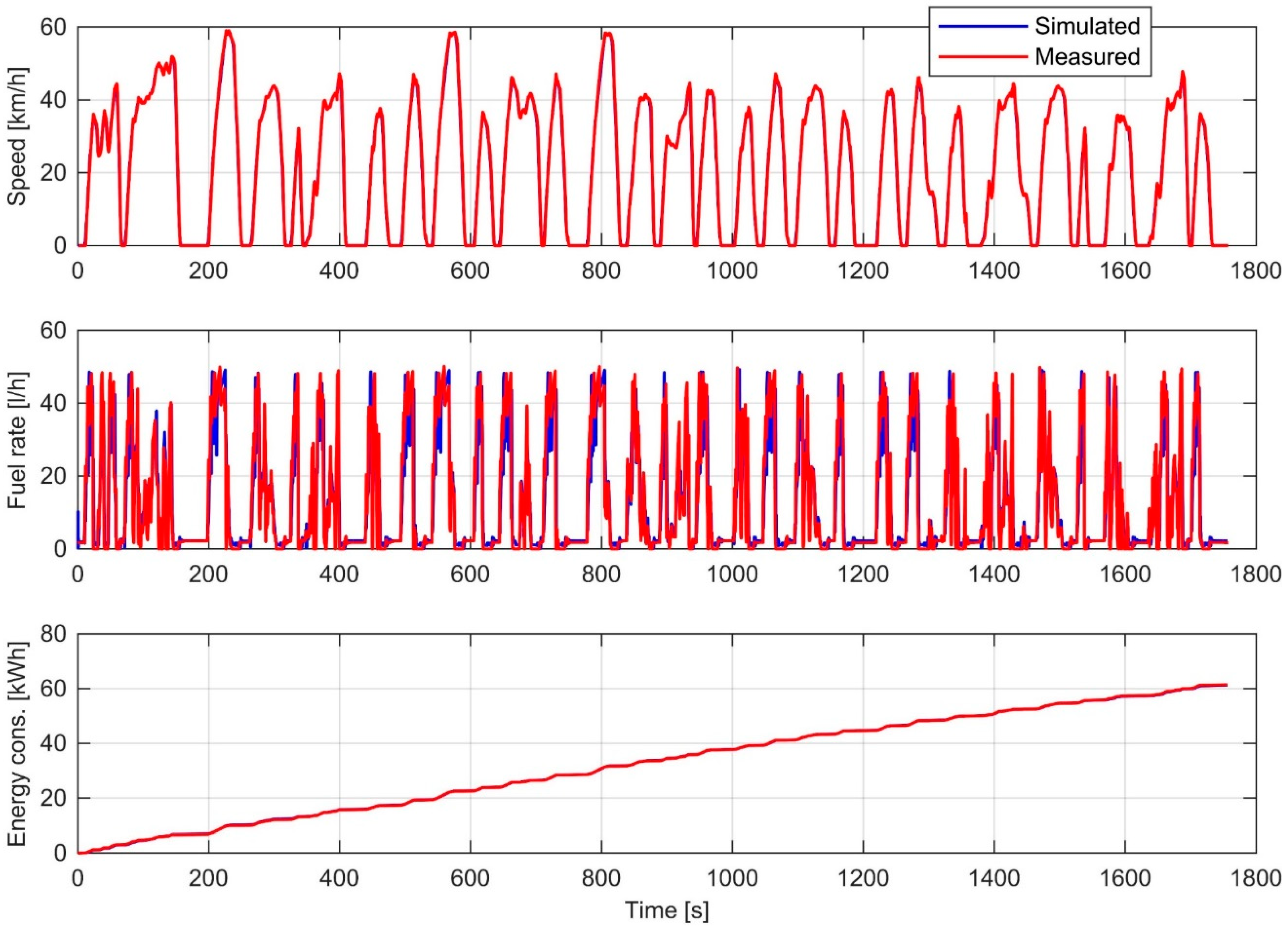
3.3. Simulation Models

Autonomie vehicle simulation software (revision 14), developed by Argonne National Laboratory (Lemont, IL, USA), was used in this study. The software is based on MATLAB (version R2012a), and it provides a framework for automotive control-system design, simulation, and analysis [34]. The software includes predefined powertrain architectures and libraries for powertrain components. Component initialization data is also provided, including those for heavy vehicles [35].
The six different bus models were based upon those used in Lajunen and Lipman [2]. The parallel hybrid model is of the pre-transmission kind, meaning that the electric motor is coupled with the engine at the gearbox input shaft. The hybrid electric, FCH, and battery electric buses all use lithium-ion battery packs. None of the hybrid models feature plug-in charging functionality. Plug-in models would require a separate comprehensive analysis because of their energy consumption being significantly influenced by the battery capacity and control strategy.
As measurement data was available from a battery electric bus and a diesel bus, the respective simulation models were modified to match the buses. The modified models were validated by comparing simulated and measured quantities. Diesel bus dynamometer data was acquired from VTT Technical Research Centre of Finland. The laboratory has up-to-date calibrated chassis dynamometer and measurement procedures. The measurement procedures have been accredited. The dynamometer test simulated the Braunschweig cycle. The sampling rate of the measurements was 10 Hz. In the test, the bus had a payload of 4750 kg. The curb weight of the bus is 14,750 kg. Hence, the total mass was 19,500 kg, and the mass of the simulation model was set to the same value for the validation. The energy consumption was calculated based on fuel flow data with the density of diesel fuel assumed to be 0.835 kg/L and the heating value 42.5 MJ/kg as per the default values provided by Autonomie. A comparison of the fuel rate and of the cumulative energy consumption between the measured cycle and the simulated cycle is presented in Figure 7. The root-mean-square error (RMSE) of the simulated fuel rate was 5.06 L/h. The simulated energy consumption was 61.26 kWh, and the measured consumption was 61.44 kWh, meaning that the error was 0.3%. The average ambient temperature during the measurements was 23.0 °C.
Onboard measurement data was acquired from an electric bus (Figure 8) operating on bus line 55 in Helsinki. The examined driving cycle is the H55 cycle presented in Table 4. The number of passengers during the cycle was acquired from the Helsinki Region Transport (HSL). The average mass of a passenger was again estimated to be 68 kg. The sampling rate of the measurements was 0.2 Hz. The average ambient temperature during the cycle was 22.4 °C.
The powertrain of the battery electric bus simulation model was modified to match the one in the actual bus, and the model was validated. The opportunity-charging type BEB features a lightweight aluminum chassis, and its curb weight is 10,500 kg [36]. Figure 9 shows the state-of-charge (SOC) of the battery pack during the measured and simulated cycle, as well as the speed and altitude. The SOC was estimated using Coulomb counting in both the actual bus and the simulation model. The total SOC change during the measured cycle was 23.04%, and during the simulated cycle, it was 23.02%. The RMSE of the simulated SOC was 0.52%. It can be seen in Figure 9 that the simulated SOC deviates slightly from the measured value during the first half of the cycle up to a maximum difference of 1.20%, and then during the second half, the simulated and measured values converge again. This was presumed to be a result of inaccuracy in the altitude profile, as the cycle featured the full route of the Helsinki 55 bus line.
The validated electric powertrain, excluding the battery pack, was also implemented into the series hybrid and fuel cell hybrid bus simulation models. The powertrain specifications of the simulation models can be found in Table 5. In order to acquire a fair comparison for the six different powertrain configurations, the masses of each of the bus models were reconfigured using the mass of the electric bus as the baseline. The relative differences between the masses of the powertrains were determined based on available bus model specifications. Based on the works of [37,38,39], it was estimated that diesel, parallel hybrid, and battery electric bus powertrains weigh approximately the same amount if the battery electric configuration is of the opportunity-charging type with a relatively light battery pack. Hence, the curb weights of the three models were set equal. The differences between the masses of the series hybrid, CNG, and diesel buses were approximated based on the work of [40]. The FCH powertrain was estimated to weigh 1630 kg more than the diesel powertrain based on bus specifications found in an FCH bus operation report by Eudy and Post [41].
The chassis dimensions, as well as the frontal area, drag coefficient, and rolling resistance coefficients, were all defined as the same for each model (Table 6). The ambient temperature was set to 22.5 °C for the simulations. The speed and deceleration limits for regenerative braking modes for the parallel hybrid, series hybrid, FCH, and battery electric bus models are presented in Table 7. When the conditions for both modes are met, full regeneration mode is preferred.
In order to acquire a reference level for the energy consumption of each of the six different vehicles, the BR cycle was run with the models both with no extra load and with an extra load of 1000 kg. Figure 10 shows the energy consumption variations caused by the load.
On the Braunschweig cycle tests, the CNG bus had on average approximately 15% higher energy consumption than the diesel bus. The series hybrid consumed approximately 2% less energy than the parallel hybrid and 30% less than the diesel bus. The mean consumption of the FCH bus was 25% lower than that of the series hybrid, and the BEB consumed approximately 57% less energy than the FCH. The effect of the 1000 kg of mass was approximately 0.25, 0.24, 0.19, 0.17, 0.13, and 0.05 kWh/km for the CNG, diesel, parallel hybrid, series hybrid, FCH, and BEB, respectively.
As was mentioned in Section 3.1, 3000 synthetic cycles were generated. The average energy consumption of the diesel bus was plotted as a function of the number of simulated cycles in order to examine the sufficiency of the number of synthetic cycles (Figure 11).
As can be seen in Figure 11, there was significant variation in the average consumption during the first 500 cycles. During the final 500 cycles, the value only varied between 3.5920 and 3.5905 kWh/km. Hence, it can be stated that 3000 cycles produce statistically reliable results.

4. Results and Discussion

4.1. Synthetic Suburban Cycle Simulations

The energy consumption histograms of the 3000 synthetic E11 cycles are presented in Figure 12 and the distribution statistics in Table 8. The coefficient of variation (CV), which describes the statistical dispersion of the data, is calculated by dividing the standard deviation with the mean.
The results show that the CNG bus consumed on average 14.2% more energy than the diesel bus. This is consistent with previous studies, which have shown that CNG buses are more energy-consuming than diesel buses because of lower engine efficiency [2,20]. CNG engines could potentially be closer to diesel engines in terms of energy consumption in series hybrid configurations. This is because CNG engines would benefit more from being operated only at their most efficient operating point because of higher variation in the efficiency map.
The results demonstrate the significant energy consumption reductions that hybrid powertrains can yield compared with conventional powertrains. Even the hybrid bus that had the highest consumption, the parallel hybrid, consumed 30% less energy on average than the diesel bus. The series hybrid consumed approximately 5% less energy on average than the parallel hybrid. However, the CV of the consumption was slightly lower with the parallel hybrid than with the series hybrid. The BEB had the lowest energy consumption by a large margin; even the FCH consumed 130% more energy on average. Furthermore, the BEB had the lowest statistical dispersion of the consumption, which demonstrates that the battery electric powertrain is the most resistant of the six compared powertrains to variations in the driving cycle on a typical suburban driving route. The lower variation compared with the hybrid powertrains is mostly due to the battery electric powertrain lacking the kind of relatively inefficient component (i.e., ICE, engine-generator, or fuel cell) that the hybrid powertrains need to deploy to a varying extent depending on the driving cycle.
The regenerative braking efficiency was calculated as the ratio of energy stored into the battery and the energy wasted as heat with the brakes during periods when negative power was provided to the driven wheels. The parallel hybrid powertrain was left out of this comparison because of the fact that the ICE would occasionally provide positive torque during light braking maneuvers depending on the SOC of the battery, which would skew the calculated efficiency. The efficiency histograms are presented in Figure 13 and the statistics in Table 9.
The regenerative braking efficiency results show that the BEB was slightly more efficient at regenerating the energy than the series or FCH buses. This is because of the lower mass of the battery electric powertrain, as the regeneration power demand would exceed the limits of the motor less frequently. Additionally, the mass generally influences the operation point during the regeneration. The FCH bus had the lowest efficiency, as it is the heaviest of the three because of the hydrogen tank.
In order to assess the effect that the various cycle parameters had on the energy consumption of each powertrain, the Pearson correlation coefficients were calculated for the parameters and the consumption. The coefficients are presented in Table 10. In the table, the coefficients have been ordered from highest to lowest based on the average absolute values of the coefficients.
The results demonstrate that aggressiveness, as defined in Equation (1), is a robust way of describing the energy demand of a driving cycle, as it had the highest correlation with the consumption on average. Comparing the conventional powertrains, the diesel bus appears to have been slightly more sensitive to aggressiveness than the CNG bus, which is an interesting result, especially considering the higher mass of the CNG powertrain. The result can be explained by the differences in the efficiency maps, as the diesel engine model has a more consistent efficiency in the usual operating region, meaning that more aggressive driving maneuvers could result in a comparatively higher efficiency increase with the CNG engine. On the other hand, the consumption of the CNG bus correlated stronger with the frequency of stops. This phenomenon is at least in part explained by the CNG bus consuming more energy during idling because of a lower efficiency at that operating point. This can also be seen in the correlation between the average stop duration and the consumption. The efficiency during idling was approximately 25% with the diesel engine and approximately 15% with the CNG engine. Such a large difference is not necessarily universally true for all CNG and diesel bus engines, but instead is specific to the engine models used in this study.
The differences between the three hybrid buses were mostly small. The parallel hybrid was slightly less sensitive to the aggressiveness of the cycle than the series hybrid and FCH buses, but it was more sensitive to the stop frequency and especially to the average speed and driving speed. The slightly lower sensitivity to aggressiveness and average acceleration of the parallel hybrid may have been due to the ICE being directly connected to the wheels, and hence more aggressive maneuvers could increase the efficiency of the ICE. With electric motors, the efficiency is more constant. The electric motor in the parallel hybrid is also less powerful than those of the other hybrids and the BEB. This means that the regeneration will be more often limited by the maximum power of the motor, thus making the parallel hybrid waste more energy as heat in braking maneuvers.
Table 10 clearly shows that the passenger load was less significant to the consumption than the driving cycle. Part of the reason for this is that the examined bus line is not particularly busy. The correlation between the average passenger load and the consumption was similar with each model. The correlation was slightly higher with the diesel bus than with the CNG bus, which was likely due to the CNG bus being heavier and thus the passenger load being proportionally a smaller increase in the total mass. For the same reason, the correlation was higher with the BEB than with the FCH bus, and with the FCH bus, it was higher compared with the series hybrid bus, all three of which share the same electric powertrain, except for the battery pack.
The cycle parameters are inherently connected to one another and thus correlate with each other. In order to try to evaluate the uncorrelated effect of the cycle parameters on the consumption, the multiple linear regression analysis method presented by Xu and Gertner [42] was used. The method is based on using variance decomposition to separate the correlated and uncorrelated portion of the effect. The correlation in this context means the correlation between the different examined factors. The five most influential parameters as per Table 10 plus the average passenger load were examined in the analysis. The analysis is presented in Figure 14. A limited parameter selection was used, as examining all the parameters at once would cause the calculated uncorrelated influence of the parameters to be negligible. This is because of how strongly all of the different cycle properties correlate with each other.
It can be seen in Figure 14 that aggressiveness had the highest amount of uncorrelated influence on consumption. Aggressiveness had the highest amount of uncorrelated influence on consumption of the diesel bus (15.88%) and the lowest amount on consumption of the parallel hybrid (9.28%). The results indicate that, between the conventional bus types, the diesel bus is more sensitive to aggressiveness of the driving maneuvers. Among the hybrids, the parallel hybrid appears the least influenced by aggressiveness based on these results. The average passenger load had the highest amount of uncorrelated influence on the consumption of the BEB (6.64%) and the lowest on the consumption of the CNG bus (2.54%). The results are indicative of the fact that the passenger load is proportionally less significant with the conventional bus powertrains than with the hybrid and battery electric powertrains. This is because the driving cycle properties are comparatively more influential with the conventional models because of the lower and more varying tank-to-wheels efficiency and the lack of regenerative braking.

4.2. Reference Cycle Simulations

The energy consumption statistics of the six bus models on the driving cycles presented in Section 3.2 are shown in Table 11. It should be noted that the analysis only included 19 cycles instead of 20, as the NYC cycle had to be rejected because of the parallel hybrid bus being unable to complete it without a significant decrease in the SOC level. Additionally, the B18 cycle had to be completed in two parts with the BEB, as the battery pack did not have a high enough capacity to complete such a long route on a single charge.
The results are mostly consistent with those acquired with the synthetic E11 cycles. However, it can be seen that this time, the parallel hybrid bus had a significantly higher statistical dispersion of the consumption compared with the other hybrids. The maximum consumption, which occurred on the RTE cycle, was also substantially higher compared with the other hybrid buses. On city center type cycles, with high aggressiveness and frequent stops, the parallel hybrid started to struggle to maintain the SOC of the battery pack at a constant level. The issue was that the amount of energy that could be regenerated during braking was more limited because of the lower speeds. Furthermore, there were limited opportunities to charge the battery during acceleration because of the ICE already delivering close to maximum power for propulsion. Hence, the electrical auxiliary device power demand was nearly as high as the average regeneration power. Thus, the electric motor was barely used for propulsion at all. As mentioned earlier, on the NYC cycle, the regeneration opportunities were so limited that the SOC could not be maintained at a constant level. Further examination of the results indicated that the consumption of the parallel hybrid started to increase more compared with the series hybrid on cycles with above 2.5 stops per km and 0.23 m/s2 aggressiveness. These results demonstrate that parallel hybrid buses are not well-suited for low-speed city center stop-and-go type driving.
Mild hybrid powertrains were not considered in this study because of a lack of availability of up-to-date models and validation data. Mild hybrids use the parallel hybrid powertrain configuration and do not feature an exclusive electric-only mode of propulsion. The electrical energy storage capacity in mild hybrids is significantly lower than in parallel (full) hybrids, and the electric motor is less powerful [43]. It is assumed that, depending on the degree of hybridization, they would fall somewhere between the diesel and parallel hybrid models, both in terms of mean energy consumption and the dispersion of the consumption. In Lajunen [14], a mild hybrid bus featuring ultracapacitors and a 75 kW electric motor was shown to consume more energy than a parallel hybrid bus, but still substantially less than a conventional diesel bus when compared on a few different driving cycles. On the lowest-consuming cycle, the consumption of the mild hybrid was almost on par with that of the parallel hybrid, but on the highest-consuming cycle, it was about halfway between the parallel hybrid and diesel buses.
The correlation coefficients between the cycle parameters and the consumption on the 19 cycles are shown in Table 12.
As can be seen in the table, the stop frequency on these cycles had the highest correlation with the consumption. Average deceleration also had a slightly higher correlation with the consumption compared with the E11 cycles. Additionally, the maximum speed of the cycle correlated more with the consumption, as with a broader variety of cycles, the maximum speed is correlated more with the general nature of the cycle, whereas on a single route, it does not have much significance. One notable result is that the correlation between the consumption and the aggressiveness was slightly lower with the parallel hybrid than the series hybrid, which could seem to contradict the earlier explanation about the consumption of the parallel hybrid on aggressive cycles. However, this may simply be because the correlation between aggressiveness and the energy consumption of the parallel hybrid was somewhat exponential with high aggressiveness values, while the Pearson coefficient is a measure of linear correlation. The assumption of linearity is one of the weaknesses of this type of analysis. Additionally, the sample size of 19 cycles is relatively low, and that affects the reliability of the results. A variance decomposition analysis was conducted for these results as well (Figure 15). The top five parameters in Table 12 were examined.
Compared with the E11 route results, the variance decomposition shows that the aggressiveness had less uncorrelated influence on the consumption. This is partially because average deceleration is now included in the five parameters, which had high correlation with aggressiveness (−0.90). However, even when swapping the average deceleration to average speed, the uncorrelated influence of the aggressiveness only varied between 2.64% and 4.95%. This is because there was more significant variation in the other aspects of the cycles compared with the Espoo suburban single-route driving cycles. Hence, aggressiveness also correlated more with the other properties. Nonetheless, similar trends to the Espoo 11 synthetic cycle results can be seen. Aggressiveness had a lower uncorrelated influence again to the energy consumption of the CNG bus than to that of the diesel bus. It also again had lower uncorrelated influence to the consumption of the BEB than the FCH bus.
Based on the results of this comprehensive energy consumption study, a brief summary of the consumption-related advantages and disadvantages of each of the six city bus powertrains is presented in Table 13.

5. Conclusions

In this paper, the sensitivity of the energy consumption of the most common city bus powertrain topologies to driving cycle and passenger load variations was analyzed. Three-thousand varying synthetic cycles and passenger number sequences were generated for a typical suburban bus route based on cycles and passenger numbers measured from a route in Espoo, Finland. Additionally, twenty reference driving cycles featuring various types of driving were simulated. The cycles were simulated with six different bus models, including diesel, CNG, parallel hybrid, series hybrid, FCH, and battery electric buses. The electric powertrain used in the hybrids and the BEB was validated based on measurement data, as was the diesel powertrain. The masses of the models were configured such that the chassis was assumed to be the same with each model. The correlations between the various cycle parameters and the energy consumption were analyzed. Further examination was conducted using variance decomposition analysis to investigate the uncorrelated effects of the parameters. Novel comparative data about the influence of cycle characteristics on the energy consumption of city buses was acquired.
Firstly, the results demonstrated that the aggressiveness parameter, which has thus far been seldom used in publications, is an effective way to characterize the energy demand of a driving cycle, as it had the highest correlation with consumption in the synthetic cycles and the second highest behind stop frequency in the measured cycles. The way aggressiveness is formulated in Equation (1) puts particular emphasis on high-speed acceleration maneuvers. Hence, one implication of the results is that particular attention should be paid to limiting high-speed accelerations of buses in order to minimize energy consumption. The passenger load variations were found to be substantially less influential to the consumption than the variations in the driving cycle. Heavier powertrains were proportionally less affected by the passenger load as a result of the load being comparatively a smaller increase in the total mass of the bus. Thus, it can be stated that the more crowded the bus line is, the more competitive the heavier powertrain options are in terms of energy consumption.
The results showed that the CNG bus had a higher energy consumption, as well as higher consumption dispersion, compared with the diesel bus. The results also indicated that diesel buses are the most sensitive to the aggressiveness of the driving. Therefore, it is particularly important to provide coaching or assistance systems for drivers of diesel buses in order minimize the aggressiveness of their driving styles, thus minimizing energy use and pollution. An examination of the hybrid bus consumptions showed that the parallel hybrid had a lower statistical dispersion of the consumption, but a higher mean consumption than the series hybrid on the Espoo suburban cycles. On the other hand, on the collection of more varied types of cycles, the parallel hybrid had a significantly higher dispersion and maximum consumption. This was because the parallel hybrid could not make full use of the versatility of its powertrain when the aggressiveness and stop frequency of the cycle increased beyond a certain point. Based on this result, it is strongly recommended for transit agencies to pay close attention to which kinds of routes parallel hybrid buses are deployed on. On suitable routes, they may offer a more consistent energy consumption than series hybrid buses, but on too aggressive cycles, they will be highly inefficient and, at worst, may even be unusable, as was seen with the NYC driving cycle in this study. The severity of this issue could potentially be reduced by designing parallel hybrid buses in a way that would allow taking a larger portion of the auxiliary device power from the engine in cases where regeneration opportunities are severely limited.
The BEB had the lowest consumption and consumption dispersion in the simulations, which demonstrates that this topology is the most resistant one against driving cycle variations. Additionally, the analysis showed that the energy consumption of the battery electric powertrain was less sensitive to the aggressiveness of the driving compared with the series and fuel cell hybrid powertrains.
Future research is needed to better understand how the specifications and component choices of the different topologies might alter the results. Additional parameters should also be examined, especially the energy consumption influence of ambient temperature and weather conditions and their interactions with the driving cycle.

Author Contributions

K.K. acquired the validation data, performed the model validations and simulations, analyzed the results, and wrote the paper. A.L. and K.K. built the simulation models. J.V. proposed the use of variance decomposition analysis and implemented it in MATLAB. K.T. supervised the project and helped with funding acquisition. A.L., J.V., and K.T. provided feedback on the original draft of the paper.

Funding

Funding for this study was provided by the Finnish Funding Agency for Technology and Innovation, Tekes, through the Batteries for Business project. Furthermore, Yrjö and Senja Koivunen and Henry Ford foundations provided a grant for this research.

Acknowledgments

The authors would like to thank Linkker Ltd. and Sami Ruotsalainen for providing support and data for the study. We also wish to express our gratitude to VTT Technical Research Centre of Finland Ltd. and HSL for providing dynamometer and traffic data.

Conflicts of Interest

The authors declare no conflict of interest.

Appendix A. Driving Cycles

In this appendix, the bus driving cycles used in the simulations that were not shown in Section 3 are presented. The cycles have been grouped together into four figures based on their durations.
Figure A1. City bus driving cycles with a maximum duration of 1300 s.
Energies 11 01755 g0a1
Figure A2. City bus driving cycles with a maximum duration of 2200 s.
Energies 11 01755 g0a2
Figure A3. City bus driving cycles with a maximum duration of 4500 s.
Energies 11 01755 g0a3
Figure A4. Berkeley bus line 18 driving cycle.
Energies 11 01755 g0a4

References

  1. Nylund, N.-O.; Koponen, P. Fuel and Technology Alternatives for Buses: Overall Energy Efficiency and Energy Performance; VTT: Espoo, Finland, 2012. [Google Scholar]
  2. Lajunen, A.; Lipman, T. Lifecycle cost assessment and carbon dioxide emissions of diesel, natural gas, hybrid electric, fuel cell hybrid and electric transit buses. Energy 2016, 106, 329–342. [Google Scholar] [CrossRef]
  3. Zhu, T.; Min, H.; Yu, Y.; Zhao, Z.; Xu, T.; Chen, Y.; Li, X.; Zhang, C. An Optimized Energy Management Strategy for Preheating Vehicle-Mounted Li-ion Batteries at Subzero Temperatures. Energies 2017, 10, 1–23. [Google Scholar] [CrossRef]
  4. Leou, R.C.; Hung, J.J. Optimal Charging Schedule Planning and Economic Analysis for Electric Bus Charging Stations. Energies 2017, 10. [Google Scholar] [CrossRef]
  5. Kim, J.; Song, I.; Choi, W. An Electric Bus with a Battery Exchange System. Energies 2015, 8, 6806–6819. [Google Scholar] [CrossRef] [Green Version]
  6. Cheng, S.; Xu, L.; Li, J.; Fang, C.; Hu, J.; Ouyang, M. Development of a PEM Fuel Cell City Bus with a Hierarchical Control System. Energies 2016, 9. [Google Scholar] [CrossRef]
  7. Eudy, L.; Post, M. Fuel Cell Buses in U.S. Transit Fleets: Current Status 2017; National Renewable Energy Laboratory: Golden, CO, USA, 2017.
  8. Wang, J. Barriers of scaling-up fuel cells: Cost, durability and reliability. Energy 2015, 80, 509–521. [Google Scholar] [CrossRef]
  9. Carignano, M.; Adorno, R.; van Dijk, N.; Nieberding, N.; Nigro, N.; Orbaiz, P. Assessment of Energy Management Strategies for a Hybrid Electric Bus. In Proceedings of the 5th International Conference on Engineering Optimization, Iguassu Falls, Brazil, 19–23 June 2016; pp. 19–23. [Google Scholar]
  10. Ehsani, M.; Yimin, G.; Miller, J.M. Hybrid Electric Vehicles: Architecture and Motor Drives. Proc. IEEE 2007, 95, 719–728. [Google Scholar] [CrossRef]
  11. García Sánchez, J.A.; López Martínez, J.M.; Lumbreras Martín, J.; Flores Holgado, M.N.; Aguilar Morales, H. Impact of Spanish electricity mix, over the period 2008–2030, on the Life Cycle energy consumption and GHG emissions of Electric, Hybrid Diesel-Electric, Fuel Cell Hybrid and Diesel Bus of the Madrid Transportation System. Energy Convers. Manag. 2013, 74, 332–343. [Google Scholar] [CrossRef]
  12. Ercan, T.; Zhao, Y.; Tatari, O.; Pazour, J.A. Optimization of transit bus fleet’s life cycle assessment impacts with alternative fuel options. Energy 2015, 93, 323–334. [Google Scholar] [CrossRef]
  13. Bottiglione, F.; Contursi, T.; Gentile, A.; Mantriota, G. The Fuel Economy of Hybrid Buses: The Role of Ancillaries in Real Urban Driving. Energies 2014, 7, 4202–4220. [Google Scholar] [CrossRef] [Green Version]
  14. Lajunen, A. Energy consumption and cost-benefit analysis of hybrid and electric city buses. Transp. Res. Part C Emerg. Technol. 2014, 38, 1–15. [Google Scholar] [CrossRef]
  15. Nesamani, K.S.; Subramanian, K.P. Development of a driving cycle for intra-city buses in Chennai, India. Atmos. Environ. 2011, 45, 5469–5476. [Google Scholar] [CrossRef]
  16. Lai, J.; Yu, L.; Song, G.; Guo, P.; Chen, X. Development of City-Specific Driving Cycles for Transit Buses Based on VSP Distributions: Case of Beijing. J. Transp. Eng. 2013, 139, 749–757. [Google Scholar] [CrossRef]
  17. Zhang, B.; Gao, X.; Xiong, X.; Wang, X.; Yang, H. Development of the driving cycle for Dalian city. In Proceedings of the 8th International Conference on Future Generation Communication and Networking, Haikou, China, 20–23 December 2014; pp. 60–63. [Google Scholar]
  18. Peng, M.; Liu, X.; Lin, Q. Construction of Engine Emission Test Driving Cycle of City Transit Buses. In SAE 2015 Commercial Vehicle Engineering Congress; SAE International: Rosemont, IL, USA, 2015. [Google Scholar]
  19. Ally, J.; Pryor, T. Life cycle costing of diesel, natural gas, hybrid and hydrogen fuel cell bus systems: An Australian case study. Energy Policy 2016, 94, 285–294. [Google Scholar] [CrossRef] [Green Version]
  20. Wang, R.; Wu, Y.; Ke, W.; Zhang, S.; Zhou, B.; Hao, J. Can propulsion and fuel diversity for the bus fleet achieve the win-win strategy of energy conservation and environmental protection? Appl. Energy 2015, 147, 92–103. [Google Scholar] [CrossRef]
  21. Xu, Y.; Gbologah, F.E.; Lee, D.Y.; Liu, H.; Rodgers, M.O.; Guensler, R.L. Assessment of alternative fuel and powertrain transit bus options using real-world operations data: Life-cycle fuel and emissions modeling. Appl. Energy 2015, 154, 143–159. [Google Scholar] [CrossRef]
  22. Correa, G.; Muñoz, P.; Falaguerra, T.; Rodriguez, C.R. Performance comparison of conventional, hybrid, hydrogen and electric urban buses using well to wheel analysis. Energy 2017, 141, 537–549. [Google Scholar] [CrossRef]
  23. Zhou, B.; Wu, Y.; Zhou, B.; Wang, R.; Ke, W.; Zhang, S.; Hao, J. Real-world performance of battery electric buses and their life-cycle benefits with respect to energy consumption and carbon dioxide emissions. Energy 2016, 96, 603–613. [Google Scholar] [CrossRef]
  24. Federal Transit Administration Bus Testing: Calculation of Average Passenger Weight and Test Vehicle Weight. Available online: https://www.federalregister.gov/documents/2012/12/14/2012-30184/bus-testing-calculation-of-average-passenger-weight-and-test-vehicle-weight (accessed on 14 February 2018).
  25. Hoberock, L.L. A survey of longitudinal acceleration comfort studies in ground transportation vehicles. J. Dyn. Syst. 1977, 99, 76–84. [Google Scholar] [CrossRef]
  26. Karekla, X.; Tyler, N. Reducing non-collision injuries aboard buses: Passenger balance whilst walking on the lower deck. Saf. Sci. 2018, 105, 128–133. [Google Scholar] [CrossRef]
  27. Halmeaho, T.; Rahkola, P.; Tammi, K.; Pippuri, J.; Pellikka, A.-P.; Manninen, A.; Ruotsalainen, S. Experimental validation of electric bus powertrain model under city driving cycles. IET Electr. Syst. Transp. 2016, 7, 74–83. [Google Scholar] [CrossRef]
  28. Kim, M.; Jung, D.; Min, K. Optimal torque distribution strategy for dual traction motors in a series hybrid electric intra-city bus. Int. J. Heavy Veh. Syst. 2017, 24, 18–44. [Google Scholar] [CrossRef]
  29. Amirjamshidi, G.; Roorda, M.J. Development of simulated driving cycles for light, medium, and heavy duty trucks: Case of the Toronto Waterfront Area. Transp. Res. Part D Transp. Environ. 2015, 34, 255–266. [Google Scholar] [CrossRef]
  30. Lajunen, A.; Kalttonen, A. Investigation of Thermal Energy Losses in the Powertrain of an Electric City Bus. In Proceedings of the 2015 IEEE Transportation Electrification Conference and Expo (ITEC), Dearborn, MI, USA, 14–17 June 2015. [Google Scholar]
  31. Nylund, N.-O.; Erkkilä, K.; Westerholm, M. Raskaan Ajoneuvokaluston Energiankäytön Tehostaminen—Raportti 2004; VTT: Espoo, Finland, 2005. [Google Scholar]
  32. Liimatainen, H.; Metsäpuro, P.; Ikonen, M.; Wahlsten, R.; Lajunen, A. Hybridibussit—Kokemuksia Käyttöönotosta, Liikennöinnistä ja Energiankulutuksesta; Tampereen teknillinen yliopisto Liikenteen tutkimuskeskus Verne: Tampere, Finland, 2014. [Google Scholar]
  33. DieselNet Orange County Bus (OC BUS) Cycle. Available online: https://www.dieselnet.com/standards/cycles/ocbus.php (accessed on 8 May 2018).
  34. Argonne National Laboratory Autonomie. Available online: https://www.autonomie.net/expertise/Autonomie.html (accessed on 13 February 2018).
  35. Vijayagopal, R.; Rousseau, A. System Analysis Using Multiple Expert Tools. In SAE World Congress; SAE International: Detroit, MI, USA, 2011. [Google Scholar]
  36. Linkker Technology. Available online: http://www.linkkerbus.com/technology/ (accessed on 14 February 2018).
  37. Volvo Bus Corporation. Volvo 7900 Hybrid Specifikationer. Available online: http://www.volvobuses.se/sv-se/our-offering/buses/volvo-7900-hybrid/specifications.html (accessed on 8 May 2018).
  38. Volvo Bus Corporation. Volvo 7900 Electric Specifikationer. Available online: http://www.volvobuses.se/sv-se/our-offering/buses/volvo-7900-electric/specifications.html (accessed on 8 May 2018).
  39. Volvo Bus Corporation. Volvo 7900 Range—The Volvo 7900 Takes You Further. Available online: https://zahidtractor.com/sites/default/files/7900_range_brochure.pdf (accessed on 8 May 2018).
  40. New Flyer Industries. Xcelsior Specs Sheet. Available online: https://www.newflyer.com/site-content/uploads/2017/09/729-NFL-Xcelsior-Final.pdf (accessed on 8 May 2018).
  41. Eudy, L.; Post, M. Zero Emission Bay Area (ZEBA) Fuel Cell Bus Demonstration Results: Fourth Report Zero Emission Bay Area (ZEBA) Fuel Cell Bus Demonstration Results: Fourth Report; National Renewable Energy Laboratory: Denver, CO, USA, 2015.
  42. Xu, C.; Gertner, G.Z. Uncertainty and sensitivity analysis for models with correlated parameters. Reliab. Eng. Syst. Saf. 2008, 93, 1563–1573. [Google Scholar] [CrossRef]
  43. Daimler Mercedes-Benz Citaro G Hybrid: First Citaro Hybrid Buses Leave the Factory. Available online: http://media.daimler.com/marsMediaSite/en/instance/ko/Mercedes-Benz-Citaro-G-hybrid-First-Citaro-hybrid-buses-leave-the-factory.xhtml?oid=32414377 (accessed on 1 June 2018).
Figure 1. Simplified layouts of different city bus powertrain configurations (AUX = auxiliary devices, BAT = battery, FC = fuel cell, FD = final drive, GB = gearbox, GC = generator and controller, MC = motor and controller, TC = torque coupler).
Energies 11 01755 g001
Figure 2. Driving cycle synthetization flowchart.
Energies 11 01755 g002
Figure 3. Espoo bus line 11, purple sections indicate areas with high density urban dwellings. (Map data ©2018 Google).
Energies 11 01755 g003
Figure 4. Comparison between Braunschweig (BR) and Espoo 11 (E11), purple sections in the E11 cycle indicate areas with high density urban dwellings.
Energies 11 01755 g004
Figure 5. Example of a synthetic Espoo 11 driving cycle and number of passengers.
Energies 11 01755 g005
Figure 6. Speed-acceleration distributions of the measured and 3000 synthetic cycles.
Energies 11 01755 g006
Figure 7. Speed, fuel rate, and cumulative energy consumption during the simulated and actual validation cycle.
Energies 11 01755 g007
Figure 8. Linkker battery electric bus operating in Finland.
Energies 11 01755 g008
Figure 9. Electric bus simulation model validation graphs.
Energies 11 01755 g009
Figure 10. Energy consumption on the BR cycle without load and with a 1000 kg load.
Energies 11 01755 g010
Figure 11. Overall average energy consumption of the diesel bus model versus number of simulated synthetic cycles.
Energies 11 01755 g011
Figure 12. Energy consumption histograms of the simulated synthetic E11 driving cycles.
Energies 11 01755 g012
Figure 13. Regenerative braking efficiency histograms.
Energies 11 01755 g013
Figure 14. Variance decomposition analysis for the six buses on the synthetic E11 cycles.
Energies 11 01755 g014
Figure 15. Variance decomposition analysis for the six buses on the 19 reference cycles.
Energies 11 01755 g015
Table 1. Summary of literature review.
CategoryRef.Authors and YearGeographic ContextMajor Results
Lifecycle cost comparison[2]Lajunen and Lipman, 2016Generic, multiple driving cyclesDiesel hybrid buses are currently the most feasible alternative for conventional buses [2,19].
TCO of FCH buses is more than twice as high as that of diesel buses [2,19].
[19]Ally and Pryor, 2016Perth, Australia
Emissions and optimal fleet composition[11]García Sánchez et al., 2013SpainElectricity production methods and local energy availability strongly influence optimal composition [11,20,21,22].
Viability of BEBs correlates with the amount of congestion in the region [12].
Heterogeneous compositions are better in regions with less energy-demanding driving [12].
Hybrid buses are a robust option for any environment [11,12,20,21,22].
[12]Ercan et al., 2015United States
[20]Wang et al., 2015China
[21]Xu et al., 2015United States
[22]Correa et al., 2017Argentina
Energy consumption and emissions analysis[13]Bottiglione et al., 2014Taranto, ItalyConsumption of hybrids and BEBs is less dependent on the driving cycle compared to diesel and CNG buses [13,14].
Plug-in hybrid buses and BEBs have the highest potential to reduce energy use and emissions [14].
Energy consumption of BEBs and hybrids is more sensitive to auxiliary device power demand [13,23].
[14]Lajunen, 2014Generic, multiple driving cycles
[23]Zhou et al., 2016Macao, China
Table 2. Braunschweig (BR) and Espoo 11 (E11) characteristic parameter comparison.
ParameterBRE11
Max. speed (km/h)58.254.8
Average speed (km/h)22.521.8
Average driving speed (km/h)29.526.2
Distance (km)10.99.74
Stops per km2.62.1
Duration (s)17401637
Total stop time (s)412283
Avg. stop duration (s)14.212.9
Creep percentage1.7%1.8%
Cruise percentage12.8%15.2%
Idle percentage23.7%16.8%
Max. acceleration (m/s2)2.411.44
Max. deceleration (m/s2)3.581.81
Avg. acceleration (m/s2)0.540.46
Avg. deceleration (m/s2)0.720.43
Aggressiveness (m/s2)0.220.19
Table 3. Parameter distribution statistics of the synthetic driving cycles.
ParameterMeanStandard DeviationMaximumMinimum
Max. speed (km/h)56.23.865.447.45
Avg. speed (km/h)21.31.327.016.9
Avg. drv. speed (km/h)25.71.130.721.6
Stops per km2.120.343.390.82
Avg. passengers6.422.3814.570.29
Cycle duration (s)165610220751300
Total stop time (s)29060541115
Avg. stop duration (s)13.42.123.08.3
Creep percentage1.3%0.6%4.3%0.3%
Cruise percentage14.3%2.1%22.8%8.1%
Idle percentage17.4%2.8%28.3%8.8%
Max. acceleration (m/s2)1.480.111.751.11
Max. deceleration (m/s2)1.910.252.761.37
Avg. acceleration (m/s2)0.460.030.570.35
Avg. deceleration (m/s2)0.410.030.510.30
Aggressiveness (m/s2)0.190.010.230.15
Table 4. Bus driving cycle characteristic parameters.
ParameterB18B51E11BH1H2H3H24H55H550H58L05L31MANNYCOCCR36RTETA25TU03
Max. spd (km/h)54.259.058.471.752.571.750.249.474.986.955.459.840.549.365.453.432.556.346.0
Avg. spd (km/h)16.613.623.825.419.641.217.318.230.525.418.822.310.95.919.814.37.220.418.2
Avg. drv. spd (km/h)22.419.727.533.226.547.920.422.935.532.625.227.116.415.924.420.013.624.222.2
Distance (km)42.416.110.27.58.210.37.316.728.730.711.312.43.30.9810.54.32.69.48.9
Stops per km3.34.21.72.03.10.83.42.01.32.61.91.95.710.22.95.410.53.03.8
Duration (s)91774283154810661501902152933053384435421651997108960019091084128916671756
Total stop time (s)23541336412249394125234668472961549355363377355309606262315
Avg. stop dura. (s)16.819.411.415.615.213.99.019.612.412.023.914.218.234.311.512.921.69.09
Creep %4.23.40.10.70.80.30.11.70.10.12.53.51.80.02.90.20.00.20.3
Cruise %11.66.522.210.57.319.09.316.816.87.816.112.08.84.714.47.14.38.910.6
Idle %26.632.413.324.226.813.915.920.414.122.426.118.634.365.319.628.556.916.318.5
Max. acc. (m/s2)1.871.931.601.501.501.422.830.992.031.931.521.812.02.761.811.871.692.844.10
Max. dec. (m/s2)2.211.981.902.332.331.943.821.532.863.141.702.142.492.042.292.102.264.443.95
Avg. acc. (m/s2)0.450.570.380.600.630.540.680.370.500.640.420.560.541.160.450.570.760.710.65
Avg. dec. (m/s2)0.510.600.390.600.620.560.730.330.500.780.390.460.700.670.660.551.070.770.68
Aggr. (m/s2)0.200.260.140.220.260.190.300.150.200.240.170.210.280.380.220.240.330.300.27
Table 5. City bus simulation model parameters.
ParameterDieselCNGPar. HybridSer. HybridElectricFCH
Curb weight (kg)10,50011,63010,50011,63010,50012,130
ICE peak power (kW)235205160160--
EM peak power (kW)--167180/270 (regen.)180/270 (regen.)180/270 (regen.)
Fuel cell power (kW)-----160
Battery capacity (kWh)--7.711.655.211.6
Battery nom. voltage (V)--648648690648
Batt. cell config. (series × parallel)--180 × 2180 × 3300 × 4180 × 3
Transmission6-speed automatic6-speed automatic12-speed automaticFixed gear ratioFixed gear ratioFixed gear ratio
Aux. power (kW)4 (mech.)
1 (elec.)
4 (mech.)
1 (elec.)
1 (mech.)
4 (elec.)
1 (mech.)
4 (elec.)
4 (elec.)4 (elec.)
Table 6. Simulation model common parameters.
ParameterValue
Vehicle frontal area (m2)7.24
Drag coefficient0.79
Rolling resistance first coefficient0.008
Rolling resistance second coefficient [1/(m/s)]0.00012
Wheelbase (m)6.85
Front weight fraction0.4
Center of gravity, height (m)0.77
Table 7. Regenerative braking speed and acceleration limits.
Partial RegenerationFull Regeneration
Speed (km/h) v ≥ 5.4 v ≥ 10.8
Acceleration (m/s2)0 > a ≥ −40 > a ≥ −2.5
Table 8. Simulated energy consumption distribution statistics on the synthetic cycles.
Bus TypeMean (kWh/km)Std. Dev. (kWh/km)CV (-)Max. (kWh/km)Min. (kWh/km)
CNG4.1030.1970.0484.7443.340
Diesel3.5920.1620.0454.0782.995
Parallel hybrid2.5170.0810.0322.7762.199
Series hybrid2.3940.0800.0332.6252.120
FCH1.8490.0690.0382.0671.591
Electric0.8040.0250.0310.8810.714
Table 9. Regenerative braking efficiency statistics.
Bus TypeMeanStd. Dev.CV (-)Max.Min.
Series hybrid61.91%1.23%0.02065.87%56.60%
FCH61.71%1.23%0.02065.71%56.42%
Electric63.66%1.30%0.02167.92%57.93%
Table 10. Pearson correlation coefficients for cycle parameters and energy consumption on the synthetic cycles.
ParameterCNGDieselParSerFCHElec
Aggressiveness0.7890.8570.7720.8100.8060.791
Stops per km0.8270.7790.8120.7550.7970.799
Avg. speed−0.828−0.727−0.803−0.678−0.778−0.757
Cruise %−0.697−0.721−0.672−0.669−0.701−0.694
Total stop time0.7330.6540.6440.6260.7120.701
Avg. acc.0.6360.7050.6360.7010.6820.669
Avg. dec.0.6550.7230.6120.6850.6380.667
Avg. driving speed−0.707−0.601−0.746−0.576−0.652−0.630
Idle %0.6230.5600.5220.5530.6280.621
Avg. passengers0.5040.5380.5570.5690.5320.584
Creep %0.2180.1950.2470.1810.2400.222
Max. dec.0.1470.1690.1690.1700.1630.161
Max. speed0.1140.1260.1360.1590.1820.166
Avg. stop duration0.1630.1040.0610.0900.1650.147
Max. acc.0.0940.0850.1160.1240.0990.115
Table 11. Energy consumption statistics on the 19 measured cycles presented in Section 3.2.
Bus typeMean (kWh/km)Std. Dev. (kWh/km)CV (-)Max. (kWh/km)Min. (kWh/km)
CNG4.9321.2670.2578.9933.516
Diesel4.1990.9130.2187.0183.041
Parallel hybrid2.9670.5730.1934.6892.291
Series hybrid2.8020.4200.1504.0982.193
FCH2.2400.3670.1643.3491.707
Electric0.9290.1310.1411.3550.742
Table 12. Pearson correlation coefficients for cycle parameters and energy consumption on the cycles in Section 3.2.
ParameterCNGDieselParallelSeriesFCHElectric
Stops per km0.9700.9540.9330.8790.9320.889
Aggressiveness0.8300.8760.9000.9160.8710.845
Cruise %−0.818−0.834−0.837−0.809−0.836−0.759
Avg. dec.0.7180.7690.8110.8800.7820.820
Idle %0.8420.8080.7530.7060.8210.775
Avg. acc.0.6290.6860.6660.7650.6540.676
Avg. speed−0.771−0.746−0.702−0.548−0.676−0.519
Avg. drv. speed−0.789−0.770−0.575−0.455−0.578−0.408
Max. speed−0.677−0.645−0.621−0.478−0.549−0.450
Creep %−0.258−0.294−0.337−0.425−0.329−0.410
Avg. stop duration0.3520.2930.2370.1770.3330.297
Max. acc.0.1740.2380.2890.2890.1880.156
Max. dec.0.1180.1980.2420.3120.1640.176
Total stop time0.1320.1240.0670.0340.1310.077
Table 13. Summary of pros and cons of the energy consumption characteristics of the different city bus powertrains.
PowertrainProsCons
CNG+Energy consumption influenced less by the aggressiveness compared to the diesel bus−Highest consumption and statistical dispersion of consumption
Diesel+Lower consumption and consumption dispersion than with the CNG powertrain−More affected by the aggressiveness of the driving than the CNG powertrain
Parallel hybrid+Can yield lower consumption dispersion than series hybrid on suitable routes−High consumption on unsuited routes with too high aggressiveness and stop frequency
Series hybrid+Suitable for any kind of route, consistent performance−Can have higher consumption dispersion than parallel hybrid on suburban routes
FCH+Lowest energy consumption of the hybrid powertrains−Higher statistical dispersion of consumption compared to series hybrid
Battery electric+Lowest energy consumption and consumption dispersion−Limited range

