Abstract
Despite the advantages of flywheel energy storage, including low cost, a long life-cycle, and high reliability, the flywheel hybrid vehicle (FHV) has not yet been mass-produced because it usually uses two transmissions, one for the engine and the other for the flywheel, which leads to cost, packaging, and complexity concerns. In this paper, a novel power-split flywheel hybrid powertrain (PS-FHV) that uses only one transmission is proposed to mitigate these issues. The proposed PS-FHV includes one continuously variable transmission (CVT) and three planetary gear-sets integrated with a flywheel, to provide full hybrid functionality at any speed, which leads to high fuel economy and fast acceleration performance. To prove and verify the PS-FHV operation, the system was modeled and analyzed using a lever analogy to demonstrate that the system is capable of performing power distribution and regulation control, which are required for hybrid driving modes. Using the derived model, PS-FHV driving was simulated to assess the feasibility of the proposed system and estimate its performance. The simulation results confirm that the PS-FHV is a feasible system and that, compared to hybrid electric vehicles (HEVs), it provides comparable fuel economy and better acceleration performance.
1. Introduction
The flywheel energy storage system (FESS), which stores energy in the form of rotational kinetic energy, has advantages when used in hybrid vehicles. Unlike other hybrid powertrains, such as hybrid electric vehicles (HEVs) [1], which use a motor/generator for converting electric energy into kinetic energy, and hydraulic hybrid vehicles (HHVs), which use a pump/motor for converting hydraulic pressure into rotational force [2], the flywheel hybrid vehicle (FHV) can directly use energy from the FESS via a transmission. Moreover, the FESS, an energy storage for FHV, is a mechanical system, unlike the battery in HEV, and is made of expensive rare earth materials. These aspects result in the FHV being a more cost effective hybrid system than the HEV [3,4]. Another characteristic of the FESS is that the FESS is capable of high power transfer because of the direct power transfer performed in the form of inertial torque. Therefore, the hybrid output power of a FHV is expected to be greater than that of other hybrid vehicles [5,6,7]. As a result, FHVs are expected to be an economical system with a high output hybrid drive mode.
Therefore, many FHV studies have been conducted [8,9]. Since a three-degrees-of-freedom (3-DoF) powertrain is essential to perform all hybrid operations, previous studies [10,11] added additional degrees of freedom by simply adding a transmission. The FHV introduced by the Imperial College research team implemented a flywheel transmission using planetary gear systems (PGSs) and brakes, or PGSs and a continuously variable transmission (CVT) [10]. The Flybrid kinetic energy recovery system (KERS), composed of a CVT and a FESS, was implemented on a race car [11]. Instead of adding a transmission, the Williams FHV used a motor to create a 3-DoF FHV [12].
To avoid the use of multiple transmissions, 2-DoF FHV systems have been proposed [13,14,15,16,17,18,19]. The two-mode flywheel hybrid, introduced by General Motors (GM), includes five clutches and one CVT to implement a multi-mode 2-DoF FHV [13,14]. The clutched flywheel transmission (CFT) is developed and added to the engine-CVT configuration [15]. The zero-inertia (ZI) transmission system was proposed by the University of Eindhoven with the addition of a PGS and a FESS in a conventional CVT system [16,17,18,19].
These two categories of FHV face technical problems. The 3-DoF FHV, shown in Figure 1b, can operate the engine more optimally, but the system is more expensive and heavy due to the usage of two active parts for the 3-DoF configuration. Meanwhile, the 2-DoF FHV shown in Figure 1a uses one active transmission, which makes the FHV cost-effective, but the engine operation is less efficient due to limited hybrid operations.
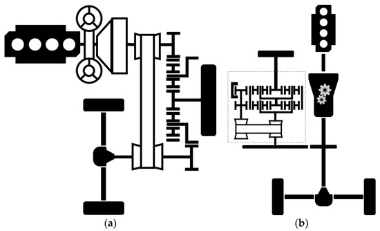
Figure 1.
Flywheel hybrid vehicle schematic with (a) two-degrees-of-freedom [18], and (b) three-degrees-of-freedom [10].
To solve the problems of previous FHV systems, a power-split flywheel hybrid powertrain (PS-FHV) is proposed in this study. The concept of power-splitting is widely used in various hybrid vehicles [20,21]. The concept of power-splitting utilizes a PGS to split the power flow between its three elements: ring gear, sun gear, and carrier. Moreover, from the governing equation of the PGS, it gives additional degrees of freedom to the system [22]. Therefore, the PS-FHV, using a PGS and CVT for its transmission is a 3-DoF system with one active transmission. Since the PS-FHV is 3-DoF FHV system, it is expected to have full hybrid operation modes which makes engine operation as efficient as the HEV. The PS-FHV is expected to have additional mass less than 20 kg, because it uses fewer components than a conventional 3-DoF FHV. From the literature [9], the FESS consists of a flywheel and the additional transmission has a mass of 25 kg, and the PS-FHV uses fewer components than this system. Additionally, PGSs can be fitted into the original transmission and the volume of the FESS is small compared to the motor and battery used in a HEV. Thus, the PS-FHV is compact and light-weight, similar to 2-DoF FHV systems. Overall, the proposed PS-FHV is expected to be a light-weight, compact, and fully-hybridized system, and with further research, it can be commercialized similar to HEV systems.
The remainder of this paper contains the system modeling, various simulations, and analyses to prove that this novel FHV system is feasible and is expected to have good performance. To describe the operational principle of the PS-FHV, its structure is analyzed using the lever analogy. The kinematics and dynamics model of the PS-FHV is analyzed and, using the result, its system DoF and controllability is proven. To estimate the system feasibility and performance, a medium-sized sedan class is used as the target vehicle, and simulations based on the target vehicle are performed. The result of the PS-FHV operation are compared with other vehicle powertrain systems to show that the PS-FHV is a promising flywheel hybrid vehicle system.
2. Lever Analogy and PS-FHV Working Principles
The PS-FHV is a 3-DoF FHV system with two control DoFs. As shown in Figure 2, the ring gear and the sun gear of the three PGSs are connected with each other, the CVT is located between the ring gear of the PGSs, and the engine, the FESS, and the final drive are connected to the carrier of each PGS.
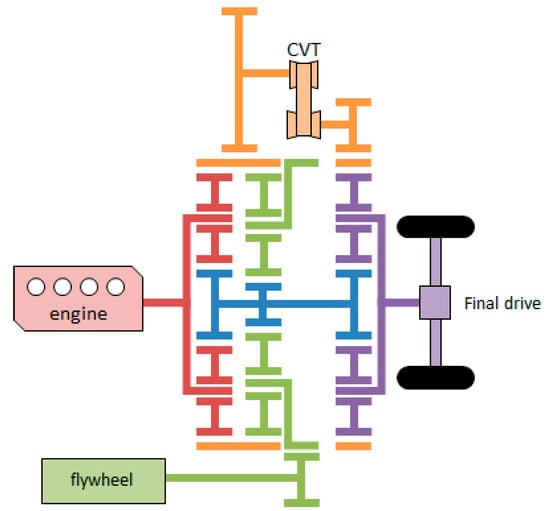
Figure 2.
The PS-FHV configuration, consisting of three PGSs and one CVT.
2.1. The PS-FHV Lever Analogy
To explain the working principles of the PS-FHV, a lever diagram of the PS-FHV system and power analysis can be used. The PGS and CVT are represented by a three-node lever [22,23] and the two PGSs are merged into a four-node lever, as shown in Figure 3. Due to the powertrain configuration, the PS-FHV can be represented by a single lever with six nodes, as shown in Figure 4. Since the CVT can have continuous gear ratios within its operating range, the lever analogy result of the PS-FHV can vary. The lever analogy of the PS-FHV is classified according to its node position, which results in five types of levers, as shown in Figure 5.
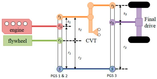
Figure 3.
Lever analogy result of each PGS and CVT in the PS-FHV configuration.
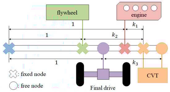
Figure 4.
Single lever expression of the PS-FHV.
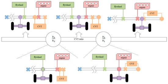
Figure 5.
Changes in node location in the single lever expression of the PS-FHV with change of CVT ratio.
2.2. Working Principles
Changes in the CVT ratio (N) result in changes in the relative position among the lever nodes and involves a torque path change of the PS-FHV. The change in torque transmission path results in a change in the power flow path, resulting driving mode change, as shown in Figure 6 and Figure 7, respectively.
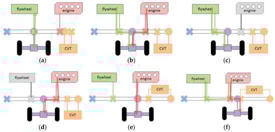
Figure 6.
Power flow path of (a) flywheel drive/engine neutral; (b) assist drive; (c) flywheel drive with engine of; (d) engine drive with flywheel off; (e) engine drive/flywheel neutral; and (f) recharge drive mode.
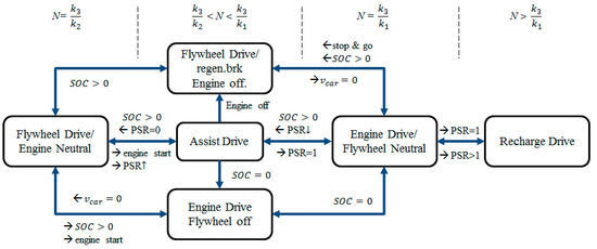
Figure 7.
Operation state diagram of the PS-FHV.
- (1)
- : the FESS node is located between the engine and the final drive. In this case, the engine and final drive node power is transferred to the FESS power, which is not useful for the FHV.
- (2)
- (): the FESS (engine) node and final drive node are at the same point of the lever. In this case, the power of the FESS (engine) is transmitted to the axle, and the engine (FESS) becomes independent from the operation, which is a flywheel drive with a neutral engine (engine drive mode with flywheel neutral).
- (3)
- : the final drive node is between the engine and the FESS. In the assist driving mode, the engine and FESS power are merged into the axle. If the engine or FESS is not operating in this condition, then the system runs in the flywheel drive or engine drive/mode.
- (4)
- : the engine node is between the FESS and the final drive node, i.e., the engine power is divided between the FESS and final drive, representing a recharge driving mode.
3. PS-FHV Modeling
3.1. Kinematics
The PS-FHV uses three PGSs and one CVT; thus, its kinematics derivation process is complex. Based on the lever analogy, the kinematics of each planetary gear used in the PS-FHV is obtained as follows:
Using the CVT kinematics in Equation (4), the engine, FESS, and final drive speed can be substituted for the other angular velocity parameters. As a result, the kinematics of the PS-FHV can be written as follows:
From the speed kinematics equation, the engine speed and the CVT ratio N are the control parameters. The CVT ratio can simultaneously control the engine speed and FESS speed because of the multiple planetary gear connections, resulting in the power regulation control for the engine and the power distribution control between the engine and the FESS. Thus, the PS-FHV is a 3-DoF FHV, capable of full hybrid operation, such as recharge or assist drive mode, with only one active transmission.
3.2. Dynamics
The free body diagram for the dynamic analysis of the PS-FHV is shown in Figure 8 and its torque balance equation is represented in Appendix A. Assuming that the rotational inertia of the gear is small and negligible, the PS-FHV dynamics model of PS-FHV can be derived as follows:
where are the angular acceleration and inertia of the FESS, engine, and final drive, respectively; represent the torque applied to the CVT, engine, and final drive, respectively; and represent the system parameters determined by the sun/ring gear ratio of each PGS, and the CVT ratio. These parameters can be calculated as follows:
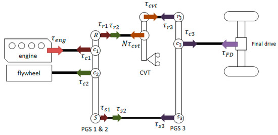
Figure 8.
Free body diagram of the PS-FHV using the lever analogy.
Since are determined by the transmission parameters, changing the PGS ratio of , , and may shift the operation mode and system output ratio.
The three dynamics equations are insufficient to obtain the solution of the entire system, and the control input of the CVT is not shown in the above equation. Therefore, we obtain a new equation through the derivative of the kinematics and group it in the form of a matrix as follows:
In this matrix form, two additional parameters are added: is the rate of change of the CVT ratio N and is its derivative coefficient, which is calculated via the following equation:
In the dynamics equation, the system input is the rate of change in the CVT ratio, engine torque, and load torque in the final drive. Of these, the load torque is a disturbance input, and the remaining two inputs are controllable variables. For the above equation to have a non-trivial solution, the determinant of the inertial matrix in Equation (12) should be non-zero. To simplify, we rewrote the inertial matrix as:
where is the augmented matrix of the inertial terms from Equation (12), and is the augmented 3 1 vector of system parameter equations . The determinant of the matrix in Equation (14) is shown as:
In Equation (15), as , and , the determinant of the inertial matrix in Equation (14) is a non-singular matrix and, therefore, the derived dynamics equation always has a non-zero solution. In physical terms, this means that the speed of the entire system can be controlled by only two control inputs.
The above dynamics equation is used in the whole PS-FHV operation, except for two driving modes: the flywheel drive engine off mode and the engine drive flywheel off mode. In these modes, both speed and acceleration of the FESS or engine is set to zero, and the engine output torque and FESS inertial torque are replaced by the reaction torque of transmission. Thus, the dynamics Equation (12) changes into Equations (16) and (17) for the flywheel drive engine off mode and engine drive flywheel off mode, respectively:
The inertial matrix of Equations (16) and (17) also holds the condition written in Equations (14) and (15), so Equations (16) and (17) have non-trivial solutions. Thus, the two driving modes can be controllable.
For more details of PS-FHV control, system state, control input, and external disturbance are defined and the state control equation is derived. As shown in Table 1, the CVT ratio and the speed of each component are the system states which must be controlled for desired driving; the engine torque and CVT shift speed are the control inputs, and final drive torque is the external disturbance determined by the driving speed and road condition.

Table 1.
State information of the PS-FHV.
Solving Equation (12) for state control, the speed states are controlled by the CVT torque, and current state and configuration parameters are as follows:
Meanwhile, the CVT ratio state N is directly controlled by the CVT shift speed . Thus, each of the four states of the PS-FHV can be controlled. From Equation (12), the CVT torque control equation can be derived as follows:
From Equation (21), the CVT torque can be controlled by every system input, the engine speed, CVT shift speed, and road disturbance, and using the CVT torque, every PS-FHV state can be controlled, as shown in Equations (18)–(20).
Using the control equation result, the control block diagram of PS-FHV is shown in Figure 9. The driver input determines the CVT torque reference and a high level controller determines the system control inputs for desired operation, such as the economic driving mode. This control input reference goes to each controller and the generated control input controls the four PS-FHV states. These four states are used to generate the control inputs and, among the four PS-FHV states, the final drive speed becomes the vehicle output speed.
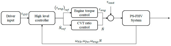
Figure 9.
The PS-FHV control block diagram.
4. Simulation of the PS-FHV
4.1. Simulation Settings
Based on the previous powertrain modeling, simulations were conducted to evaluate the system feasibility, acceleration performance, and fuel efficiency. To evaluate the PS-FHV feasibility, gradeability and drivability were analyzed using the transmission torque curve of the target PS-FHV. For the evaluation of the acceleration performance, 0–100 km/h time and 0–160 km/h time were calculated using a full-acceleration driving simulation. For the fuel economy performance of PS-FHV, the urban dynamometer driving schedule (UDDS) and the highway fuel economy test (HWFET) drive cycle simulations were conducted based on the instantaneous optimization of the driving point.
The target vehicle in the simulation was based on a medium-sized sedan-class vehicle [24,25]. For the transmissions, the planetary gear ratios were set to enable all required hybrid operations within the range of typical CVT ratios [26] and the efficiency of transmission element was set as 98% for the PGSs and the CVT, as shown Figure 10. A final drive reduction gear and a flywheel reduction gear were added to match the system operating speed range. For the engine, a 120-kW engine with an output similar to that of a typical mid-sized sedan was used [24]. The torque-speed diagram of the engine and the brake specific fuel consumption (BSFC) map are shown in Figure 11. The FESS in the simulation was obtained from a previous FHV study [11]. The spin loss of the FESS, which is one of the important elements of a FESS, is shown in Figure 12. The other parameters are shown in Table 2.
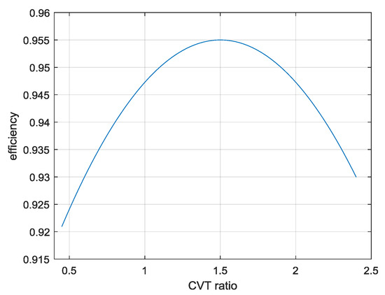
Figure 10.
CVT efficiency profile with respect to the CVT ratio [20].
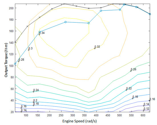
Figure 11.
The speed-torque curve of the maximum output engine model (represented by points marked with an “x”), and the efficiency and optimal operating point (represented by points marked with an “o”).
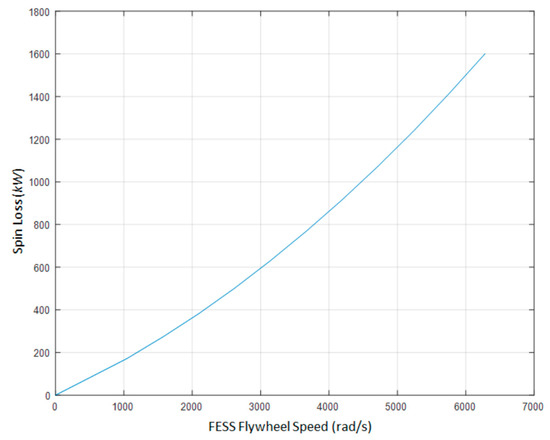
Figure 12.
FESS spin loss versus flywheel speed [11].
Table 2.
The parameter setup for the PS-FHV simulation.
For the simulation, the following assumptions were made to reduce the calculation load and simulation complexity.
Assumption 1.
The tire dynamics are neglected.
Tire dynamics are important not only with respect to lateral movement, but also in the longitudinal movement of a vehicle. However, tire dynamics are difficult to model and the driving simulation is less dynamic than the rapid braking simulation. Therefore, tire dynamics are neglected in the driving simulation.
Assumption 2.
The PGS efficiency is 98%.
The PGS reference efficiency map in previous transmission research shows a low level of change in the PGS efficiency with respect to the gear ratio and power. Thus, for calculation convenience, PGS efficiency is assumed to be constant. Since, there are no additional components in the PS-FHV PGS, while an automatic transmission requires a hydraulic circuit for the clutch operation in its PGS, the constant value is set to 98%.
Assumption 3.
The auxiliary power is 700 W.
There are many auxiliaries in vehicle systems, such as the air conditioning system and the vacuum pump for braking, among others. Some of these systems are essential for vehicle driving. Thus, the auxiliary power demand for vehicle driving is assumed to be constant and the value is fixed to 700 W.
Assumption 4.
The torque and speed demand for the next step in the driving cycle simulation is known.
For the driving cycle simulation, there are two methods to derive the control input that gives the desired output: forward and backward calculation. The forward calculation, which is a causal method, calculates vehicle output among the various control inputs and finds the best output suitable for the demand. The backward calculation, the non-causal method, finds the control output that meets the vehicle demand and selects among the solutions. Each method has advantages, but as the backward calculation has a lower calculation load and no output error, the backward calculation method is used for the driving cycle simulation.
Assumption 5.
The dynamics of engine starter motor is fast enough so it is neglected in simulations.
To start the engine, an engine starter motor gives initial rotational torque to the engine. This engine starter motor has fast dynamics compared to other vehicle dynamic system, so the dynamics of the engine starter motor are neglected. As a result, starting the engine is considered to be instant.
4.2. Transmission Speed-Torque Curve
The transmission torque curve was obtained and used for the feasibility assessment. To obtain the static output torque with respect to vehicle speed, both the kinematics and dynamics models were used.
From the PS-FHV kinematics, the speed relationships among the final drive, engine, and FESS were determined by three PGSs and a CVT. As we add reduction gears in the simulation of the PS-FHV transmission model, the kinematic equation changes into the following equation:
From Equation (22), the final drive speed is related to the FESS speed, and the FESS state of charge (SOC) is a function of its speed. Therefore, unlike the transmission torque curve of conventional vehicles, the PS-FHV transmission torque is dependent on the FESS SOC.
The output torque of the PS-FHV can be obtained from Equation (12). When the acceleration of the engine and the final drive are zero, all the engine output is used to overcome the load torque, and the PS-FHV has maximum output. In this situation, the matrix in Equation (12) changes into the following equations:
From the equations above, the transmission output torque is determined by the engine torque and the FESS inertial torque, and the inertial torque is determined by the CVT shift speed. As the inertial torque has no limitation, the transmission output torque is determined by the engine maximum torque and the CVT shift speed.
In the assist drive mode and the recharge drive mode, the CVT torque is redundant to both the engine and the flywheel. Therefore, the transmission output torque is determined by the minimum engine and the maximum FESS output torque, as shown in Equation (26). In the engine drive mode and the flywheel drive mode, the maximum engine torque and FESS inertial torque, derived using Equation (24), determines the transmission output torque. Therefore, the maximum transmission output torque is the maximum transmission torque among the four drive modes, as shown in Equation (27).
Using Equation (27), the transmission torque map of the entire powertrain with respect to the FESS SOC can be derived, as shown in Figure 13:
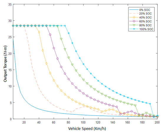
Figure 13.
PS-FHV speed-torque curve versus vehicle speed and FESS SOC status.
Figure 14 shows that the usage of the FESS can be determined according to the vehicle speed and the FESS SOC. When the SOC of the FESS is relatively higher than the vehicle speed, the CVT can adjust its ratio for the flywheel drive mode. In high-vehicle-speed situations, the CVT ratio cannot match the FESS speed because the flywheel speed is relatively lower than the vehicle speed. Thus, the maximum torque is generated in the assist drive mode instead of the flywheel drive mode, and the engine adds additional power to the vehicle.
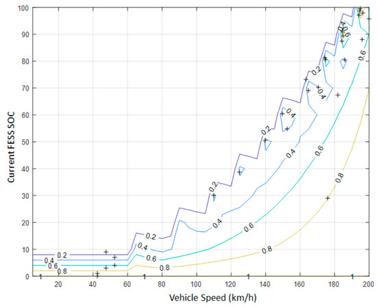
Figure 14.
PS-FHV PSR ratio at maximum driving torque.
4.3. Feasibility Assessment and Acceleration Performance
To determine whether the power-split vehicle is feasible, drivability and gradeability tests were conducted. Drivability is defined as the highest speed that the vehicle can reach, and gradeability is defined as the highest grade that the vehicle can ascend. Both drivability and gradeability are related to the load torque to the vehicle, which can be calculated using Equation (28):
where the road load consists of rolling friction and aerodynamic resistance, and the gradient resistance used for the gradeability test [27]. The equation for the driving road load is as follows:
The calculated result for the load torque is shown in Figure 15. With the transmission torque map from Figure 14, the maximum drivability of the target PS-FHV with respect to the incline can be calculated. Under a zero-inclination condition, the target PS-FHV can drive up to 220 km/h. Assuming that the minimum ascending speed for the target vehicle is 15 km/h, the minimum gradeability for the PS-FHP is 40%.
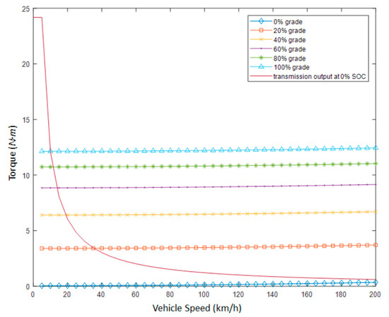
Figure 15.
Target vehicle load torque profile with PS-FHV output at 0% SOC status.
To estimate the acceleration performance of the target PS-FHV, the 0–100 km/h time and the 0–160 km/h time were calculated using the full-acceleration simulation. To obtain maximum torque with respect to vehicle speed, the transmission speed torque curve was used and the 0% inclination load torque was used. Since the output torque of the PS-FHV was different with respect to the FESS SOC, acceleration resulted in changes with respect to the initial SOC, as shown in Figure 16. In Figure 16, the PS-FHV driving begins with the flywheel drive, if possible, and shifts to assist drive until the FESS is depleted. Since the FESS SOC status determines the duration of the flywheel drive mode, which produces the highest output torque, a higher initial SOC results in better acceleration performance. For the zero initial SOC case, the vehicle has no time to charge and use its FESS; therefore, driving occurs in the engine-only drive mode. Using the acceleration simulation result, the 0–100 km/h time and the 0–160 km/h time with respect to the FESS SOC were derived, as shown in Figure 17.
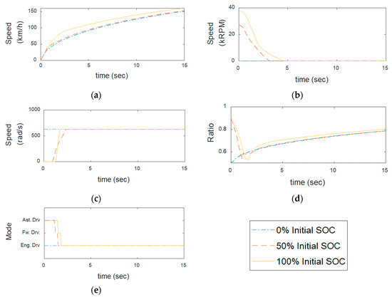
Figure 16.
Acceleration simulation result plot at 0%, 50%, and 100% initial SOC: (a) vehicle speed profile; (b) flywheel speed profile; (c) engine speed profile; (d) CVT Ratio Profile; and (e) driving mode profile.
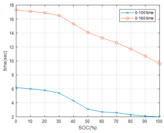
Figure 17.
The 0–100 km/h time and 0–160 km/h time result versus initial SOC.
4.4. Fuel Economy
The PS-FHV fuel economy of the PS-FHV was predicted via the target vehicle driving cycle simulation of the target vehicle. The driving cycles used in this simulation are the UDDS cycle and HWFET cycle, which represent urban driving and highway driving, respectively.
The simulation was performed based on an equivalent consumption management simulation (ECMS), which is an instantaneous optimization method often used in simulations of electric hybrid cars [28,29]. In the ECMS simulation, the engine and CVT operation point were selected to minimize the following equation:
where is the engine fuel consumption ratio, specified in Figure 11, and is a coefficient factor. To calculate the operating point and its corresponding fuel consumption ratio, the power demand of the vehicle is calculated as follows:
Using the speed and torque demand of the vehicle, the required engine and torque can be derived using the following equations:
In the assist mode or the recharge drive mode, FESS power and CVT shift speed are automatically calculated using Equation (12). However, in the flywheel drive and regenerative braking modes, the engine does not operate, so Equations (37) and (38) do not hold. In these cases, the FESS supplies or takes every power demand to or from the vehicle. Thus, using Equation (39), the FESS power and the corresponding CVT shift speed can be calculated:
Using the above equations, the instantaneous optimization of the UDDS and HWFET driving cycle simulations is achieved. To determine the fuel economy, a driving simulation was performed under the SOC sustained condition. Figure 18 and Figure 19 show the results of running the simulation for two driving cycles, displaying the speed profile, operation modes, CVT ratio, and shifting speed.
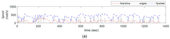

Figure 18.
PS-FHV UDDS drive cycle result: (a) speed profile; (b) power profile; (c) driving mode profile; and (d) CVT ratio and shift speed profile.
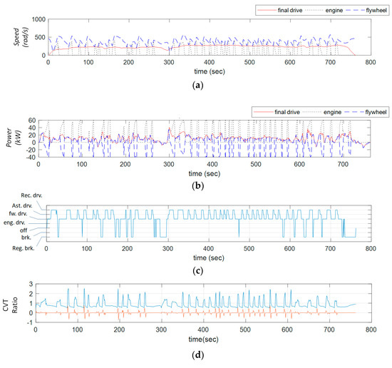
Figure 19.
PS-FHV HWFET drive cycle result: (a) speed profile; (b) power profile; (c) driving mode profile; and (d) CVT ratio and shift speed profile.
From the simulation results, the PS-FHV has two kinds of driving characteristics. First, the FESS saves energy while the vehicle is braking and uses the saved energy in acceleration, which can be seen in the 200–400 s region in Figure 18. This driving characteristic can be seen in other hybrids, because the energy stored by regenerative braking used in acceleration is a key in the operation of hybrid vehicles. The second driving characteristic is that the PS-FHV constantly switches the operation between the flywheel drive and the recharge drive mode while the vehicle is constantly demanding power. This operation characteristic can be seen at the 300–400 s region in Figure 19. Here, the flywheel repeats charging and discharging while the vehicle speed is almost constant. This mode switching characteristics cannot be seen in other hybrids (such as parallel HEVs and power-split HEVs), but can be explained using series HEV operation. In series HEV, the engine always operates on the most efficient operating point to generate electrical power and the motor uses this power to generate vehicle power demand. Since the FESS has no conversion loss and can afford unlimited power to the vehicle, it efficiently operates by using the engine to charge the FESS and drives using the charged FESS. The spin loss of the FESS increases when the FESS has a high SOC, but operating the engine at the most efficient position is much more efficient even with the high FESS spin loss.
The switching drive mode characteristics affect the engine operating point and the relationship between the flywheel speed and vehicle speed. In Figure 20, the engine operation is at the most efficient operating point, even when the vehicle power demand is low. In Figure 21, not only an arch-shape profile, but also the vertical line can be seen in both drive cycle simulations. The arch-shape profile is due to regenerative braking and the flywheel drive operating under an acceleration condition. The vertical line in both Figure 21a,b denotes that the flywheel speed constantly changes with small vehicle speed changes, which is caused by the PS-FHV switching operation. Since the HWFET drive cycle features a more constant driving speed than the UDDS driving cycle, more vertical lines can be observed in Figure 21b than in Figure 21a.
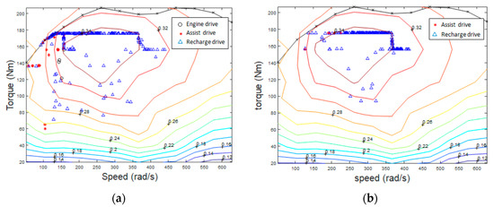
Figure 20.
Engine operating point: (a) UDDS driving cycle simulation; and (b) HWFET driving cycle simulation.
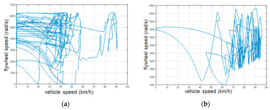
Figure 21.
FESS speed versus vehicle speed: (a) UDDS driving cycle; and (b) HWFET driving cycle.
Figure 21 also shows that no constraints were found between FESS and vehicle speed. In Figure 21a, the FESS speed can be non-zero when the vehicle is stopped because the PS-FHV has a driving mode called FESS neutral mode, which separates the FESS and the vehicle. The CVT operation and the shifting speed profile in the PS-FHV driving simulation showed that the CVT stays mostly near 0.9, due to frequent driving mode shifts. In the flywheel drive mode, the CVT ratio drops to 0.5 and then increases to operate in the recharge driving mode. In the recharge drive mode, the CVT ratio increases up to 2.5, which is the maximum CVT ratio, because the higher the CVT ratio, the more engine power is directed to the FESS. The fuel economy resulting from both driving cycles are shown in Table 3.
Table 3.
Drive cycle simulation results.
To observe the power flow between the engine, transmission, and FESS in the drive cycle simulation, an energy analysis was performed. From Figure 22, during the driving condition, approximately 60–70% of the power produced by the engine was used by the vehicle, and the other 10–15% was used to charge the FESS. During the braking condition, approximately 38% of the braking power from the vehicle was converted to FESS charge. From the engine perspective, approximately 30% of the power from fuel was converted to mechanical energy, as shown in Figure 23, and distributed to the vehicle and the FESS with some loss, as shown in Figure 23. Conversely, the FESS lost its energy due to spin loss, flywheel driving, and assist driving, and gained energy from the engine and the vehicle by recharge driving and regenerative braking, respectively. As shown in Figure 24, the FESS was mostly discharged by the flywheel drive mode, and was mostly charged by the recharge drive mode.
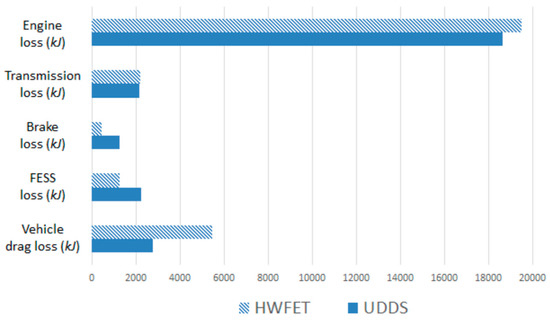
Figure 22.
Energy loss analysis result for driving cycle simulations from the vehicle perspective.
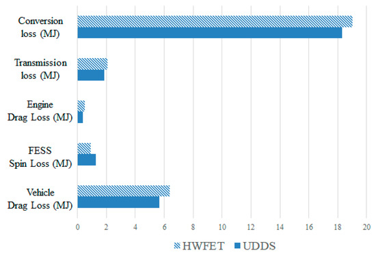
Figure 23.
The loss analysis of fuel energy in driving cycle simulations.

Figure 24.
FESS energy input and output analysis in drive cycle simulations.
4.5. Comparative Study
To determine the competitiveness of the PS-FHV, the simulation results of the PS-FHV were compared with other commercial powertrains: a manual transmission (MT) vehicle, a parallel HEV (PHEV), and a power-split HEV (PS-HEV). For the driving cycle simulation for fuel economy performance, an ECMS simulation, the same as for the PS-FHV driving cycle, was conducted. For the acceleration simulation, Advisor (the MATLAB vehicle drive simulation tool developed by the National Renewable Energy Lab (NREL), Golden, CO, USA) was used [30]. Since Advisor is a simulation tool used in HEV research [24,29,31], and commercial HEV specifications [32] show similar performance as the Advisor simulation results presented below, using Advisor as a comparison tool is reasonable. The comparison vehicles are modeled using previous studies and the parameters, such as mass and output power, are adjusted to be similar to the PS-FHV as shown in Appendix B. Based on this system setup, the fuel economy of both the UDDS and HWFET drive cycles, and acceleration performance, such as the 0–100 km/h time and the 60–120 km/h time, were simulated and compared with those of the PS-FHV.
The simulation results of the other vehicles are shown in Figure 25. Figure 25 shows that the PHEV and the PS-HEV had fuel economy improvements, but acceleration was similar to the conventional vehicle.
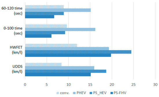
Figure 25.
PS-FHV performance estimation versus other vehicle types.
Specifically, the PS-FHV operates its engine more efficiently than the PHEV and a conventional vehicle, but is less efficient than a PS-HEV. From Figure 26, PS-FHV had more energy loss in the UDDS and HWFET driving cycles than other HEV systems in terms of the energy storage system (ESS) and the transmission. The reason for the greater loss is because the FESS has significant flywheel spin loss compared to the battery, and the PS-FHV uses more mechanical transmission components than does a PHEV or a PS-HEV. However, due to the proposed PS-FHV PGS+CVT transmission, the engine operating point is more optimized than that for the PHEV
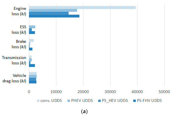
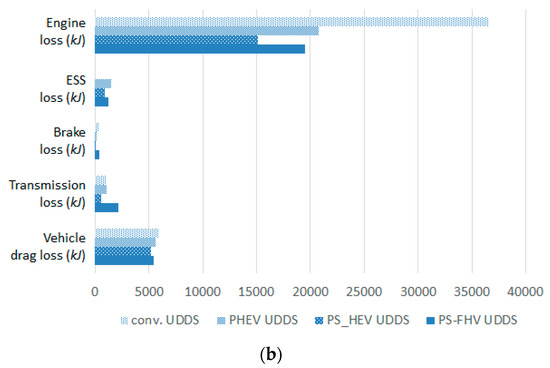
Figure 26.
Comparing energy loss between the PS-FHV and other powertrain types; (a) UDDS driving cycle; and (b) HWFET driving cycle.
To clearly compare the simulation results, a radar chart was used to show the performance improvement over the conventional vehicle, as shown in Figure 27. From the radar chart, the PS-FHV has the best acceleration performance, with an improvement of approximately 42%, and is less efficient than the PS-HEV, but similar to the PHEV. In conclusion, the PS-HEV is expected to be a good hybrid powertrain due to its superior acceleration performance and moderate fuel economy (falling between the two existing HEV systems).
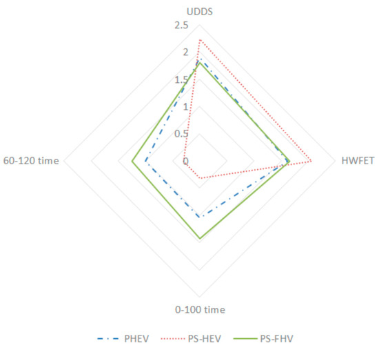
Figure 27.
Performance comparison of the proposed flywheel hybrid powertrain with other powertrain types.
5. Conclusions
In this study, a PS-FHV with three PGSs and one CVT was proposed. The system has 3-DoF with two control DoF because of a CVT and the 2-DoF characteristics of the PGSs. The working principle of the PS-FHV is analyzed using a lever analogy. Kinematics and dynamics modeling of the PS-FHV were conducted to show that the system has three DoF and is controllable. As a result, the PS-FHV provides a hybrid driving mode in any desired operational state. To assess the feasibility and predict PS-FHV performance, various simulations were performed. The gradeability and drivability were tested using a transmission torque map, and the acceleration and fuel economy performance were estimated using a transmission torque map and a drive cycle simulation. In the simulations, the PS-FHV was able to accelerate up to 200 km/h and overcome a grade of at least 45%. To estimate the PS-FHV performance compared with that of other vehicles, a conventional vehicle, a PHEV, and a PS-HEV were simulated using Advisor. The comparison results showed that compare to the other two HEVs, the PS-FHV had the best acceleration performance and a similar fuel economy. As a result, the proposed flywheel hybrid system is expected to be a competitive hybrid powertrain.
For the next step of the research, an analysis of the physical PGS+CVT design space within the PS-FHV, and finding the optimal configuration of the PS-FHV, are being studied to realize an actual PS-FHV and pursue further production.
Author Contributions
Conceptualization: C.S.; formal analysis: C.S.; methodology: C.S.; writing—original draft: C.S.; and writing—review and editing: D.K. and K.-S.K.
Funding
This research was supported by BK21 Plus Program. This research was also supported by a grant (17TLRP-C135446-01, Development of Hybrid Electric Vehicle Conversion Kit for Diesel Delivery Trucks and its Commercialization for Parcel Services) from Transportation & Logistics Research Program (TLRP) funded by Ministry of Land, Infrastructure and Transport of Korean government.
Conflicts of Interest
The authors declare no conflict of interest.
Appendix A
In these equations, we substitute , , and , the torque terms of each node, and rewrite the equations based on the speed of the engine, flywheel, and final drive and the torque applied to the CVT. The overall dynamics model are summarized by Equations (6)–(8) in Section 3.2
Appendix B
Table A1.
Parameters of comparison vehicles: conventional, PHEV, and PS-HEV.
Table A1.
Parameters of comparison vehicles: conventional, PHEV, and PS-HEV.
| Variable Name | Value | |
|---|---|---|
| Conventional vehicle | Transmission mass | 114 kg |
| Transmission ratios | 1st gear: 3.57 | |
| 2nd gear: 2 | ||
| 3rd gear: 1.33 | ||
| 4th gear: 1 | ||
| 5th gear 0.75 | ||
| Final drive ratio | 3.77 | |
| Transmission efficiency | 92% | |
| PHEV vehicle | Motor mass | 60 kg |
| Motor power | 49 kW | |
| Battery mass | 210 | |
| Battery max power | 50 kW | |
| PS-HEV vehicle | Motor mass | 57 |
| Motor power | 30 kW | |
| Generator mass | 33 | |
| Generator power | 15 kW | |
| Battery mass | 138 | |
| Battery power | 51 kW |
Vehicle mass is the same for four types of vehicles. PHEV uses the same transmission as the conventional vehicle.
References
- Chan, C.C. The State of the Art of Electric, Hybrid, and Fuel Cell Vehicles. Proc. IEEE 2007, 95, 704–718. [Google Scholar] [CrossRef]
- Baseley, S.; Ehret, C.; Greif, E.; Kliffken, M.G. Hydraulic Hybrid Systems for Commercial Vehicles; SAE International: Warrendale, PA, USA, 2007. [Google Scholar]
- Hebner, R.; Beno, J. Applications Ranging from Railroad Trains to Space Stations. IEEE Spectr. 2002, 39, 46–51. [Google Scholar] [CrossRef]
- Lukic, S.M.; Cao, J.; Bansal, R.C.; Rodriguez, F.; Emadi, A. Energy Storage Systems for Automotive Applications. IEEE Trans. Ind. Electron. 2008, 55, 2258–2267. [Google Scholar] [CrossRef]
- Ibrahim, H.; Ilinca, A.; Perron, J. Energy storage systems—Characteristics and comparisons. Renew. Sustain. Energy Rev. 2008, 12, 1221–1250. [Google Scholar] [CrossRef]
- Kapoor, R.; Parveen, C.M. Comparative study on various KERS. In Proceedings of the World Congress on Engineering, London, UK, 3–5 July 2013. [Google Scholar]
- Bolund, B.; Bernhoff, H.; Leijon, M. Flywheel Energy and Power Storage Systems. Renew. Sustain. Energy Rev. 2007, 11, 235–258. [Google Scholar] [CrossRef]
- Dhand, A.; Pullen, K. Review of Flywheel Based Internal Combustion Engine Hybrid Vehicles. Int. J. Automot. Technol. 2013, 14, 797–804. [Google Scholar] [CrossRef]
- Hansen, J.G. An Assessment of Flywheel High Power Energy Storage Technology for Hybrid Vehicles; Oak Ridge National Laboratory (ORNL): Oak Ridge, TN, USA, 2011. [Google Scholar]
- Diego-Ayala, U.; Martinez-Gonzalez, P.; McGlashan, N.; Pullen, K.R. The Mechanical Hybrid Vehicle: An Investigation of a Flywheel-Based Vehicular Regenerative Energy Capture System. Proc. Inst. Mech. Eng. Part D J. Automob. Eng. 2008, 222, 2087–2101. [Google Scholar] [CrossRef]
- Cross, D.; Brockbank, C. Mechanical Hybrid System Comprising a Flywheel and CVT for Motorsport and Mainstream Automotive Applications; SAE International: Warrendale, PA, USA, 2009. [Google Scholar]
- Armbruster, D.; Hennings, S. Porsche GT3 R Hybrid Prototype and Race Lab. ATZautotechnology 2011, 11, 12–17. [Google Scholar] [CrossRef]
- Schilke, N.A.; Dehart, A.O.; Hewko, L.O.; Matthews, C.C.; Pozniak, D.J.; Rohde, S.M. The Design of an Engine-Flywheel Hybrid Drive System for a Passenger Car; SAE International: Warrendale, PA, USA, 1984. [Google Scholar]
- Schilke, N.A.; DeHart, A.O.; Hewko, L.O.; Matthews, C.C.; Pozniak, D.J.; Rohde, S.M. The Design of an Engine-Flywheel Hybrid Drive System for a Passenger Car. Proc. Inst. Mech. Eng. Part D Transp. Eng. 1986, 200, 231–248. [Google Scholar] [CrossRef]
- Van Berkel, K.; Hofman, T.; Vroemen, B.; Steinbuch, M. Optimal Control of a Mechanical Hybrid Powertrain. IEEE Trans. Veh. Technol. 2012, 61, 485–497. [Google Scholar] [CrossRef]
- Shen, S.; Veldpaus, F.E. Analysis and Control of a Flywheel Hybrid Vehicular Powertrain. IEEE Trans. Control Syst. Technol. 2004, 12, 645–660. [Google Scholar] [CrossRef]
- Shen, S.; Serrarens, A.; Steinbuch, M.; Veldpaus, F. Coordinated Control of a Mechanical Hybrid Driveline with a Continuously Variable Transmission. JSAE Rev. 2001, 22, 453–461. [Google Scholar] [CrossRef]
- Van Druten, R.M. Transmission Design of the Zero Inertia Powertrain; Technische Universiteit Eindhoven: Eindhoven, The Netherlands, 2001. [Google Scholar]
- Son, H.; Park, K.; Hwang, S.; Kim, H. Design Methodology of a Power Split Type Plug-In Hybrid Electric Vehicle Considering Drivetrain Losses. Energies 2017, 10, 437. [Google Scholar] [CrossRef]
- Cheong, K.L.; Li, P.Y.; Chase, T.R. Optimal Design of Power-Split Transmissions for Hydraulic Hybrid Passenger Vehicles. In Proceedings of the 2011 American Control Conference, San Francisco, CA, USA, 29 June–1 July 2011. [Google Scholar]
- Van Druten, R.M.; van Tilborg, P.G.; Rosielle, P.C.J.N.; Schouten, M.J.W. Design and Constriction Aspects of a Zero Inertia CVT for Passenger Cars II—Design and Constriution Aspects of a Zero Inertia CVT for Passenger Cars. Int. J. Automot. Technol. 2000, 1, 42–47. [Google Scholar]
- Benford, H.L.; Leising, M.B. The Lever Analogy: A New Tool in Transmission Analysis; SAE International: Warrendale, PA, USA, 1981. [Google Scholar]
- Mahoney, J.E.; Maguire, J.M.; Bai, S. Ratio Changing the Continuously Variable Transmission; SAE International: Warrendale, PA, USA, 2004. [Google Scholar]
- Kim, S.J.; Kim, K.-S.; Kum, D. Feasibility Assessment and Design Optimization of a Clutchless Multimode Parallel Hybrid Electric Powertrain. IEEE/ASME Trans. Mechatron. 2016, 21, 774–786. [Google Scholar] [CrossRef]
- Kim, S.J.; Song, C.; Kim, K.-S.; Yoon, Y.-S. Analysis of the Shifting Behavior of a Novel Clutchless Geared Smart Transmission. Int. J. Automot. Technol. 2014, 15, 125–134. [Google Scholar] [CrossRef]
- Ruan, J.; Zhang, N.; Walker, P. Comparing of Single Reduction and CVT Based Transmissions on Battery Electric Vehicle. In Proceedings of the 14th IFToMM World Congress in Mechanism and Machine Science, Taipei, Taiwan, 25–30 October 2015; pp. 610–618. [Google Scholar]
- Yamsani, A. Gradeability for Automobiles. IOSR J. Mech. Civ. Eng. 2014, 11, 35–41. [Google Scholar] [CrossRef]
- Paganelli, G.; Delprat, S.; Guerra, T.M.; Rimaux, J.; Santin, J.J. Equivalent Consumption Minimization Strategy for Parallel Hybrid Powertrains. IEEE Veh. Technol. Conf. 2002, 4, 2076–2081. [Google Scholar]
- Sciarretta, A.; Back, M.; Guzzella, L. Optimal Control of Parallel Hybrid Electric Vehicles. IEEE Trans. Control Syst. Technol. 2004, 12, 352–363. [Google Scholar] [CrossRef]
- Markel, T.; Brooker, A.; Hendricks, T.; Johnson, V.; Kelly, K.; Kramer, B.; O’Keefe, M.; Sprik, S.; Wipke, K. ADVISOR: A Systems Analysis Tool for Advanced Vehicle Modelling. J. Power Sources 2002, 110, 255–266. [Google Scholar] [CrossRef]
- Wipke, K.B.; Cuddy, M.R.; Burch, S.D. ADVISOR 2.1: A User-Friendly Advanced Powertrain Simulation Using a Combined Backward/Forward Approach. IEEE Trans. Veh. Technol. 1999, 48, 1751–1761. [Google Scholar] [CrossRef]
- 2018 Toyota Camry MPG & Price. Available online: https://www.toyota.com/camry/features/mpg/2559/2561/2560 (accessed on 13 May 2018).
© 2018 by the authors. Licensee MDPI, Basel, Switzerland. This article is an open access article distributed under the terms and conditions of the Creative Commons Attribution (CC BY) license (http://creativecommons.org/licenses/by/4.0/).