Analysis of Ferroresonance Phenomenon in 22 kV Distribution System with a Photovoltaic Source by PSCAD/EMTDC

Abstract

Overvoltage and overcurrent in the middle voltage (MV) 22 kV and low voltage (LV) 0.4 kV distribution network with photovoltaic (PV) rooftop system of the Provincial Electricity Authority of Thailand (PEA) have been investigated in order to show that these unwanted situations are caused by the ferroresonance phenomenon. This information would be useful to improve a better solution for the system protection when PV rooftops are integrated into the PEA distribution system. The software tool, PSCAD/EMTDC is used to study the overvoltage at the high side of open-delta and open-wye distribution transformer- and overcurrent at the low side of distribution transformer linked to the grid system via three single-phase fuse cutouts. The ferroresonance phenomenon can be observed when the PV rooftop system is linked to the low voltage side of the distribution transformer via three single-phase fuse cutouts. The results show a good similarity with the results from the simulation of the MV side and LV side of distribution transformers. Finally, the physical phenomena described to the overvoltage, overcurrent, and the destruction of the distribution transformer and other apparatus in load customers will occur when the system consists of the PV rooftop source, capacitance in long transmission line, nonlinear distribution transformer with saturation characteristic and the usage of single-phase switching cutouts in the system.

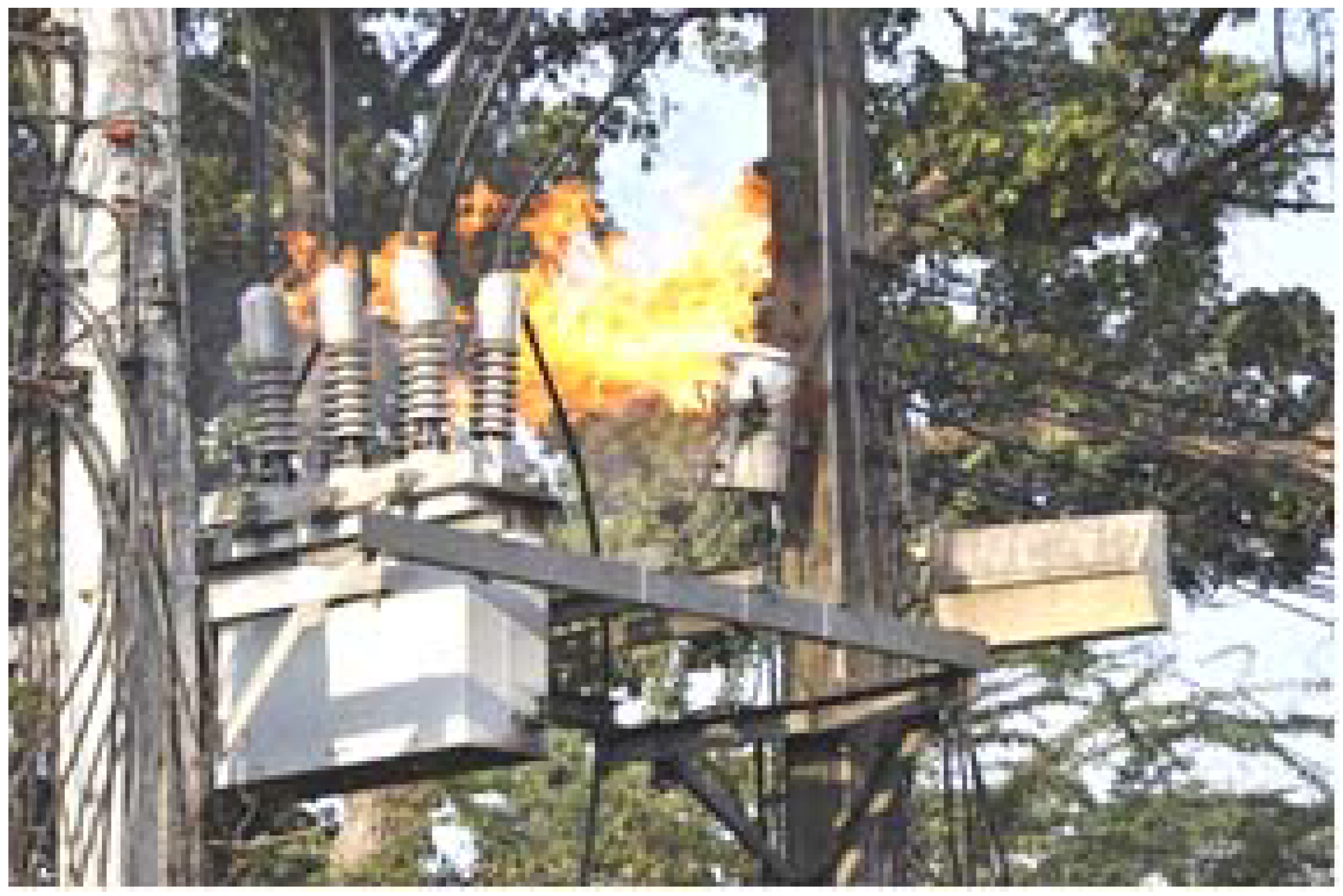
1. Introduction

Ferroresonance is a special kind of resonance that occurs in the network with nonlinear elements, especially in transformers. When nonlinear inductance of the transformer core and the capacitance of the network are equal, ferroresonance happens. This equality can occur when the transformer is accidentally energized and de-energized in only one or two phases. Ferroresonance results in a high current and voltage across the inductance core and leads to the damage of the transformer as shown in Figure 1. There are a lot of articles in the literature which have discussed this phenomenon, for instance, References [1,2,3,4,5,6,7,8], and numerous simulation results of the possible ferroresonance happening in the high voltage side of the distribution network have been reported in References [9,10,11,12]. Gonen T. reported that ferroresonance is a transient phenomenon caused by the interaction of system capacitance with the nonlinear inductance of the transformer, energy source, and limited power losses [13]. However, Garikoitz B., et al. showed that the influence of ferroresonance is not only limited to the cable capacitance consideration, but also to several constructive, design, operation, and protective parameters [14]. There are a lot of ferroresonances in the configuration of distribution transformers. In 2003, Jacobson D.A.N. determined that seven different types of electrical systems are affected by ferroresonance phenomena [15].

This phenomenon has been considered and concentrated by the large-scale electricity generators that produce and distribute energy to the end user. Nowadays, electricity is not only produced by large-scale producers but also by the small-scale end users. The development of the electricity generation technology and energy policies together with the environmental crisis have persuaded the end users to produce electricity from renewable energy by themselves. Therefore, ferroresonance caused by energizing and de-energizing transformers which are connected to these small-scale electricity producers must be of concern.

One of the small-scale electricity generation systems from renewable energy is the photovoltaic (PV) system, which directly converts solar energy into electricity. It is one of the significant and clean sources of renewable energy. In the year 2012, Thailand has successfully installed nearly 2300 MW of solar energy, 99 percent of which is in the form of commercially centralized installations (solar farms), while the housing-sized solar PV (solar rooftop) shares a very small percentage [17,18]. However, according to the explosive growth of urbanization in Thailand, which increases every year (approximately 1.6 percent per year [17]), the usage of rooftop solar energy dramatically increased. In contrast with this growth, the information about the end users that can produce electricity is not fully known by the provincial electricity authority of Thailand (PEA), which is the main electricity distributor in Thailand. Therefore, ferroresonance phenomena from accidentally energizing and de-energizing the distribution transformer should be awarded and concentrated. The study in Reference [19] confirmed that ferroresonance does exist in the power transformer, which is connected to the PV system. However, the complete distribution network is not considered. Moreover, the analysis of the ferroresonance effect on the load is still not considered. With more information on ferroresonance in distribution systems with PV systems connected to it, the PEA will be aware of the effect of this phenomenon on the transformers and the power qualities [20,21,22,23,24,25,26,27,28,29].

Based on these facts, the simulation-based study of the ferroresonance effects in the distribution network with PV system sources will be presented in this paper. The major contribution of this work is the analysis of the type of ferroresonance that occurs in systems together with its effect on the system. The frequency analysis technique known as the Fast Furrier Transformation (FFT) will be used to distinguish the type of ferroresonance in the frequency domain. After the introduction in the first part, the organization of this paper is arranged in 4 parts. In the second part, the preliminary and Theory of ferroresonance will be presented. System modeling and the simulation results will be mentioned, analyzed and discussed in the third and fourth part, respectively. Finally, the conclusion will be addressed in the last part.

2. Preliminary and Theory

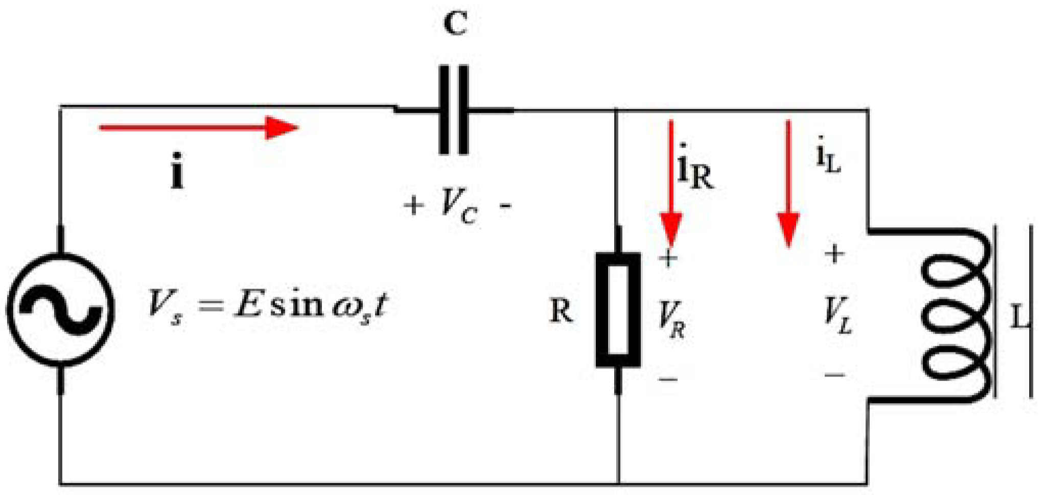
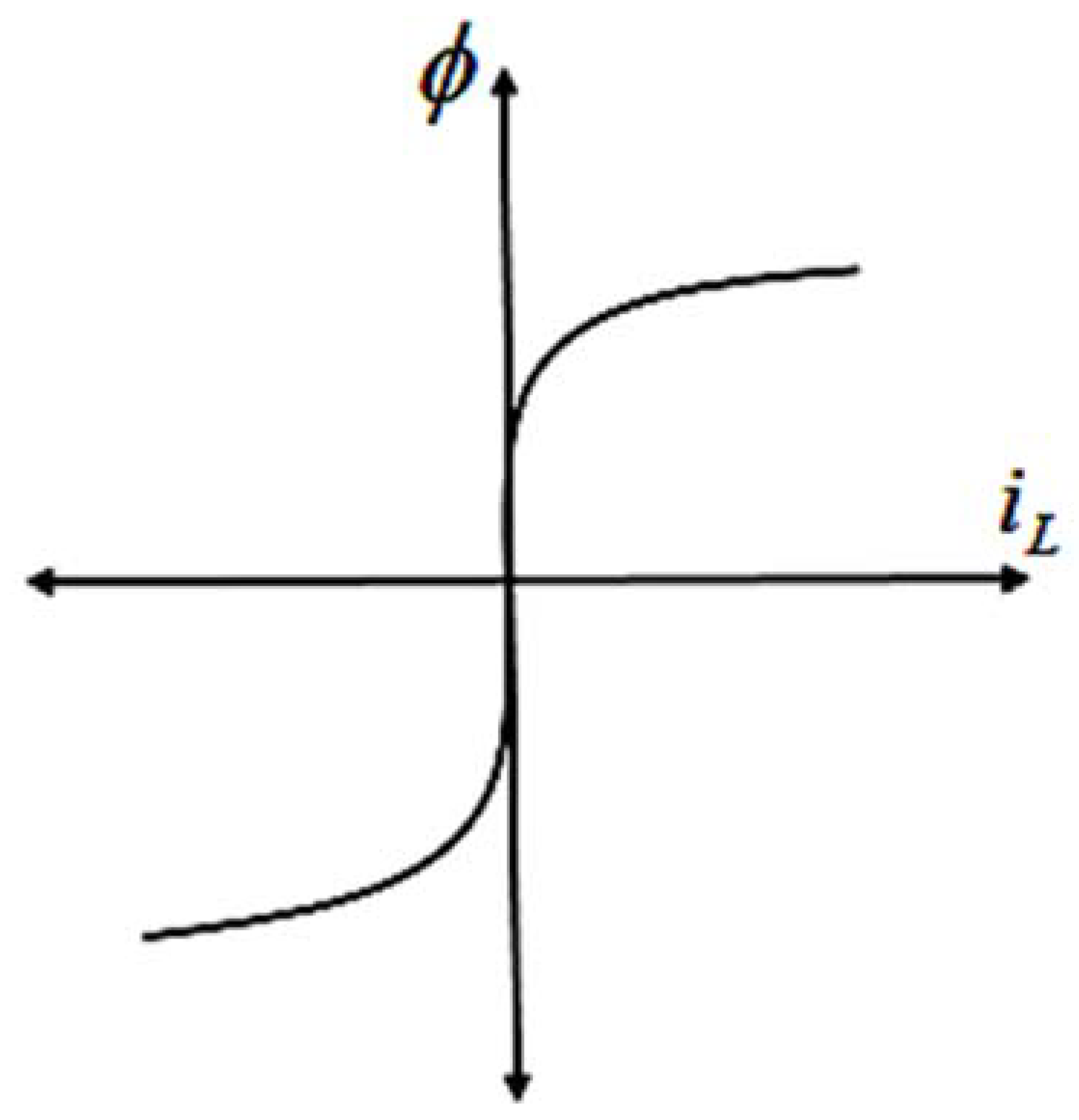
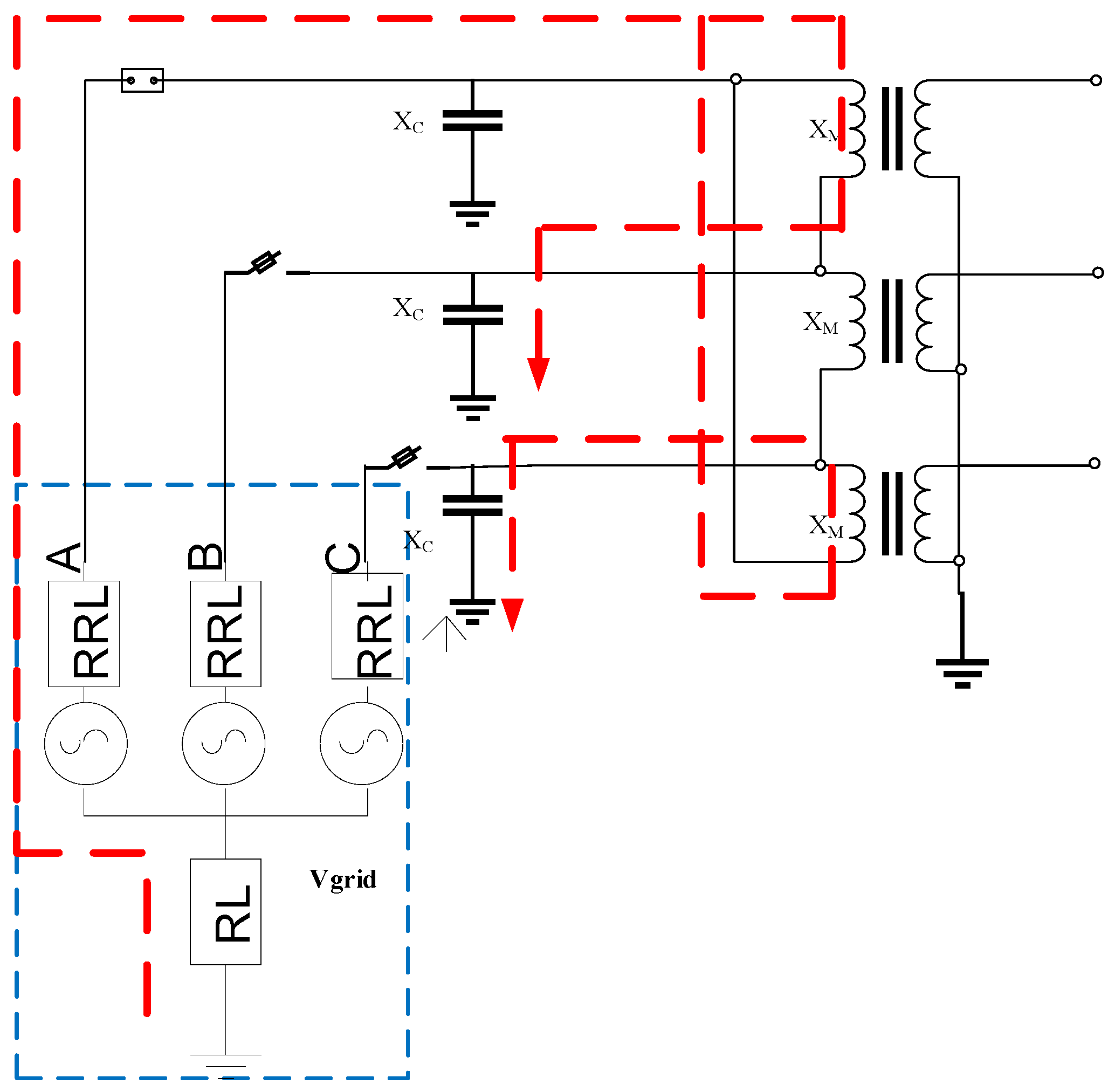
2.1. Ferroresonance in the Transformer

There are basically four different ferroresonance modes that can happen in a power system, that is, the fundamental mode, the subharmonic mode, the quasi-periodic mode and the chaotic mode, as shown in Figure 2.

• Fundamental mode

The signal has the same period as the power system ($T$). The frequency spectrums consist of the fundamental frequency component followed by the decreasing magnitude of the $n$-th odd harmonic.

• Subharmonic

The signal has a period which is a multiple of the source period ($nT$). The frequency spectrums consist of the fundamental frequency component followed by the decreasing contents of the $n$-th subharmonic.

• Quasi-periodic

The signal is not periodic but has the repetitive pattern. The frequency spectrums are discontinuous and defined as $n{f}_1+m{f}_2$, where $n$ and $m$ are integers.

• Chaotic

The signal is not periodic and the frequency spectrums are continuous.

In order to achieve the analytical solution of ferroresonance, the simplified equivalent circuit of the transformer, which consists of a nonlinear inductance, equivalent capacitance, equivalent resistance, and energy source, is considered as shown in Figure 3.

Suppose that the magnetization curve of the nonlinear inductance is represented in Figure 4, therefore, this curve can be approximated by the $n$th-order polynomial

$$i_L=a\phi +b{\phi }^n$$

(1)

where $i_L$ is a magnetizing current, $\phi$ is a magnetic flux in the transformer core, $a$ is a coefficient of the linear term that corresponds to unsaturated magnetizing inductance and $b$ is a coefficient of the nonlinear term.

The analytical solution of ferroresonance in Figure 3 can be achieved by the harmonic balance method. The differential equation for the flux linkage with the magnetization curve approximated by Equation (1) is presented by

$$\frac{d^2\phi }{d{t}^2}+\frac{1}{RC}\frac{d\phi }{dt}+\frac{1}{C}(a\phi +b{\phi }^n)={\omega }_{s}E\cos {\omega }_{s}t$$

(2)

In order to achieve the steady-state flux $\phi$ by the harmonic balance method, a simplified version of Equation (2) can be written in the form of Duffin’s equation [31,32]

$$\frac{d^2\phi }{d{t}^2}+\frac{1}{RC}\frac{d\phi }{dt}+{\omega }_0^2\phi +{\omega }_2^2{\phi }^n={\omega }_{s}E\cos {\omega }_{s}t$$

(3)

where ${\omega }_0=\sqrt{\frac{a}{C}}$ and ${\omega }_2=\sqrt{\frac{b}{C}}$.

For the fundamental mode ($n=1,3,5,\dots$), the steady-state solution of Equation (2) is written in the form

$$\phi =\mathsf{\Phi }\sin ({\omega }_{s}t+\theta )={\mathsf{\Phi }}_x\sin {\omega }_{s}t+{\mathsf{\Phi }}_y\cos {\omega }_{s}t$$

(4)

where $\mathsf{\Phi }=\sqrt{{\mathsf{\Phi }}_x^2+{\mathsf{\Phi }}_y^2}$ and $\theta ={\tan }^{-1}\left(\frac{{\mathsf{\Phi }}_y}{{\mathsf{\Phi }}_x}\right)$.

We substitute Equation (4) into Equation (2) and apply the approximation of term ${\sin }^n({\omega }_{s}t+\theta )$ with

$${\sin }^n({\omega }_{s}t+\theta )\cong k_1\sin ({\omega }_{s}t+\theta )$$

(5)

where $k_1=\frac{{(-1)}^{n-1}}{2^{n-2}}\left(\begin{array}{c}n\\ \frac{n-1}{2}\end{array}\right)$.

Then when we equate the $\sin {\omega }_{s}t$ term and neglect $\cos {\omega }_{s}t$ with the higher order terms, the following equations are obtained:

$$[-({\omega }_s^2-{\omega }_0^2)+k_1{\omega }_2^2{\mathsf{\Phi }}^{n-1}]{\mathsf{\Phi }}_x-\left(\frac{{\omega }_s}{RC}\right){\mathsf{\Phi }}_y=0$$

(6)

$$[-({\omega }_s^2-{\omega }_0^2)+k_1{\omega }_2^2{\mathsf{\Phi }}^{n-1}]{\mathsf{\Phi }}_y+\left(\frac{{\omega }_s}{RC}\right){\mathsf{\Phi }}_x={\omega }_{s}E$$

(7)

When Equations (6) and (7) are solved for the coefficients ${\mathsf{\Phi }}_x,{\mathsf{\Phi }}_y$, the solution of Equation (4) can be obtained. Finally, the solution for the other modes of ferroresonance can be achieved with similar procedures.

Ferroresonance can be explained by using a graphical approach. Consider the V-I characteristics of inductance and capacitance, as shown in Figure 5.

Since the inductive reactance of the transformer core consists of two regions, linear and nonlinear characteristics, the possible operation points are obtained as the intersection of $V_L$ and $V_S+V_C$ are as follows:

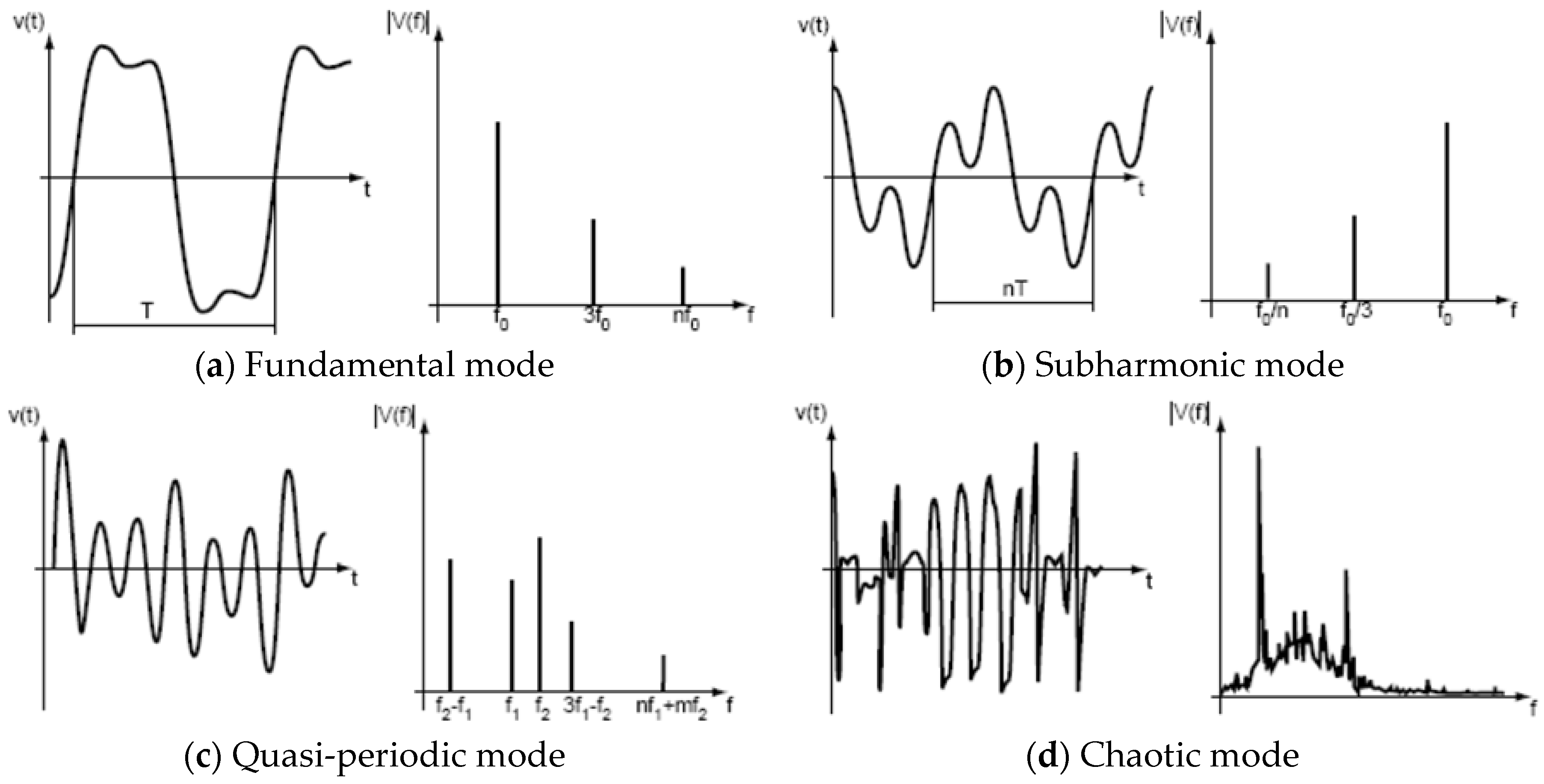
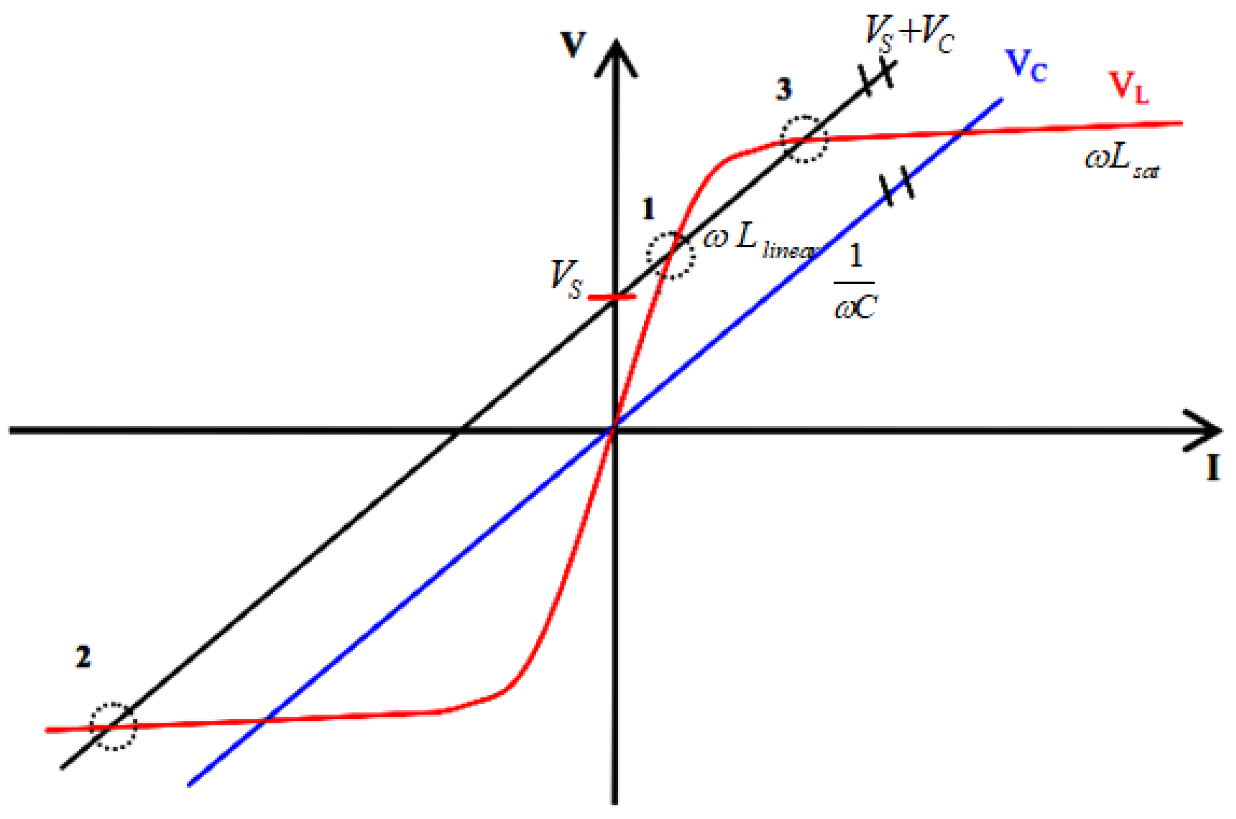
• Point 1 is a stable non-ferroresonance mode. At this point, the circuit is working with the inductive mode and remains there in the steady-state.
• Point 2 is a stable ferroresonance mode. At this point, the circuit is working with the inductive mode with both high voltage and current. This solution also remains there in the steady-state.
• Point 3 is an unstable mode and the solution will not remain there in the steady-state.

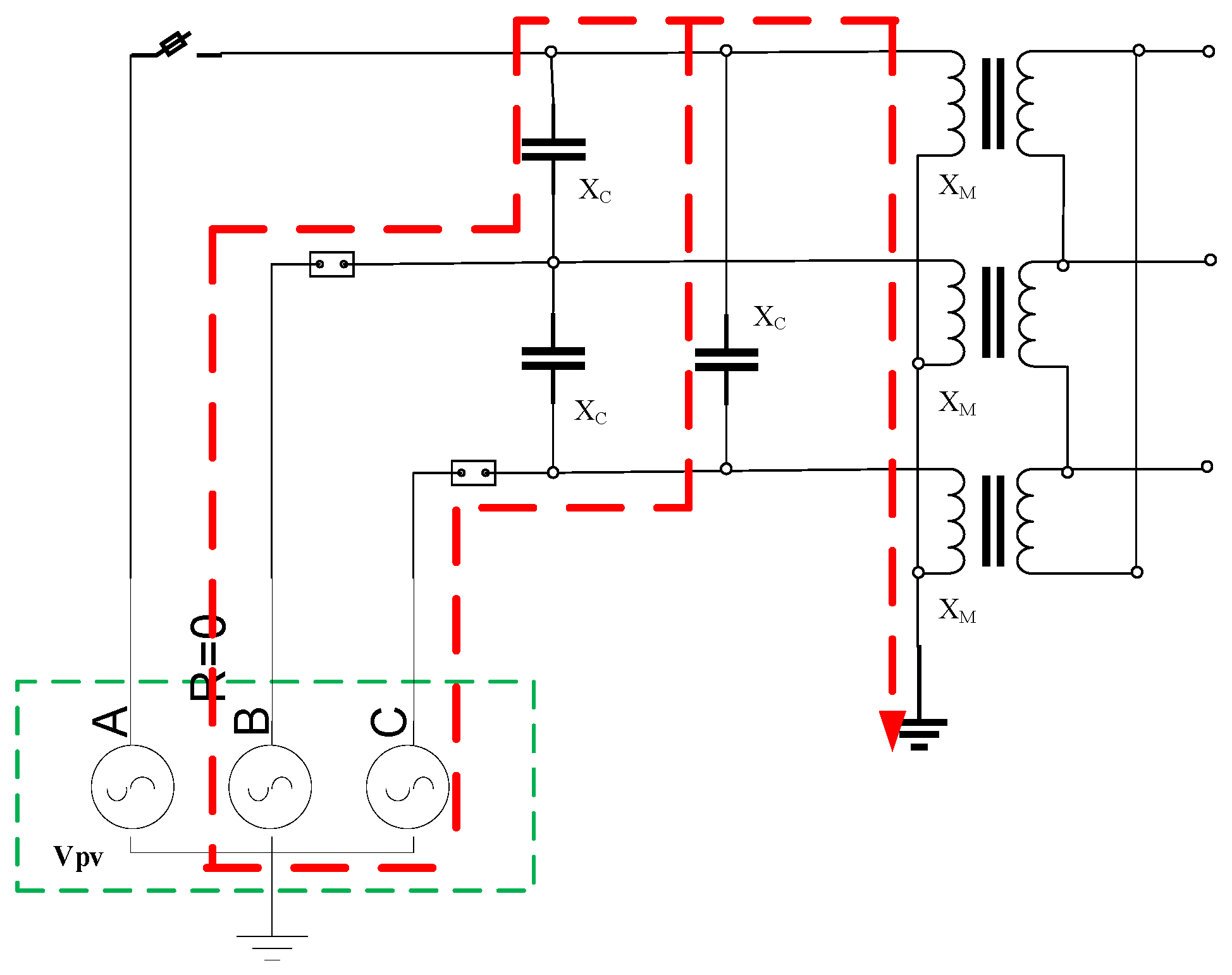
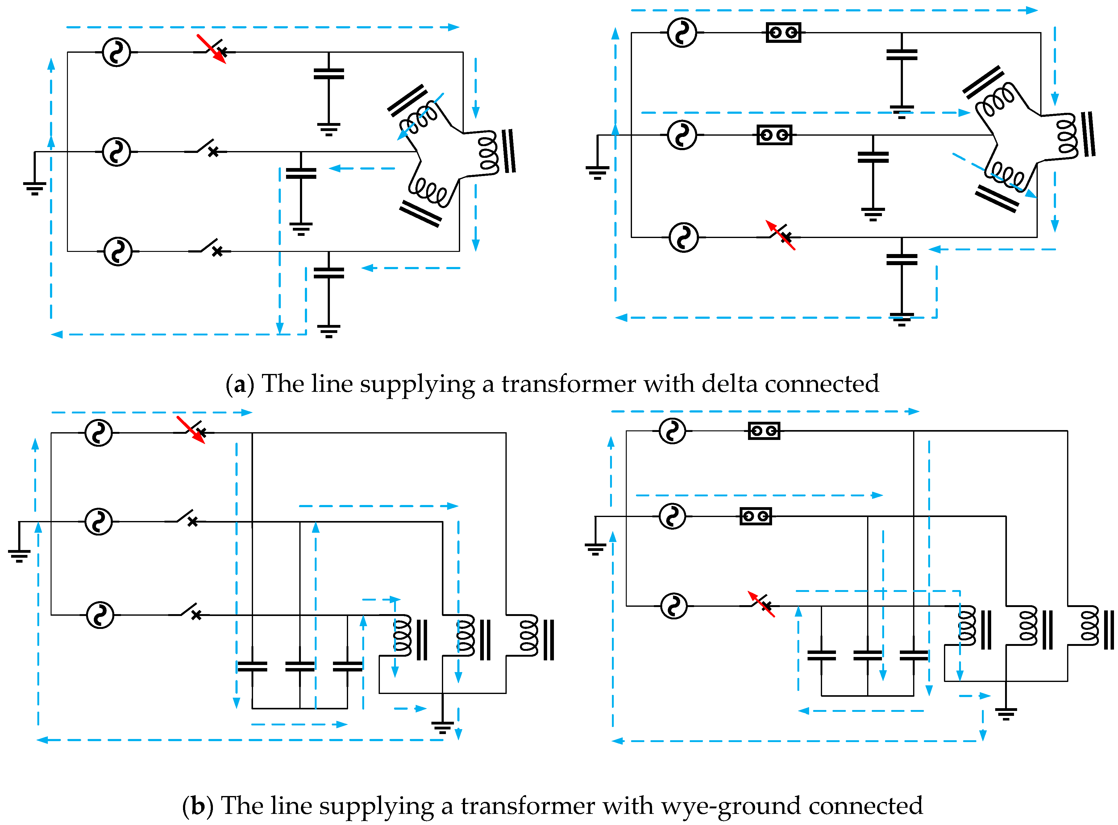
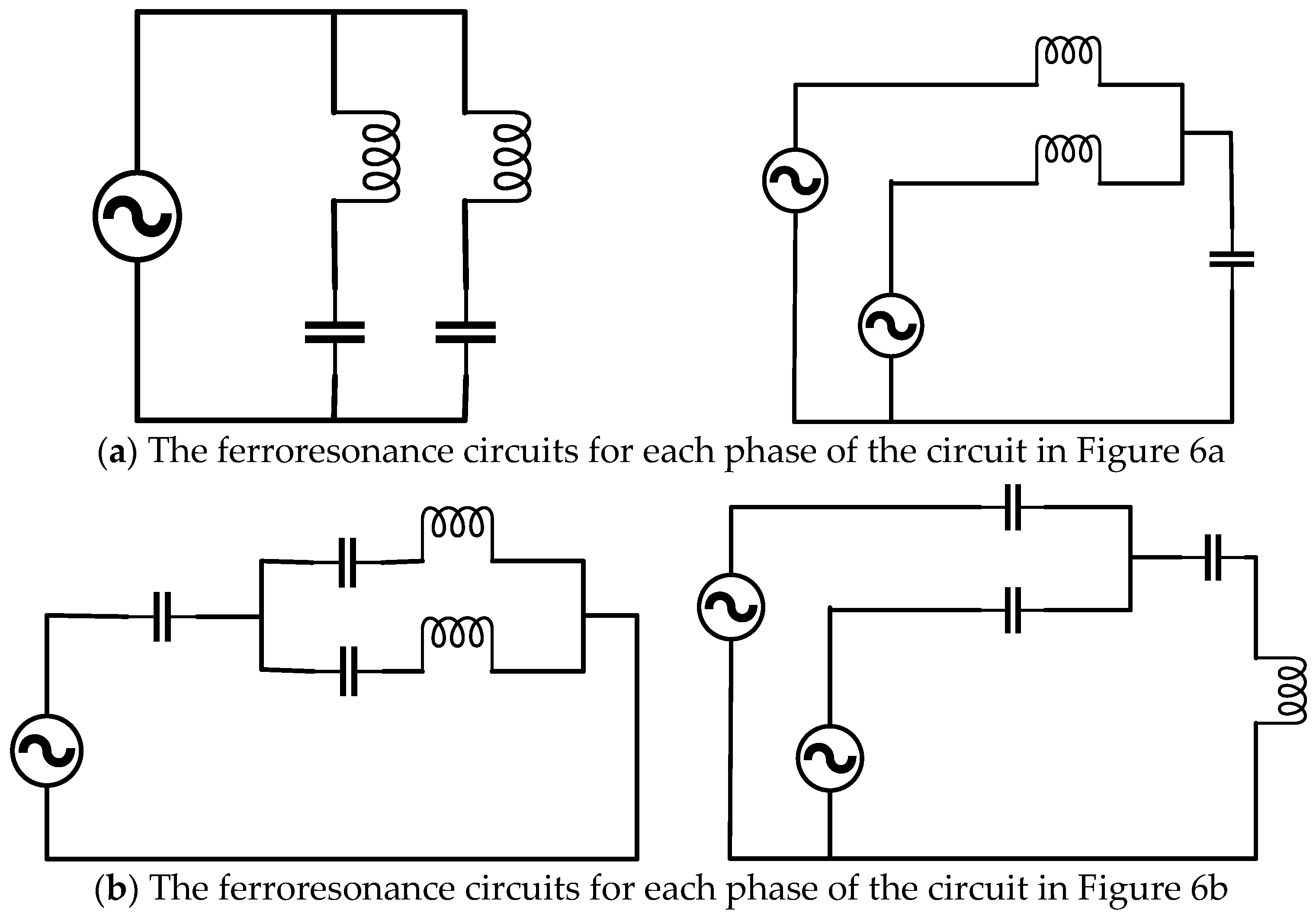
2.2. The Distribution Transformer under the Emerged or De-Energized Modes

The delta and wye transformer connection with energy sources is modeled in the form of an inductor and capacitor network as shown in Figure 6a,b, respectively. These capacitors exist in the underground cables or the overhead power lines with respect to earth. Whereas the inductors represent the magnetizing inductance of the transformers.

From the connection scheme in Figure 6, the series circuit of the capacitor, inductor and supply source is used for analyzing the ferroresonance in each phase, as shown in Figure 7.

3. System Modeling for Simulation

In this section, the modeling of the distribution system with a PV connected system is arranged. Since an experiment with ferroresonance is a destructive experiment, the demonstration is simulated using the PSCAD/EMTDC software. In this study, three different cases are considered.

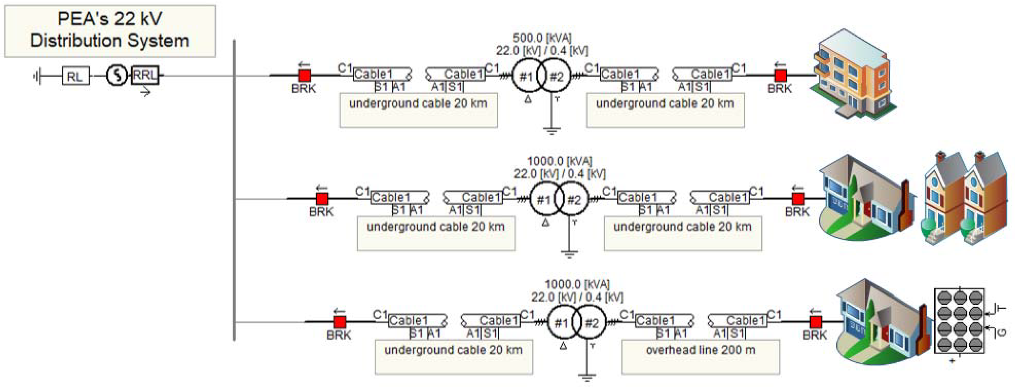
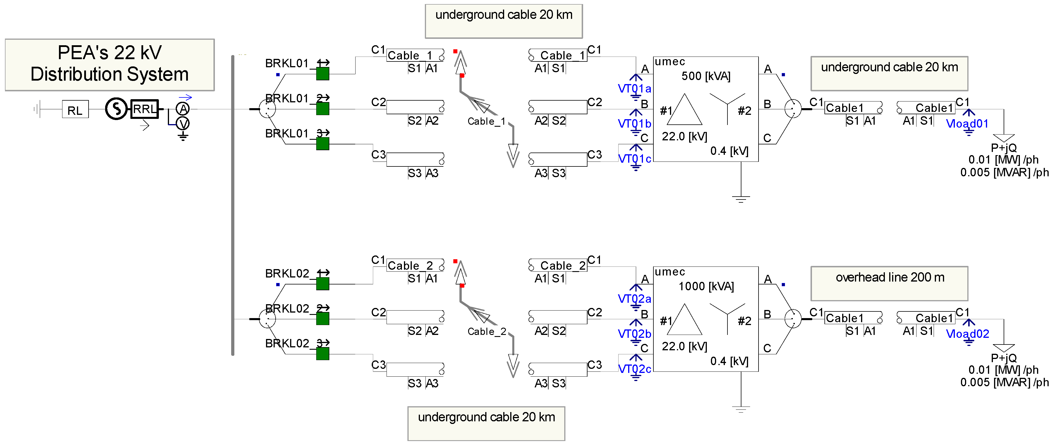
3.1. The System Under Considering

The system consists of a local load of the PEA network. Through the 22 kV distribution system, the local load has 3 transformers (one unit of 1 MVA and two units of 500 kVA) for condos, suburban homes and townhouses, and suburban homes with total installed PV rooftops, respectively. The total 500 kW installation capacity of the PV rooftop system consists of a PV array with Maximum Power Point Tracking (MPPT) and the simplified inverter without the anti-islanding system. The produced energy is incorporated into the 22 kV grid through the step-up transformer. The distribution line to the system consists of two underground cables of 20-km length and a PI transmission line section of 200-m length. Moreover, there are three cutout switches at every connection line, as shown in Figure 8.

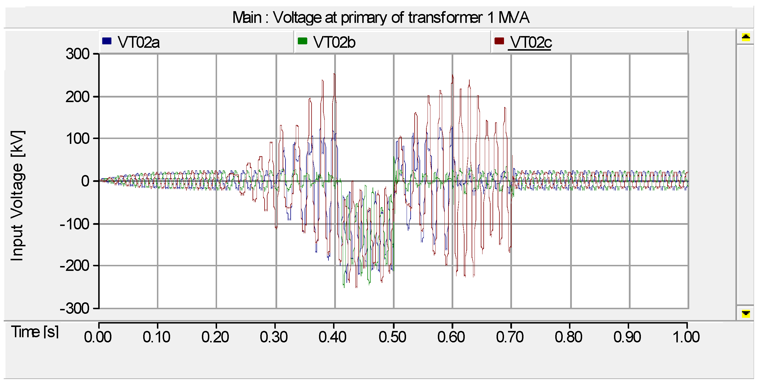
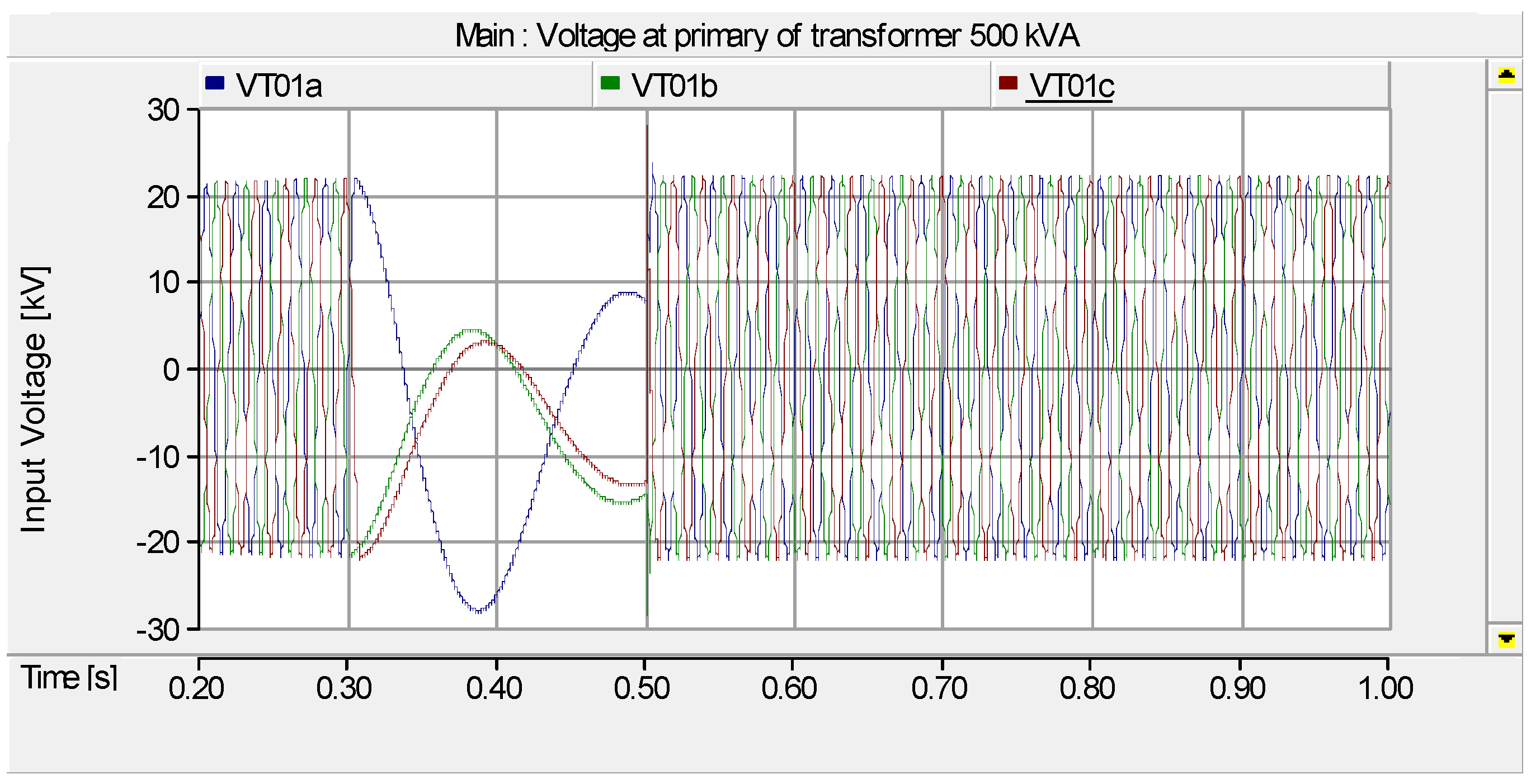
3.2. Simulation Case I: The Effect of Ferroresonance on the High Voltage (HV) Side of the Distribution Transformer

The purpose of Case I is to consider the effect that ferroresonance causes due to the connection of a 1 MVA and 500 kVA transformers to a PV system. The single line diagram of this case is shown in Figure 9 and its corresponding series inductance and capacitance (LC) ferroresonance circuit is modeled in Figure 10. Moreover, the required parameters and data are summarized in

Table 1. The parameters for simulation Case I.

Name	Parameter	Value
Vgrid	Base MVA (3 phase)	10 MVA
	Base voltage (L-L, RMS)	32 kV
	Base frequency	50 Hz
Cable 1	Steady-state frequency	50 Hz
	Segment length	20 km
Cable 2	Steady-state frequency	50 Hz
	Segment length	20 km
T1	Transformer MVA	500 kVA
	Primary voltage	22 kV
	Secondary voltage	0.4 kV
	Type: Delta-Wye ground
	Base operation frequency	50 Hz
T2	Transformer MVA	1 MVA
	Primary voltage	22 kV
	Secondary voltage	0.4 kV
	Type: Delta-Wye ground
	Base operation frequency	50 Hz
Load 1	Customer Load 1	0.01 MW + 0.005 MVAR per phase
Load 2	Customer Load 2	0.01 MW + 0.005 MVAR per phase

.

Three single-phase circuit breakers (BRK) are connected with underground cables (BRKL01_1, BRKL01_2, BRKL01_3, BRKL02_1, BRKL02_2, and BRKL02_3). The measuring equipment is represented by VT01a, VT01b, VT01c, VT02a, VT02b, and VT02c. Single-phase circuit breakers are consequently switched from phase C, A and B for de-energization. After that, they are switched from phase B, A and C for energization.

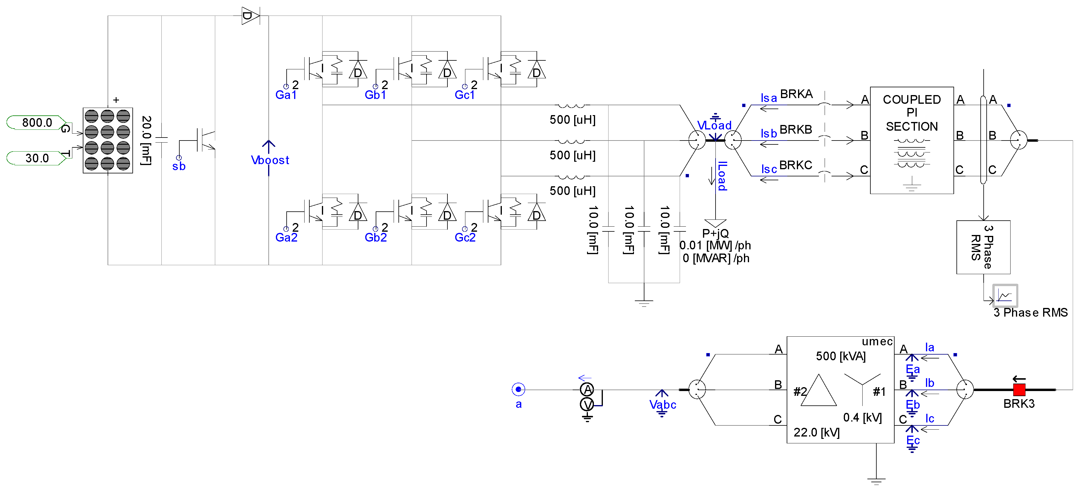
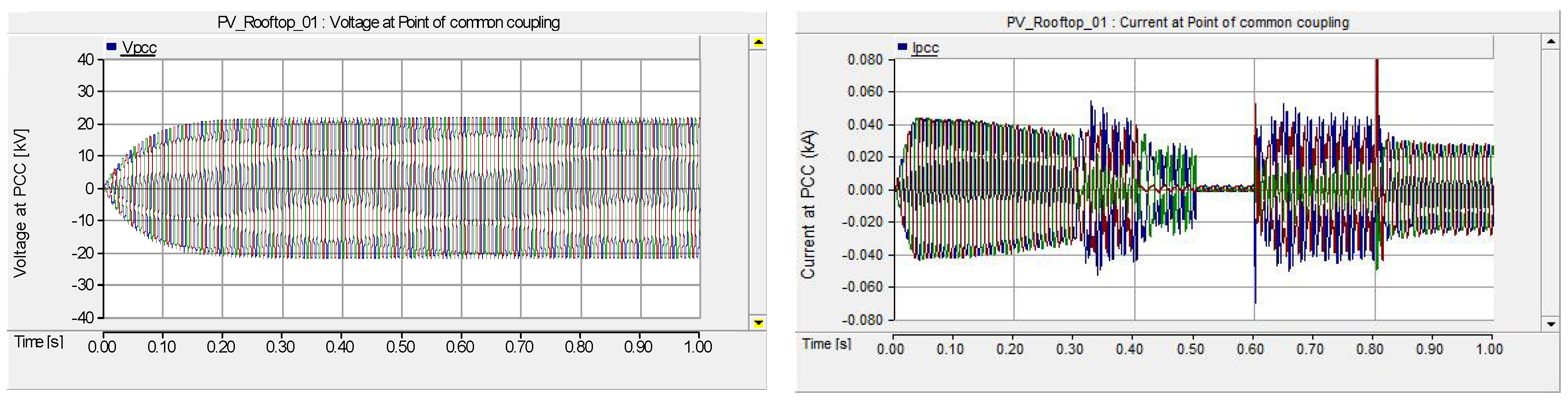
3.3. Simulation Case II and Case III: The Impact of the PV Rooftop System on the Distribution Transformer and Suburban Homes

The purpose of Case II is to consider the effect of ferroresonance that is caused by the cuts in the PV system at the interconnection transformers 500 kVA LV and suburban home sides. The purpose of Case III is to consider the effect of ferroresonance that is caused by the cuts in the PV system at the interconnection transformer 500 kVA LV side with the increasing installation capacity of the PV system step by step and to observe the effects of the change. The single line diagram for expressing these two cases is shown in Figure 11 and its corresponding series LC ferroresonance circuit is modeled in Figure 12. Additionally, the required parameters and data are summarized in

Table 2. The parameters for simulation Cases II and III.

Name	Parameter	Value
PV module data	Ref. irradiance	1000 W/m2
	Ref. Temperature	25 °C
	Effective area per cell	0.01 m2
	Series resistance per cell	0.02 $\mathsf{\Omega }$
	Shunt resistance per cell	1000 $\mathsf{\Omega }$
	Diode ideality factor	1.5
	Band gap energy	1.103 eV
	Saturation current at reference conditions per cell	1 × 10−12 kA
	Short circuit current at the ref. conditions per cell	0.0025 kA
	Temperature Coefficient of photocurrent	0.001 A/K
Coupled PI Section	Line Rated Frequency	50 Hz
	Line Length	0.2 km
T3	Transformer MVA	500 kVA
	Primary voltage	0.4 kV
	Secondary voltage	22 kV
	Type: Wye ground—Delta
	Base operation frequency	50 Hz
Load 3	Customer Load 3	0.01 MW per phase

.

Three single-phase circuit breakers are connected with the transmission line PI section (BRKA, BRKB, and BRKC). The measuring equipment is represented by Ea, Eb, Ec, Ia, Ib, Ic, VLoad and ILoad. Single-phase circuit breakers are consequently switched from phase B, C and A for de-energization. After that, they are switched from phase A, C and B for energization.

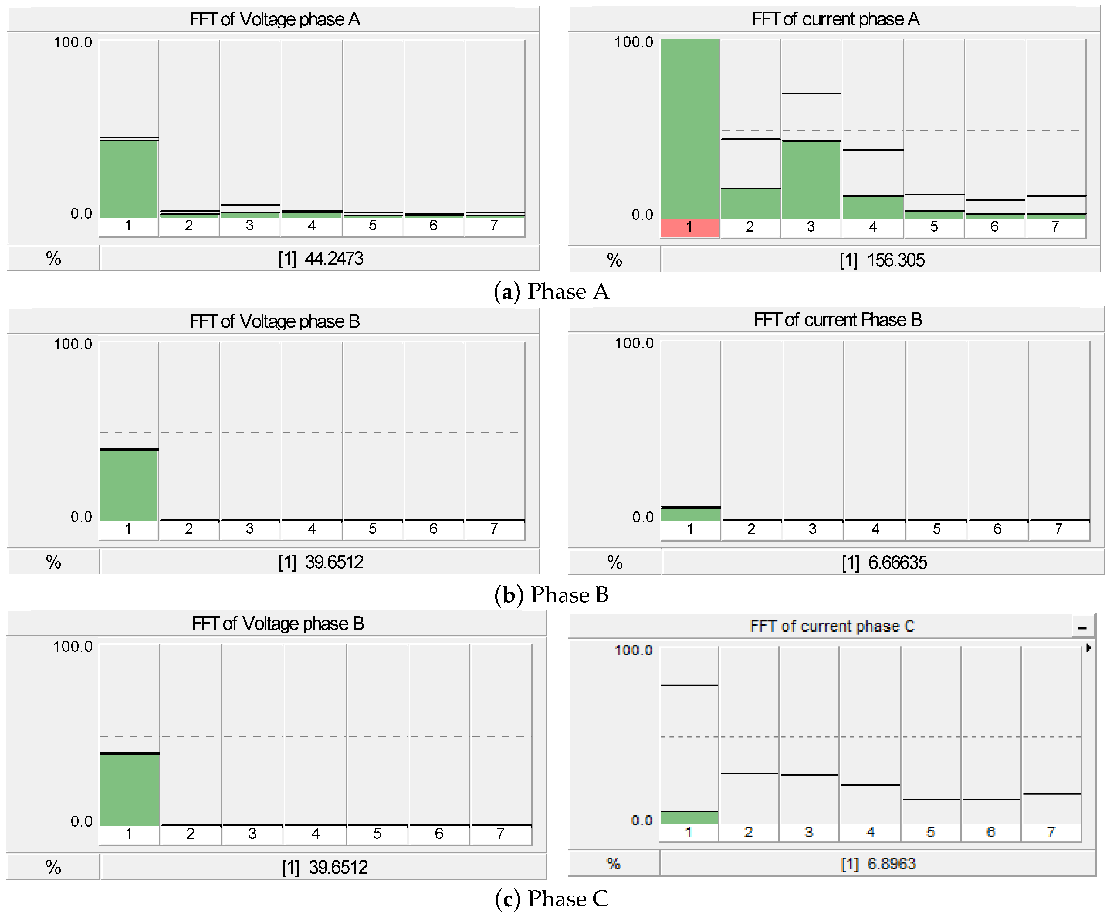
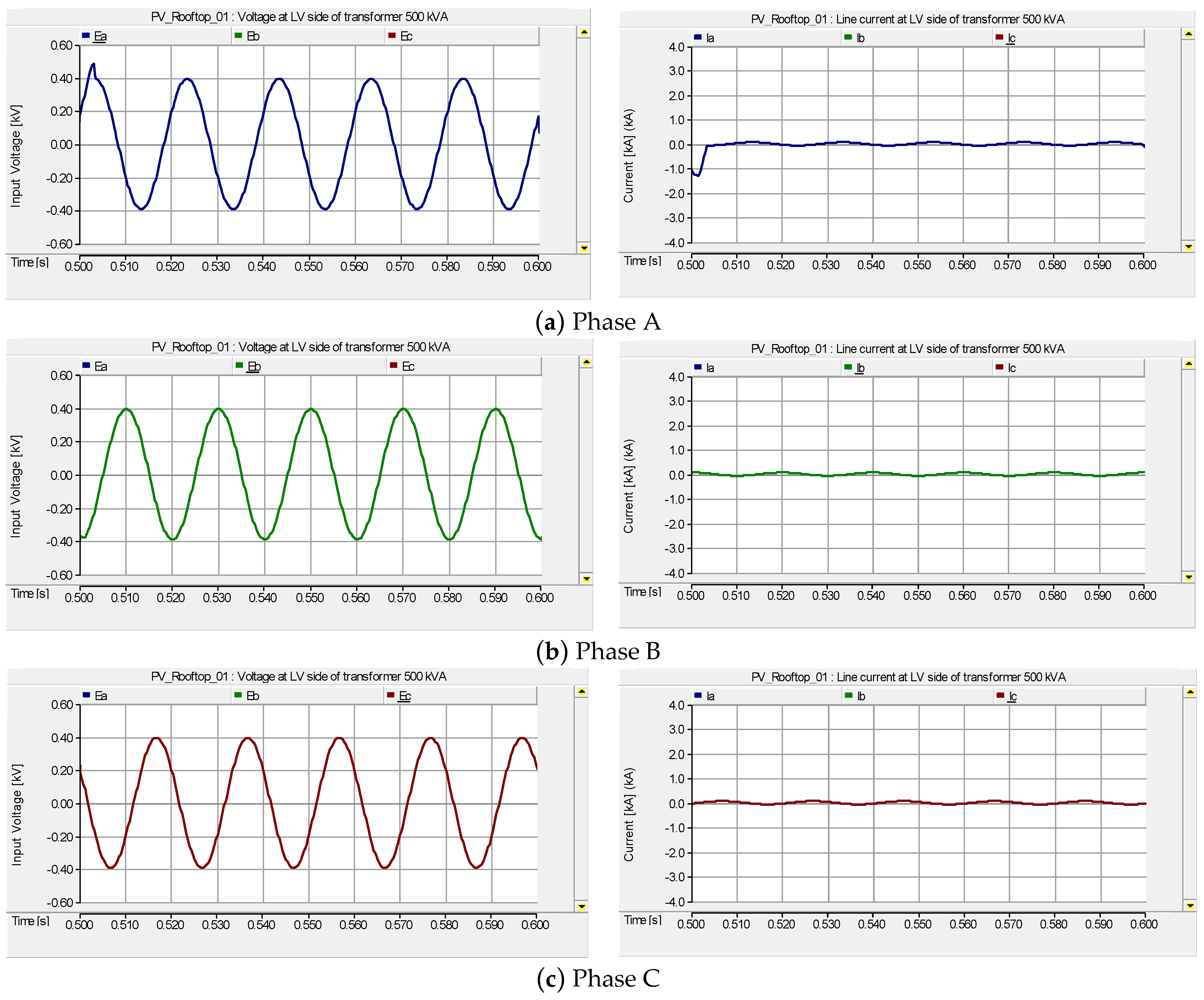
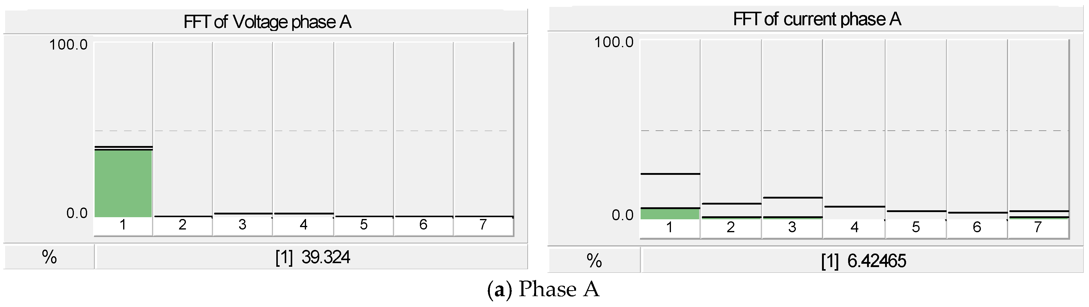
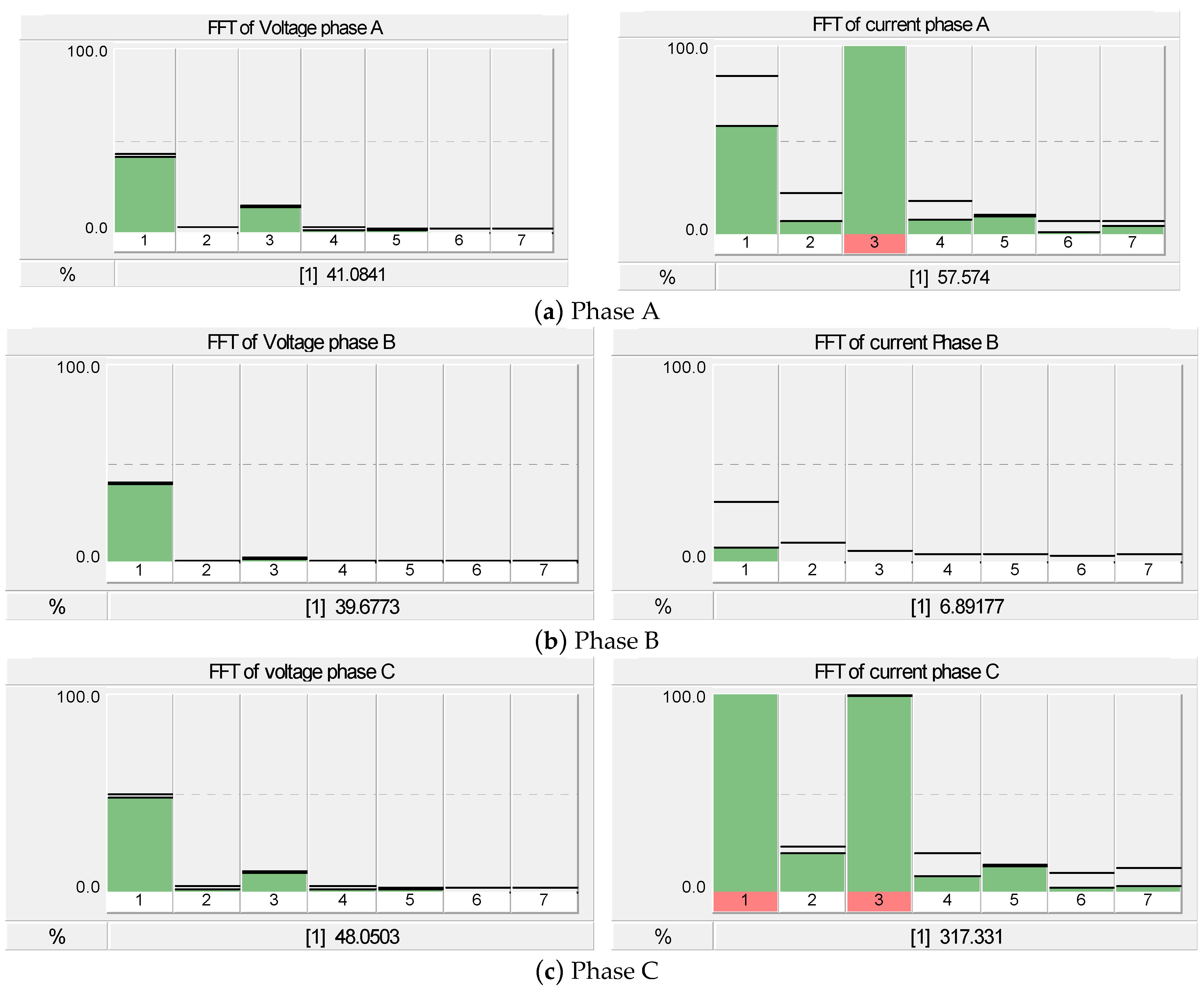
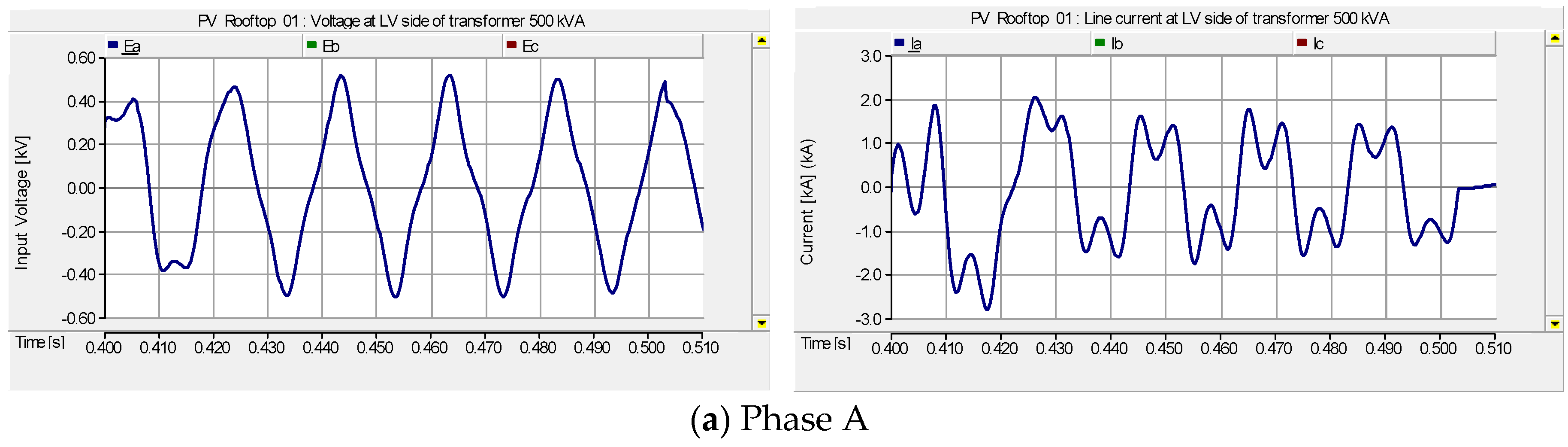
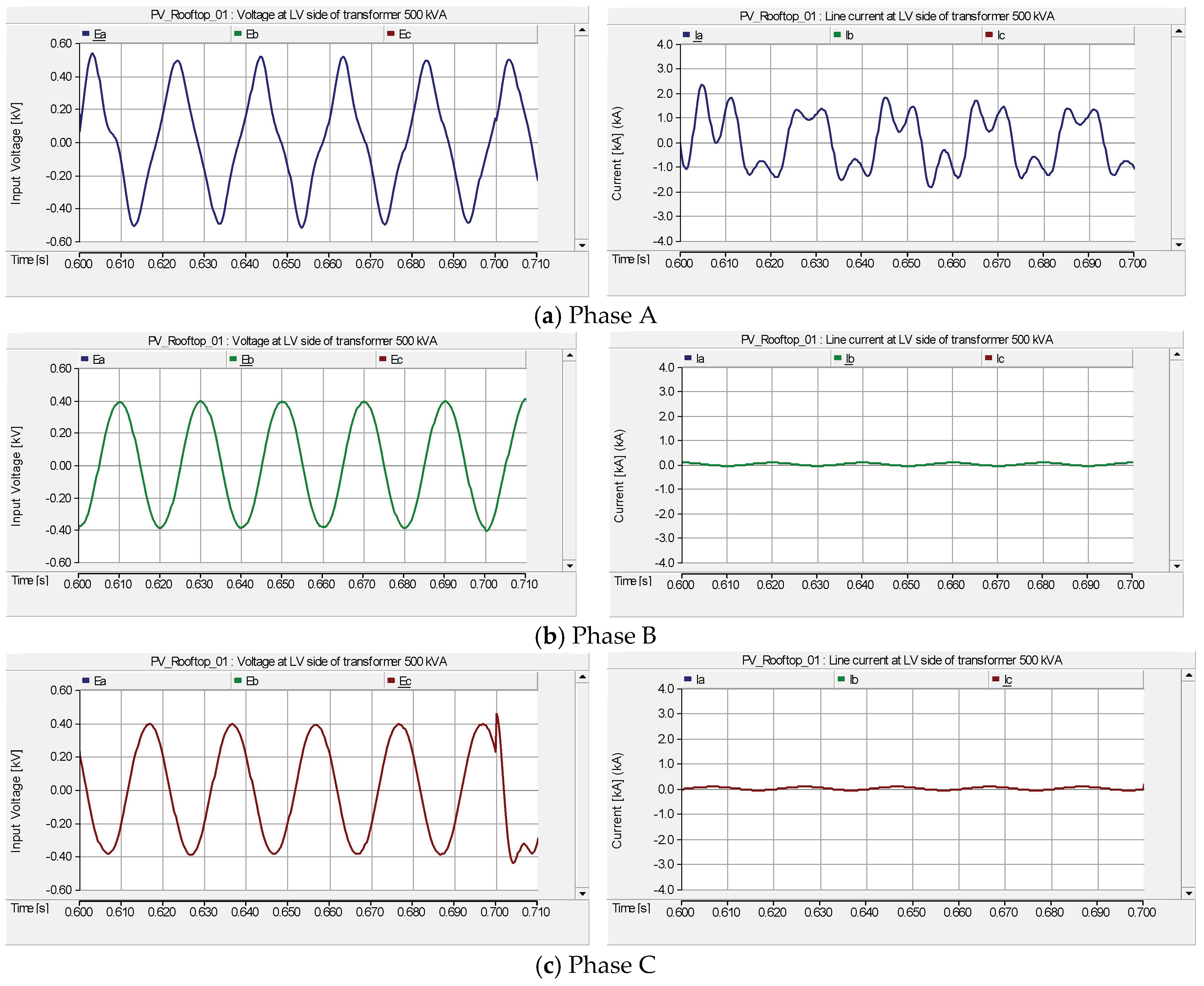
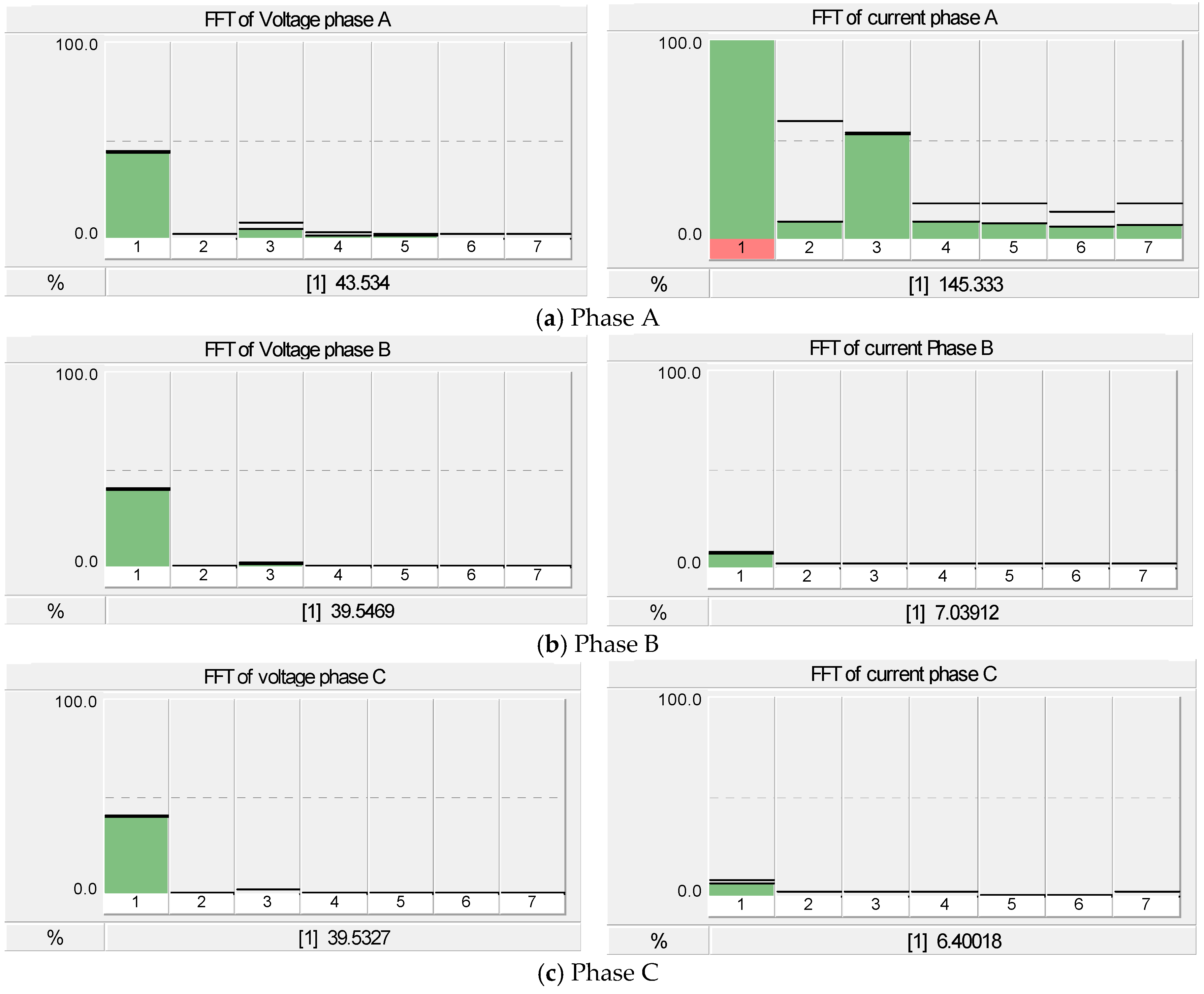
4. Simulation Results and Discussion

The simulation results from the model in Section 3 are considered, analyzed and discussed in this section.

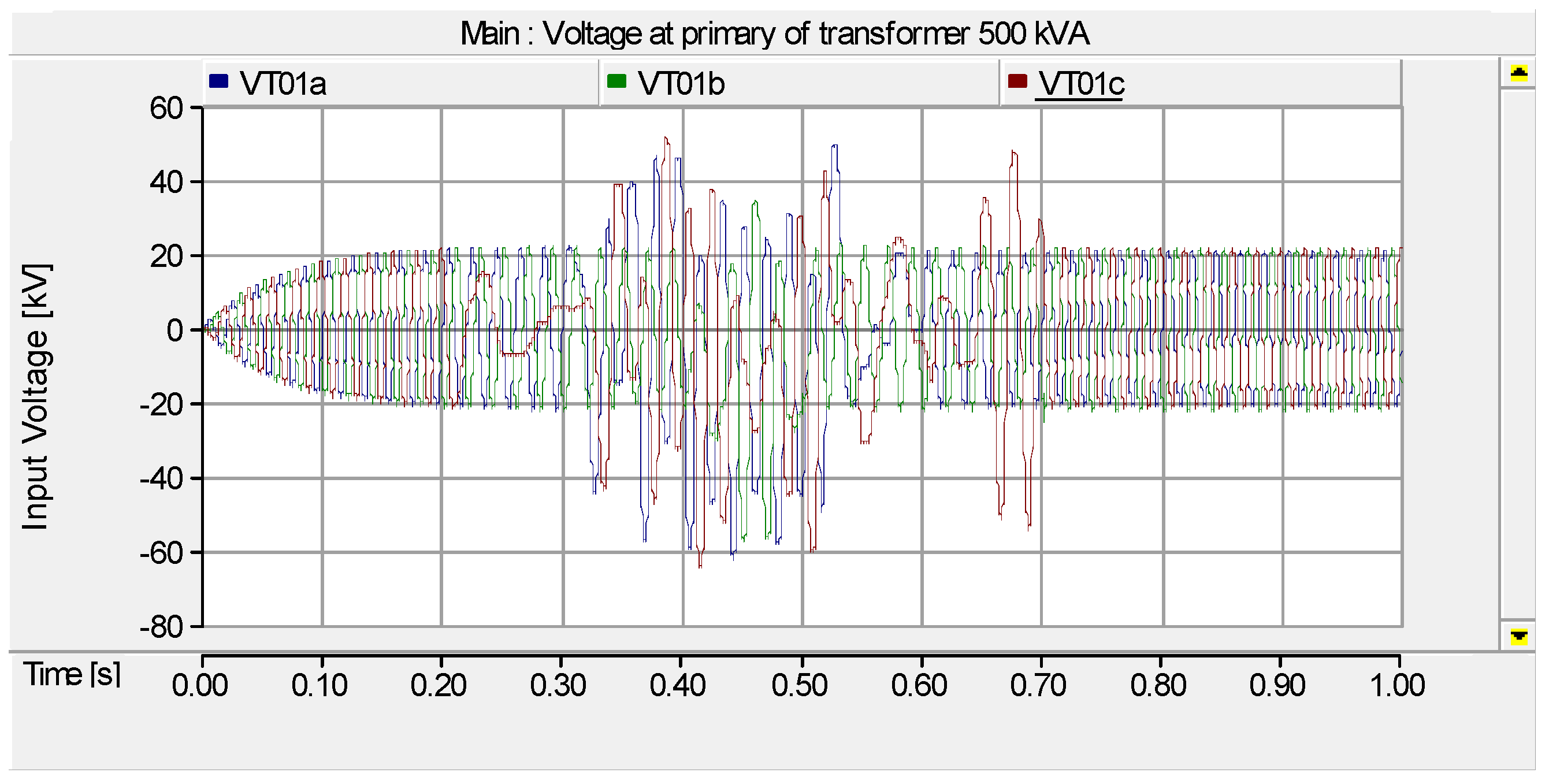
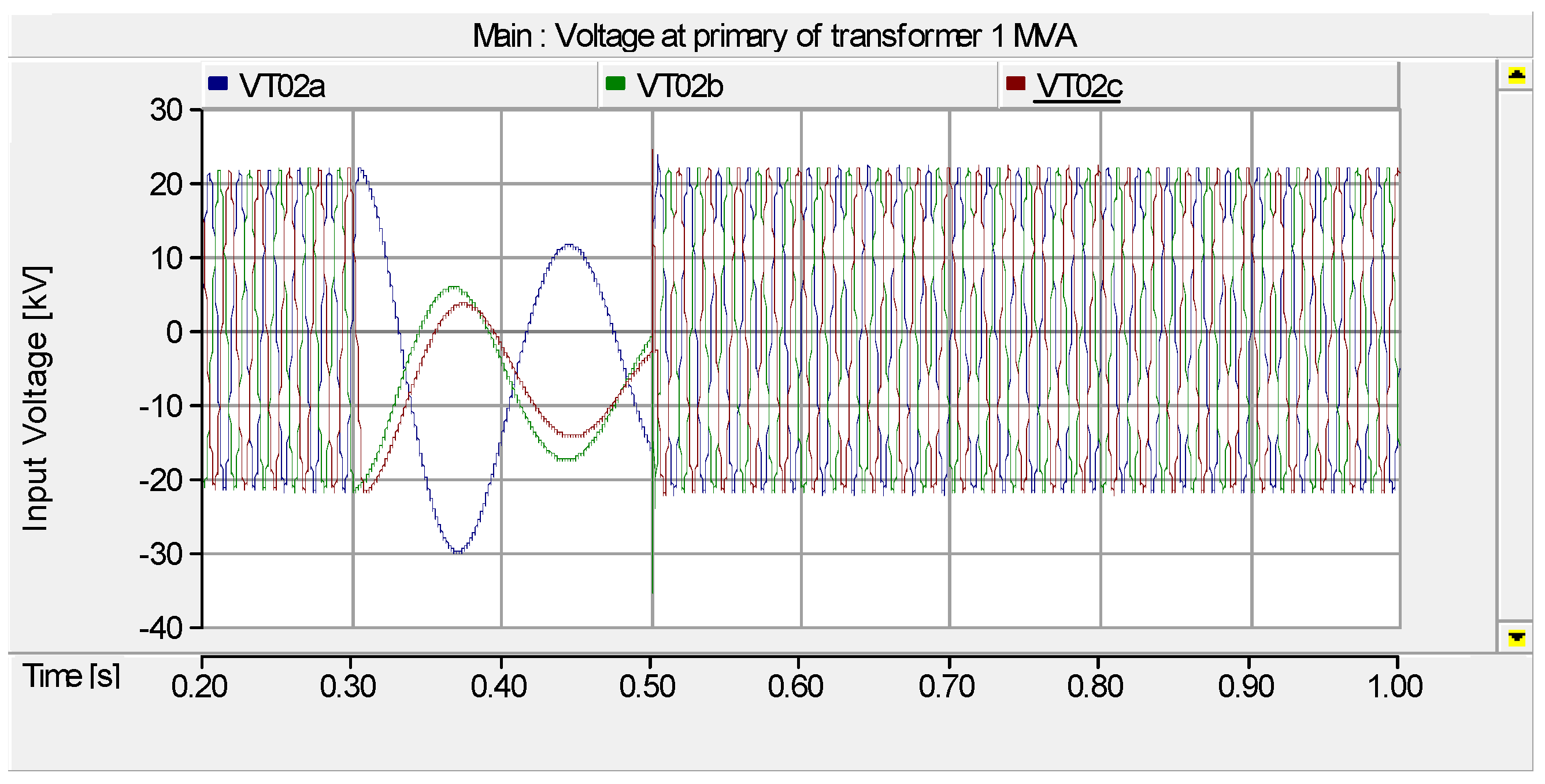
4.1. Case I: The Ferroresonance Effect on the 500 kVA and 1 MVA Transformer with Condos, Suburban and Town House Loads

For Case I, the single-phase de-energization and energization at BRKL01 and BRKL02 illustrate the ferroresonance overvoltage of the 1 MVA and 500 kVA transformers. The simulation results also show that the overvoltage occurs between 0.25–0.7 s as seen in Figure 13 and Figure 14, respectively.

However, ferroresonance does not occur when the distribution transformer is not in the saturation region and the three-phase circuit breaker is connected and disconnected at the same time. These characteristics are shown in Figure 15 and Figure 16, respectively.

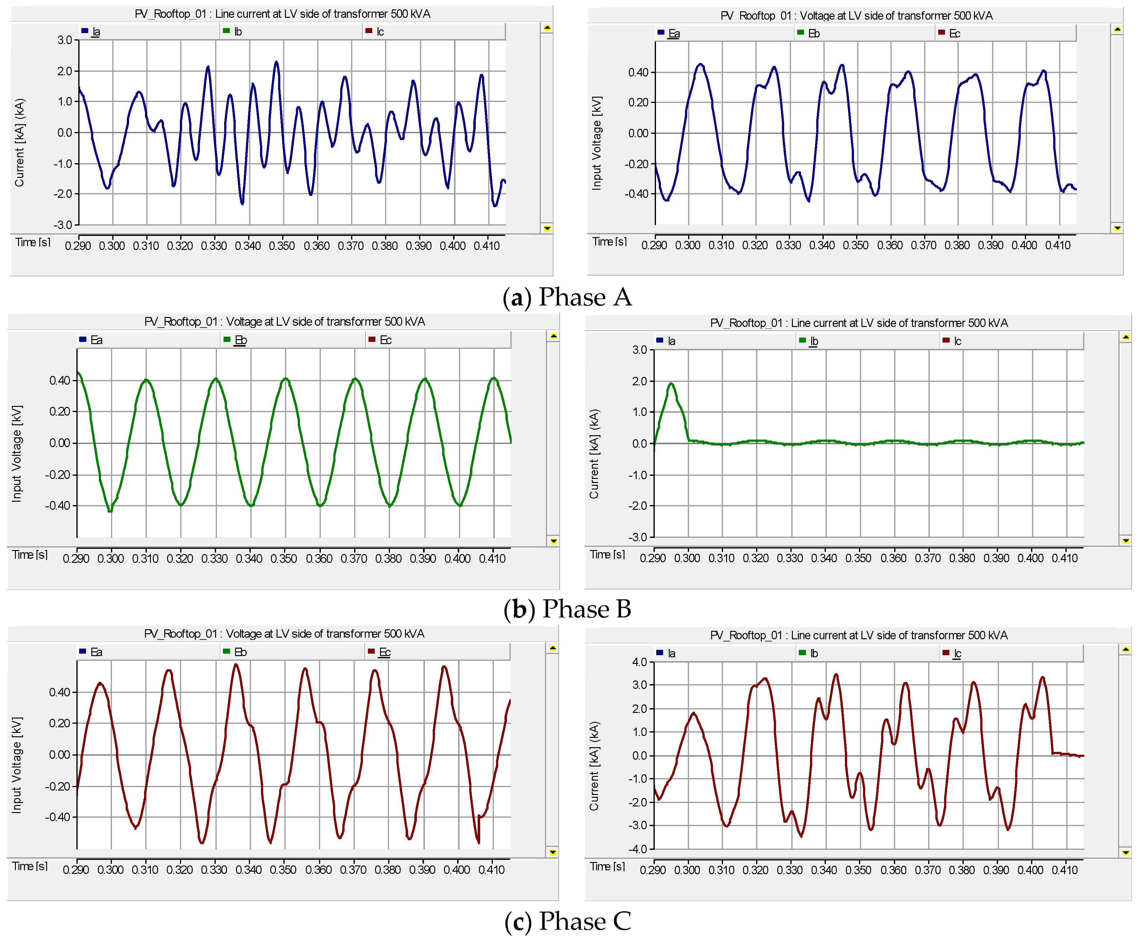
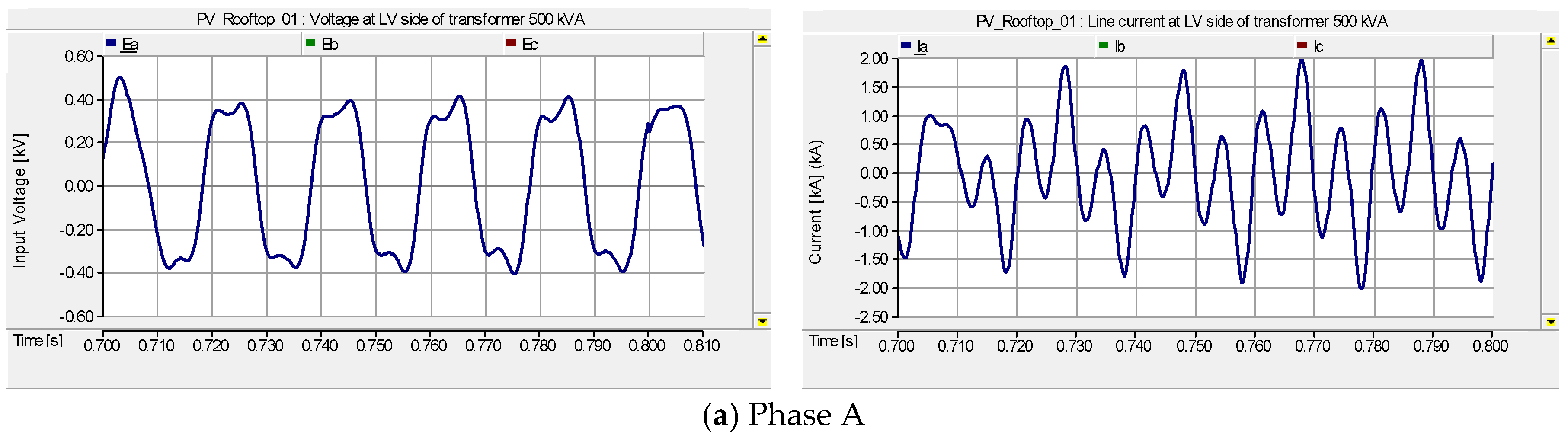
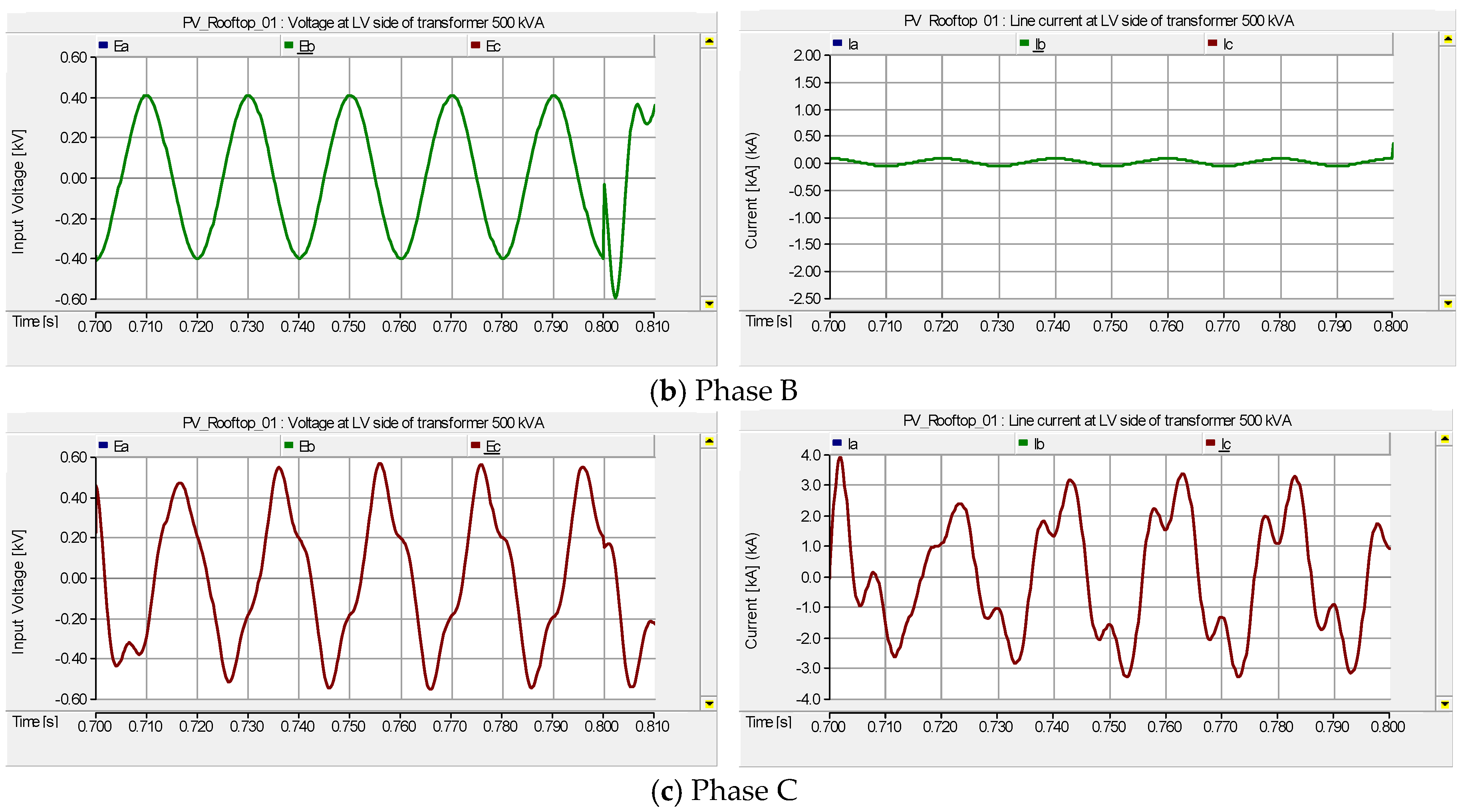
4.2. Case II: The Ferroresonance Effect on the 500 kVA Transformer LV Side with Suburban Home Load and the Total 500 kW Installation Capacity of PV Rooftop Systems

In Case II, the de-energization and energization in the phase by phase scheme are illustrated. First, the BRKB opens at 0.3 s. The corresponding phase voltage and current are shown in Figure 17.

The frequency analysis results is shown in Figure 17. The corresponding frequency spectrums are obtained as shown in Figure 18.

From the results in Figure 17 and Figure 18, it is clearly seen that phase A and C are affected by the ferroresonance. Their voltage consists of the fundamental mode ferroresonance while the current consists of the combination of fundamental mode and quasi-periodic mode ferroresonances.

Secondly, a phase C is consequently disconnected by opening BRKC at time 0.4 s. The corresponding phase voltage and current are shown in Figure 19.

The frequency analysis of the results is shown in Figure 19. The corresponding frequency spectrums are obtained as shown in Figure 20.

From the results in Figure 19 and Figure 20, it can be clearly seen that only phase A is affected by ferroresonance. Its voltage consists of fundamental mode ferroresonance while the current consists of the combination of fundamental mode and quasi-periodic mode ferroresonances.

Finally, phase A is disconnected by opening BRKA at time 0.5 s. The corresponding phase voltage and current are shown in Figure 21.

The corresponding frequency spectrums of Figure 21 are obtained and shown in Figure 22.

From the results in Figure 21 and Figure 22, the voltage and current of all phases are not affected by ferroresonance.

After all the circuit breakers are disconnected, the connection characteristics of each phase are considered. First, the BRKA is closed at 0.6 s. The corresponding phase voltage and current are shown in Figure 23.

The corresponding frequency spectrums of Figure 23 are obtained and shown in Figure 24.

From the results in Figure 23 and Figure 24, only phase A is affected by the ferroresonance. Its voltage consists of the fundamental mode ferroresonance while the current consists of the combination of the fundamental mode and quasi-periodic mode ferroresonances.

Second, the BRKC is closed at 0.7 s. This connection yields the voltage and current as shown in Figure 25.

The corresponding frequency spectrums of Figure 25 using FFT are shown in Figure 26.

From the results in Figure 25 and Figure 26, phase A and phase C are affected by ferroresonance. Their voltage consists of the fundamental mode ferroresonance while their current consists of a combination of the fundamental mode and quasi-periodic mode ferroresonances.

Finally, the BRKB is closed at 0.8 s. This connection yields the voltage and current as shown in Figure 27.

The corresponding frequency spectrums of Figure 27 using FFT are shown in Figure 28.

From the results in Figure 27 and Figure 28, phases A, B and C are affected by the ferroresonance. Their voltage consists of the fundamental mode ferroresonance while their current consists of a combination of the fundamental mode and quasi-periodic mode ferroresonances. However, the effect of this phenomenon exists for a short time.

Furthermore, the ferroresonance that occurs in the system leads the voltage and current at the suburban home to have fluctuations as shown in Figure 29.

For the HV side of the distribution transformer, its voltages are not affected by ferroresonance since it is connected to the grid. However, the currents fluctuate due to this phenomenon, as shown in Figure 30.

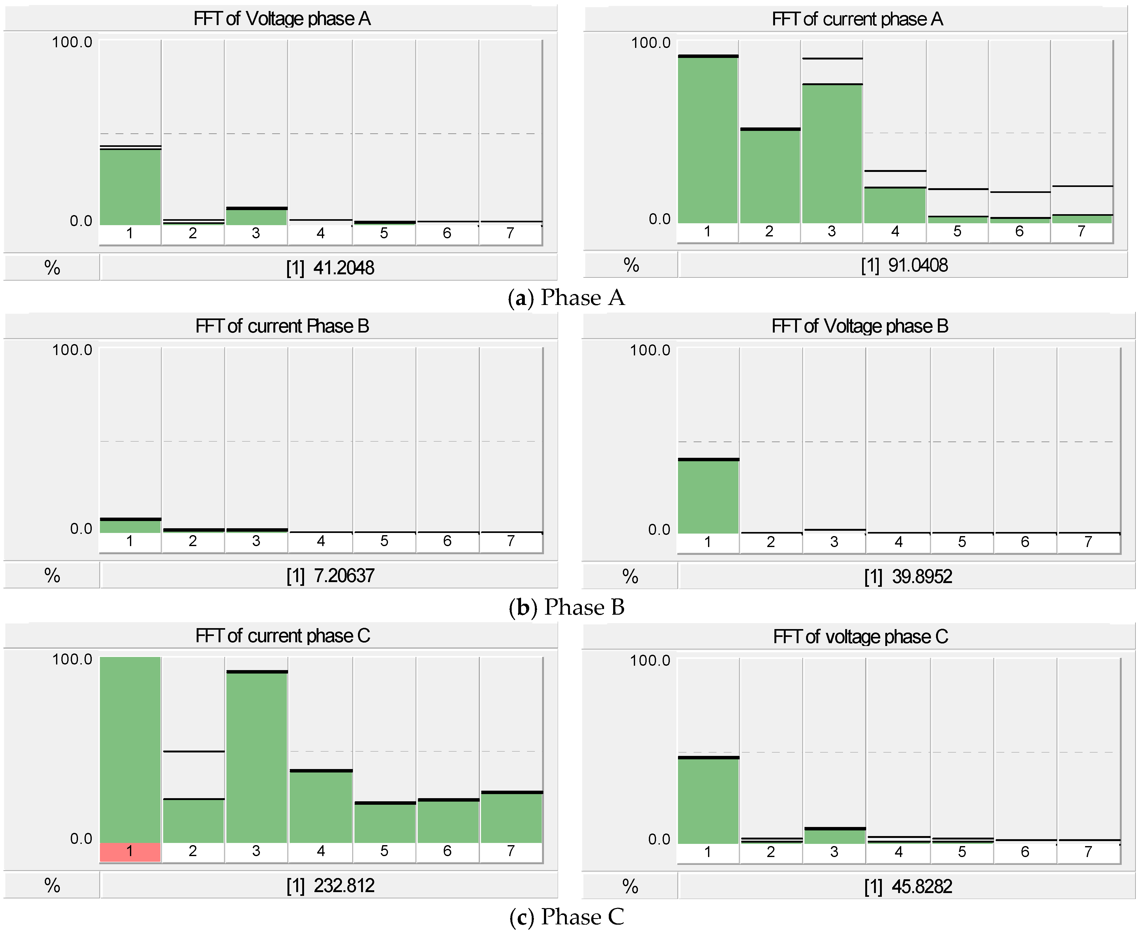
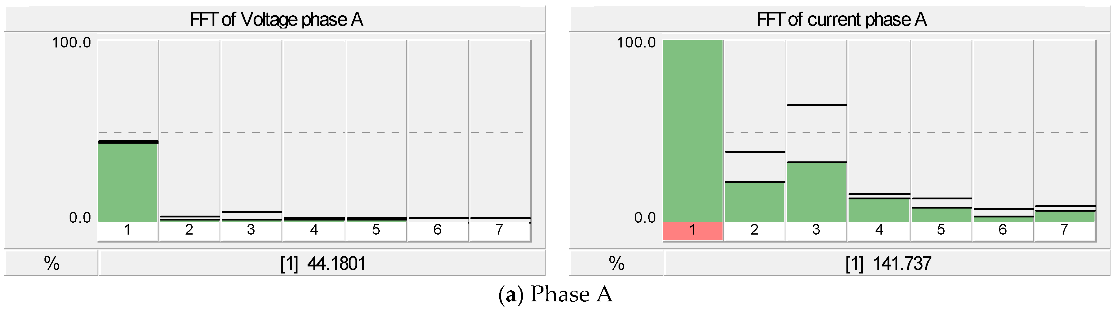
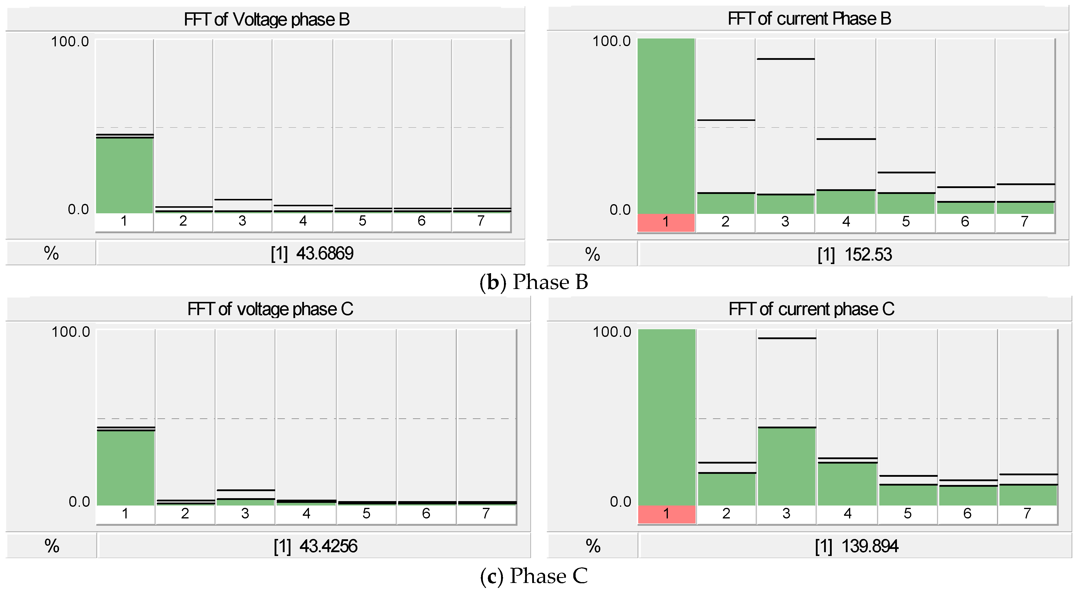
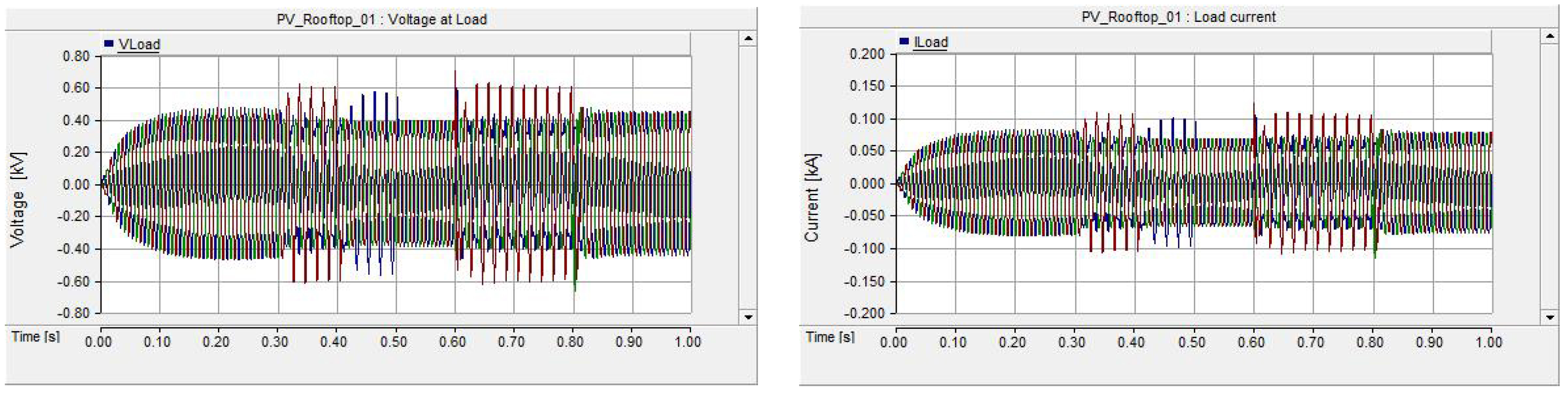
4.3. Case III: The Effect of Ferroresonance When Increasing the Capacity of PV Rooftop Systems from 1 kW to 500 kW

In Case III, the effects of the PV system connection at the 500 kVA transformer LV side with the step by step increasing of the installed capacity of the PV system are shown in

Table 3. The simulation results of the increasing installation capacity of the PV system.

PV Install Capacity (kW)	Vmax (kV, L-L) at Terminal Point of Transformer	Imax (kA) at Terminal Point of Transformer	Vload Max. (kV, L-L)	Iload Max. (kA)	Max. HD of Voltage (%)	Ferroresonance Phenomena
1	0.578	3.476	0.566	0.098	27.8	Y
2	0.578	3.665	0.576	0.100	31.4	Y
3	0.580	3.739	0.577	0.100	33.2	Y
4	0.580	3.741	0.577	0.100	33.2	Y
5	0.580	3.742	0.581	0.100	33.2	Y
6	0.580	3.743	0.577	0.100	34.1	Y
7	0.580	3.746	0.577	0.100	33.1	Y
8	0.580	3.748	0.577	0.100	33.1	Y
9	0.580	3.753	0.577	0.100	33.1	Y
10	0.580	3.758	0.577	0.100	33.1	Y
20	0.603	3.986	0.601	0.104	32.8	Y
30	0.612	4.103	0.609	0.106	32.5	Y
40	0.619	4.132	0.617	0.107	33.3	Y
50	0.639	4.274	0.638	0.111	33.2	Y
60	0.659	4.366	0.658	0.114	32.6	Y
70	0.660	4.374	0.658	0.114	31.8	Y
80	0.660	4.383	0.658	0.114	33.9	Y
90	0.668	4.524	0.668	0.116	34.2	Y
100	0.690	4.728	0.688	0.119	34.7	Y
200	0.640	4.279	0.639	0.111	31.7	Y
300	0.677	4.507	0.674	0.117	35.1	Y
400	0.698	4.647	0.696	0.121	36.3	Y
500	0.716	5.302	0.715	0.124	37.8	Y

.

Because the installation of the PV systems grid connected in Thailand is preferred from a minimum of 1 kW, Table 3 shows that a 1 kW PV system can lead to ferroresonance phenomena in the distribution transformer. In addition, the voltage and current values at the terminal transformer LV side are high. If the installed capacity of the PV system increases, the current in this area also increases and directly affects the distribution transformer.

From these results, the researcher found that the simulation results are different in some cases. The reasons for the differences are summarized as follows:

(1)

The effect of the underground cable and distribution transformer configuration.

(2)

The effect of magnetizing the core saturation from the distribution transformer used for the voltage divider.

(3)

The effect of the supply voltage to a transformer primary winding that is connected to a ground or neutral separated wye or delta connection.

(4)

The effect of the increase of the voltage source in the system which, in this case, is the PV rooftop system on the LV side.

The results reveal that the ferroresonance overvoltage and overcurrent phenomena can happen in this system under the saturation transformer with the capacitance of the 20 km underground cable, the capacitance of the 200 m transmission line PI section, the nonlinear characteristic of the 1 MVA and 500 kVA transformer, and the PV system source. Moreover, the major principle of the ferroresonance phenomena is an unbalanced switching operation. If there are differences in switching cutouts disconnected and connected, they will cause damage to the power system. The ferroresonance overvoltage will be 30–150 kV in the MV side, and the overvoltage will be 0.5–1 kV; the overcurrent will be 2–6 kA in the LV side. The effect of this situation is the generation of the destruction of the electrical equipment and protection system. For this reason, the phenomena will not happen when three-phase disconnected switching cutouts are operated at the same time. However, when three-phase switching cutouts are operated at the same time, resonance transience will happen and can produce harmonic distortion of the current in the distribution network as demonstrated in Figure 23, Figure 24 and Figure 25.

To prevent ferroresonance occurring in a transformer accidentally energized in only one or two phases (see Figure 3), the practical solutions consist of the following:

• Lowering the value of the capacitance between the circuit breaker and transformer below its critical value by using, for example, a circuit breaker cubicle closer to the transformer or placing circuit breakers just upstream of the transformers and closing them only when the voltage has been restored to all three-phases.
• Avoiding use of the transformers delivering an active power which is lower by 10% than its rated apparent power.
• Avoiding no-load energizing.
• Prohibiting single-phase operations or fuse protection, blowing of which results in single-pole breaking.
• Prohibiting live work on a cable-transformer assembly when the cable length exceeds a certain critical length.
• Resistance-earthing of the neutral of the supply substation.
• Solidly earthing the neutral (permanently or only during energizing and de-energizing operations) of a transformer whose primary is wye-connected (available neutral).

5. Conclusions

This paper presents the analysis of ferroresonance phenomena in 0.4/22 kV distribution transformers with a PV system source using the software simulation approach. The results explain that ferroresonance overvoltage and overcurrent will occur when the system consists of a PV rooftop source, the capacitance in a long transmission line, a nonlinear distribution transformer with saturation characteristic and the usage of single-phase switching cutouts in the system. In addition, when the installed capacity of the PV system increases, the current at the terminal distribution transformer also increases and causes damage to the distribution transformer. Typically, for the three-phases switching cut-out and cut-in, ferroresonance will not occur. To prevent ferroresonance in a PV grid connected system, many solutions can be applied. The usage of the three-phase switching cutouts for connecting and disconnecting the system or the multi-pole breaking switchgear is one of the solutions. Installing the ferroresonance suppression circuit to the transformer also prevents the derogation. If the single-phase switching cutouts is installed, the proper sequent switching must be considered. In addition, the distribution transformer must be in the normal condition (without saturation characteristic). Moreover, a wide overview of this phenomenon that resulted from simulation studies can help the operator in electrical maintenance departments to get quick possible solutions to the problem. Therefore, it will allow the analysis of the risks and the evaluation of the solution to be completed efficiency.

References

- Wareing, J.B.; Perrot, F. Ferroresonance Overvoltages in Distribution Networks. In Proceedings of the IEE Colloquium on Warning! Ferroresonance Can Damage Your Plant (Digest No: 1997/349), Glasgow, UK, 12 November 1997; pp. 5/1–5/7. [Google Scholar]
- Walling, R.A. Ferroresonance in Low-Loss Distribution Transformers. In Proceedings of the 2003 IEEE Power Engineering Society General Meeting, Toronto, ON, Canada, 13–17 July 2003; Volume 2, p. 1222. [Google Scholar]
- Dugan, R.C. Examples of ferroresonance in distribution. In Proceedings of the 2003 IEEE Power Engineering Society General Meeting, Toronto, ON, Canada, 13–17 July 2003; Volume 2, p. 1215. [Google Scholar]
- Dolan, E.J.; Gillies, D.A.; Kimbark, E.W. Ferroresonance in a transformer switched with an EVH line. IEEE Trans. Power Appar. Syst. 1972, PAS-91, 1273–1280. [Google Scholar] [CrossRef]
- Emin, Z.; Zahawi, B.A.T.A.; Auckland, D.W.; Tong, Y.K. Ferroresonance in Electromagnetic Voltage Transformers: A Study Based on Nonlinear Dynamics. IEE Proc. Gener. Transm. Distrib. 1997, 144, 383–387. [Google Scholar] [CrossRef]
- Radmanesh, H.; Abassi, A.; Rostami, M. Analysis of Ferroresonance Phenomena in Power Transformers Including Neutral Resistance Effect. In Proceedings of the IEEE Southeastcon 2009, Atlanta, GA, USA, 5–8 March 2009. [Google Scholar]
- Radmanesh, H.; Gharehpetian, G.B.; Fathi, H. Ferroresonance of Power Transformers Considering Non-linear Core Losses and Metal Oxide Surge Arrester Effects. Electr. Power Compon. Syst. 2012, 40, 463–479. [Google Scholar] [CrossRef]
- Corea-Araujo, J.A.; Barrado-Rodrigo, J.A.; Gonzalez-Molina, F.; Guasch-Pesquer, L. Ferroresonance Analysis on Power Transformers Interconnected to Self-Excited Induction Generators. Electr. Power Compon. Syst. 2016, 44, 359–368. [Google Scholar] [CrossRef]
- Iravani, M.R.; Chaudhary, A.K.S.; Giesbrecht, W.J.; Hassan, I.E.; Keri, A.J.F.; Lee, K.C.; Martinez, J.A.; Morched, A.S.; Mork, B.A.; Parniani, M.; et al. Modeling and analysis guidelines for slow transients. III. The study of ferroresonance. IEEE Trans. Power Deliv. 2000, 15, 255–265. [Google Scholar] [CrossRef]
- Sakarung, P.; Chatratana, S. Application of PSCAD/EMTDC and Chaos Theory to Power System Ferroresonance Analysis. In Proceedings of the International Conference on Power Systems Transients (IPST’05), Montreal, QC, Canada, 19–23 June 2005. Paper No. IPST05-227. [Google Scholar]
- Hernández, J.C.; de la Cruz, J.; Vidal, P.G.; Ogayar, B. Conflicts in the distribution network protection in the presence of large photovoltaic plants: The case of ENDESA. Int. Trans. Electr. Energy Syst. 2013, 23, 669–688. [Google Scholar] [CrossRef]
- Batora, B.; Toman, P. Using of PSCAD software for simulation Ferroresonance Phenomenon in Power system with the three-phase power transformer. Trans. Electr. Eng. 2013, 2, 102–105. [Google Scholar]
- Gonen, T. Electric Power Distribution System Engineering; MaGraw-Hill College Div.: New York, NY, USA, 1985; Volume I. [Google Scholar]
- Buigues, G.; Zamora, I.; Valverde, V.; Mazón, Á. Ferroresonance in three-phase Power Distribution Transformer: Sources, Con sequences and Prevention. In Proceedings of the 19th International Conference on Electricity Distribution, Vienna, Austria, 21–24 May 2007. [Google Scholar]
- Jacobson, D.A.N. Examples of Ferroresonance in a High Voltage Power System. In Proceedings of the 2003 IEEE Power Engineering Society General Meeting, Toronto, ON, Canada, 13–17 July 2003; pp. 1206–1212. [Google Scholar]
- Daily Report. Available online: http://thanyaratthaicenter.com/2017/03/30/ (accessed on 6 June 2017).
- Chaianong, A.; Pharino, C. Outlook and challenges for promoting solar photovoltaic rooftops in Thailand. Renew. Sustain. Energy Rev. 2015, 48, 359–372. [Google Scholar] [CrossRef]
- Energy Policy and Planning Office. IPP, SPP and VSPP Status; Energy Statistic; Energy Policy and Planning Office, Ministry of Energy: Bangkok, Thailand, 2012. [Google Scholar]
- Thanomsat, N.; Plangklang, B. Ferroresonance phenomenon in PV system at LV side of three-phase power transformer using of PSCAD simulation. In Proceedings of the 13th International Conference on Electrical Engineering/Electronics, Computer, Telecommunications and Information Technology (ECTI-CON), Chiang Mai, Thailand, 28 June–1 July 2016. [Google Scholar]
- Caamano, E.; Thornycroft, J.; de Moor, H.; Cobben, S.; Jantsch, M.; Erge, T.; Laukamp, H.; Suna, D.; Gaiddon, B. State of the Art on Dispersed PV Power Generation: Impact of PV Distributed Generation and Electricity Networks; Intelligent Energy Europe: Brussels, Belgium, 2007. [Google Scholar]
- Papaioannou, I.T.; Bouhouras, A.S.; Marinopoulos, A.G.; Alexiadis, M.C.; Demoulias, C.S.; Labridis, D.P. Harmonic impact of small photovoltaic systems connected to the LV distribution network. In Proceedings of the 2008 5th International Conference on the European Electricity Market, Lisboa, Portugal, 28–30 May 2008; pp. 1–6. [Google Scholar]
- Busrah, A.M.; Ramachandaramurthy, V.K. The Impact of grid connected photovoltaic gereration system to voltage rise in low voltage network. In Proceedings of the 3rd International Conference on Development, Energy, Environment and Economic (DEEE’12), Paris, France, 2–4 December 2012. [Google Scholar]
- Grady, W.M.; Santoso, S. Understanding power system harmonics. IEEE Power Eng. Rev. 2001, 21, 8–11. [Google Scholar] [CrossRef]
- Schlabbach, J. Harmonic current emission of photovoltaic installations under system conditions. In Proceedings of the 2008 5th International Conference on the European Electricity Market, Lisboa, Portugal, 28–30 May 2008; pp. 1–5. [Google Scholar]
- Batrinu, F.; Chicco, G.; Schlabbach, J.; Spertino, F. Impacts of grid-connected photovoltaic plant operation on the harmonic distortion. In Proceedings of the 2006 IEEE Mediterranean Electrotechnical Conference (MELECON), Malaga, Spain, 16–19 May 2006; pp. 861–864. [Google Scholar]
- Menti, A.; Zacharias, T.; Milias-Argitis, J. Harmonic distortion assessment for a single-phase grid-connected photovoltaic system. Renew. Energy 2011, 36, 360–368. [Google Scholar] [CrossRef]
- Chicco, G.; Schlabbach, J.; Spertino, F. Characterisation and assessment of the harmonic emission of grid-connected photovoltaic systems. In Proceedings of the 2005 IEEE Russia Power Tech, St. Petersburg, Russia, 27–30 June 2005; pp. 1–7. [Google Scholar]
- McNeil, B.W.; Mirza, M.A. Estimated power quality for line commutated photovoltaic residential system. IEEE Trans. Power Appar. Syst. 1983, PAS-102, 3288–3295. [Google Scholar] [CrossRef]
- Di Manno, M.; Varilone, P.; Verde, P.; de Santis, M.; di Perna, C.; Salemme, M. User friendly smart distributed measurement system for monitoring and assessing the electrical power quality. In Proceedings of the AEIT International Annual Conference (AEIT), Naples, Italy, 14–16 October 2015. [Google Scholar]
- Ang, S.P. Erroresonance Simulation Studies of Transmission Systems. Ph.D. Thesis, The University of Manchester, Manchester, UK, 2010. [Google Scholar]
- Marti, J.R.; Soudack, A.C. Ferroresonance in power systems: Fundamental solutions. IEE Proc. C Gener. Transm. Distrib. 1991, 138, 321–329. [Google Scholar] [CrossRef]
- Jacobson, D.A.N. Field Testing, Modelling and Analysis of Ferroresonance in a High Voltage Power System. Ph.D. Thesis, The University of Manitoba, Winnipeg, MB, Canada, August 2000. [Google Scholar]
- Valverde, V.; Mazón, A.J.; Zamora, I.; Buigues, G. Ferroresonance in Voltage Transformers: Analysis and Simulations. Renew. Energy Power Qual. J. 2007, 1, 465–471. [Google Scholar] [CrossRef]