Modelling Uncertainty in t-RANS Simulations of Thermally Stratified Forest Canopy Flows for Wind Energy Studies


Abstract
1. Introduction
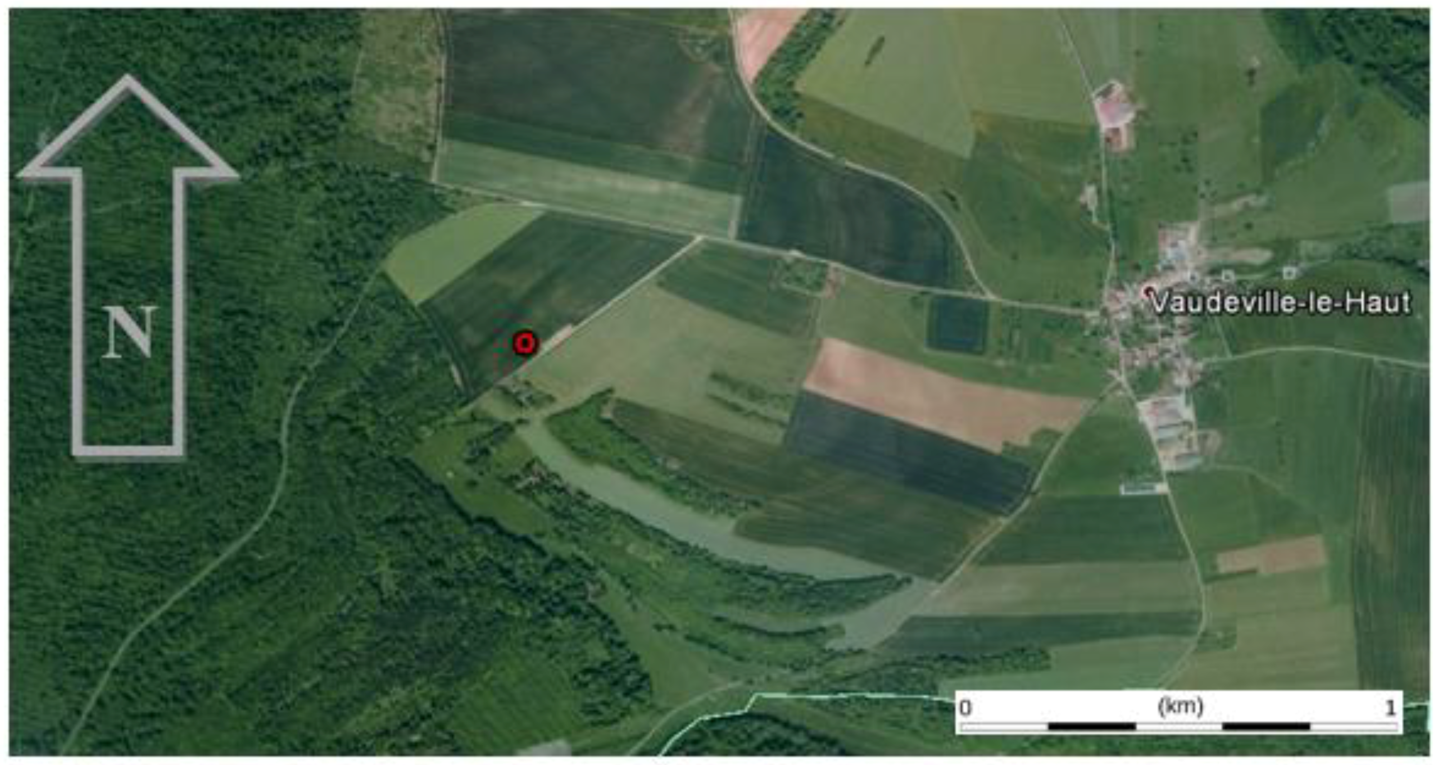
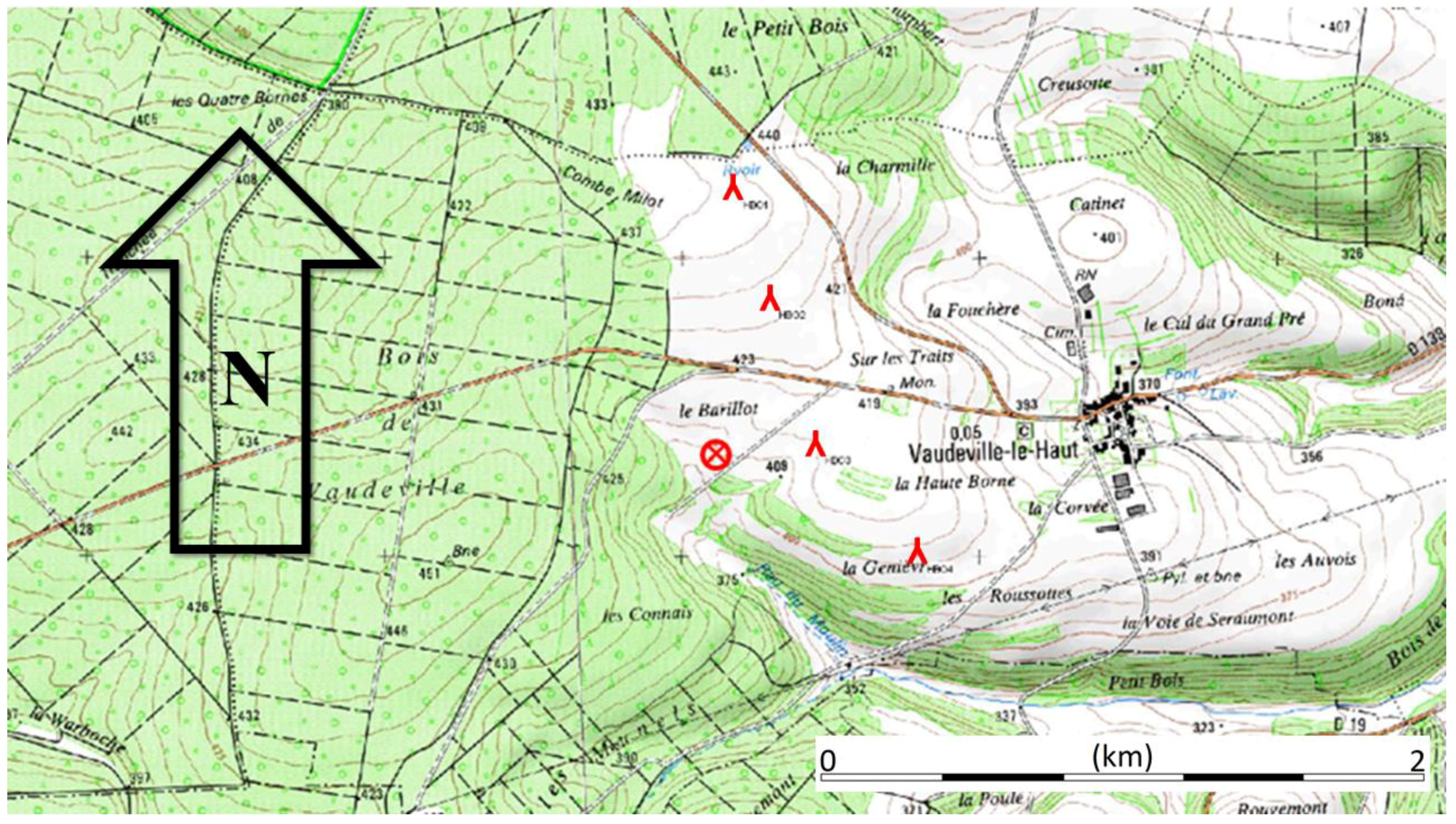
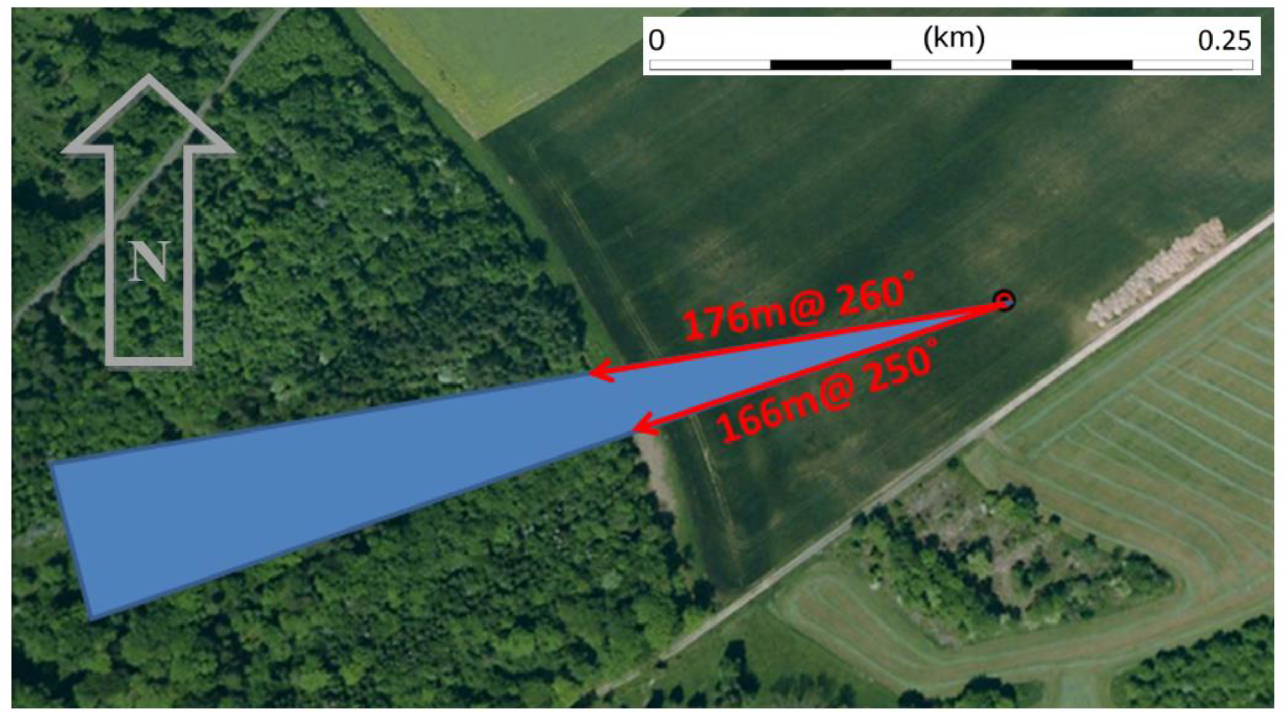
2. Validation Data
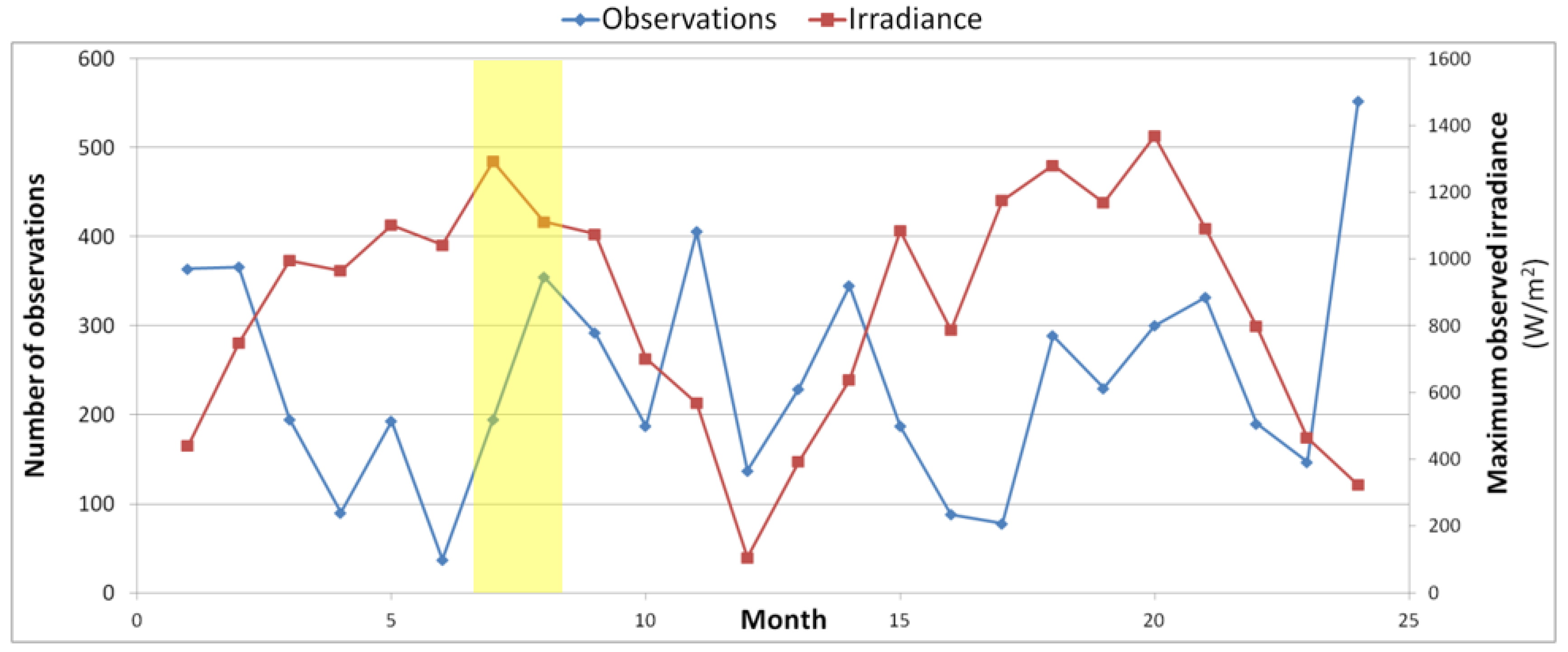
2.1. Wind Speed Data
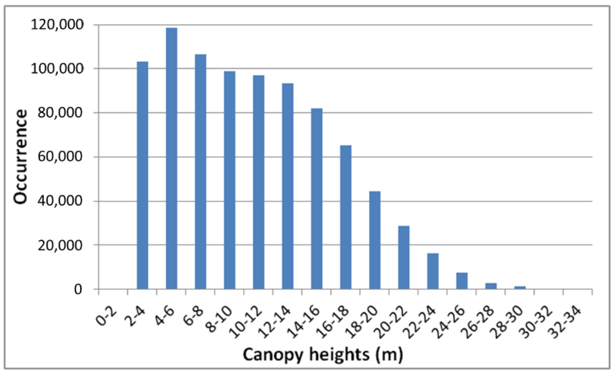
2.2. Canopy Height Data
3. CFD Modelling
3.1. Model Equations
3.2. Boundary Conditions
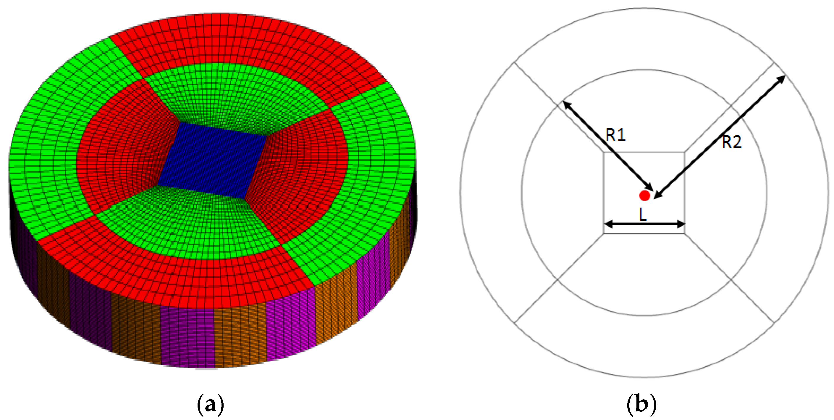
3.3. Domain Description
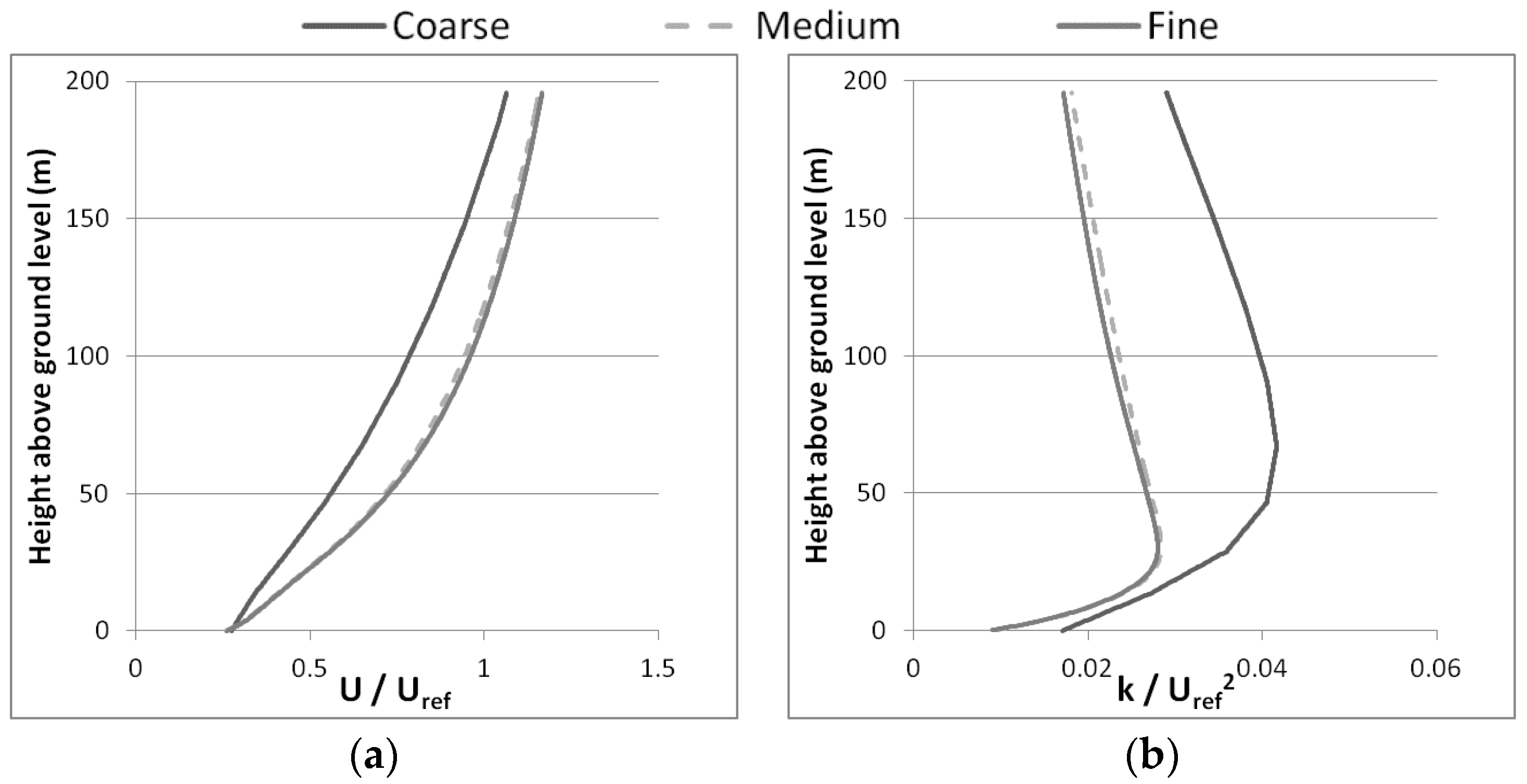
3.4. Mesh Sensitivity
4. Neutral Simulations
4.1. Process
- Reference height, Zref
- Reference velocity, Uref
- Canopy loss coefficient, Lx: Variable hc
- Canopy loss coefficient, Lx: Constant hc
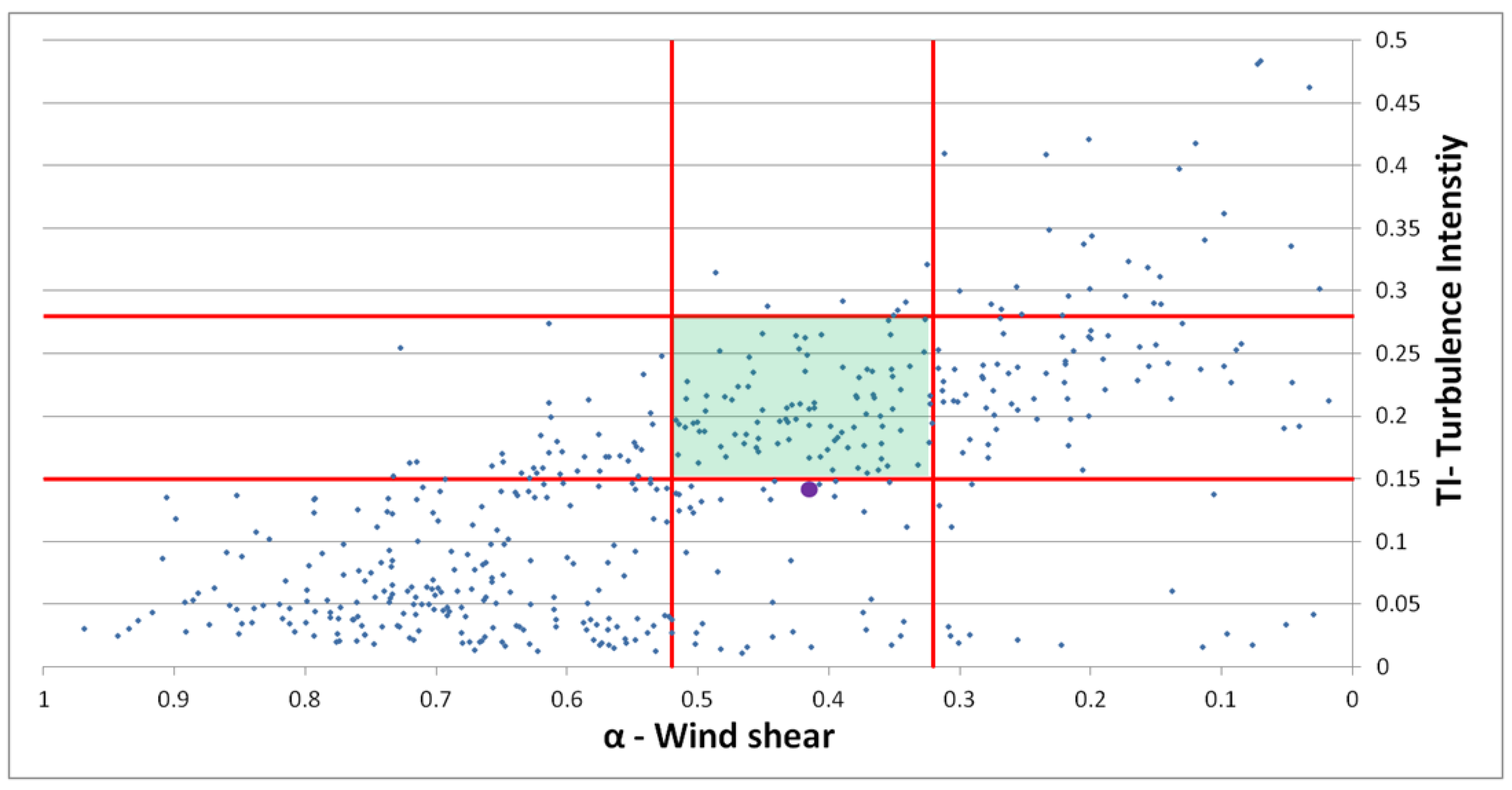
4.2. Results
4.2.1. Reference Height, Zref and Reference Velocity, Uref
4.2.2. Canopy Loss Coefficient, Lx: Variable hc
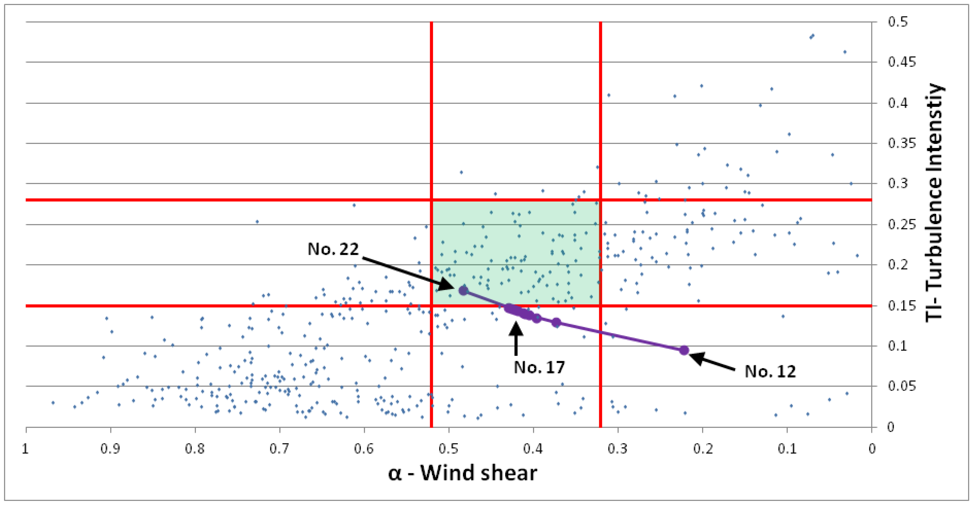
4.2.3. Canopy Loss Coefficient, Lx: Constant hc
4.3. Discussion
5. Stable Simulations
5.1. Process
5.2. Results
5.3. Discussion
6. Unstable Simulations
7. Conclusions
Author Contributions
Funding
Conflicts of Interest
Nomenclature
| Symbol | Definition | Units |
| Leaf area density at height z | m−1 | |
| Canopy drag coefficient | dimensionless | |
| Turbulence model constants for SST model | dimensionless | |
| Turbulence model constants specific to forest canopy model | dimensionless | |
| Fluid specific heat capacity at constant pressure | J/(kg K) | |
| Wall distance functions in SST model | dimensionless | |
| Forestry switch | dimensionless | |
| Buoyancy force per unit volume in the i-direction | kg/(m2 s2) | |
| Coriolis force per unit volume in the i-direction | kg/(m2 s2) | |
| Drag force per unit volume in the i-direction | kg/(m2 s2) | |
| Momentum flux | N/m2 | |
| Coriolis parameter | s−1 | |
| Gravity acceleration | m/s2 | |
| Equivelent sand grain roughness | m | |
| Turbulence kinetic energy | m2/s2 | |
| Pressure | Pa | |
| Shear turbulence production per unit volume | kg/(m s3) | |
| Buoyancy turbulence production per unit volume | kg/(m s3) | |
| Buoyancy production term for eddy frequency, per unit volume | kg/(m3 s2) | |
| Turbulence dissipation source per unit volume | kg/(m s4) | |
| Turbulence kinetic energy production from forestry drag, per unit volume | kg/(m s3) | |
| Eddy frequency production from forestry drag, per unit volume | kg/(m3 s2) | |
| Time | s | |
| Turbulence intensity | dimensionless | |
| Modulus of the windspeed | m/s | |
| 10 min mean wind speed | m/s | |
| Velocity at reference height z | m/s | |
| Wind speed in the i-direction, j-direction | m/s | |
| Geostrophic wind speed in the i-direction | m/s | |
| 10 min mean wind speed at 40 m, 80 m | m/s | |
| Friction velocity | m/s | |
| Spatial coordinate in i-direction | m | |
| Spatial coordinate in i-direction | m | |
| Shear exponent factor | dimensionless | |
| Thermal expansion coefficient | K−1 | |
| ,, | Turbulent Prandtl number for momentum, temperature, and | dimensionless |
| Standard deviation of wind speed over 10 min, sampled at a rate of 1 Hz | m/s | |
| Turbulence disspation rate | m2/s3 | |
| Potential temperature | K | |
| Von Karmen constant | dimensionless | |
| Fluid conductivity | W/(m K) | |
| Fluid viscosity | kg/(m s) | |
| Eddy viscosity | kg/(m s) | |
| Fluid density | kg/m−3 | |
| Turbulence eddy frequency | s−1 |
References
- Mortensen, N.; Jørgensen, H. Comparative Resource and Energy Yield Assessment Procedures. In Proceedings of the European Wind Energy Association Technology Workshop: Resource Assessment, Dublin, Ireland, 26 June 2013. [Google Scholar]
- Brower, M.C.; Vidal, J.; Beaucage, P. A Performance comparison of four numerical wind flow modeling systems. In Proceedings of the European Wind Energy Association Annual Conference, Barcelona, Spain, 10–13 March 2014. [Google Scholar]
- Desmond, C.; Watson, S. A study of stability effects in forested terrain. J. Phys. Conf. Ser. 2014, 555, 012027. [Google Scholar] [CrossRef]
- Brunet, Y.; Irvine, R. The control of coherent eddies in vegetation canopies: Streamwise structures spacing, canopy shear scale and atmospheric stability. Bound. Layer Meteorol. 2000, 94, 139–163. [Google Scholar] [CrossRef]
- Morse, A.P.; Gardiner, B.A.; Marshall, B.J. Mechanisms controlling turbulence development across a forest edge. Bound. Layer Meteorol. 2001, 130, 227–251. [Google Scholar] [CrossRef]
- Chaudhari, A.; Conan, B.; Aubrun, S.; Hellsten, A. Numerical study of how stable stratification affects turbulence instabilities above a forest cover: Application to wind energy. J. Phys. Conf. Ser. 2016, 753, 032037. [Google Scholar] [CrossRef]
- Desmond, C.; Watson, S.; Hancock, P. Modelling the wind energy resources in complex terrain and atmospheres. 5 Numerical simulation and wind tunnel investigation of non-neutral forest canopy flows. J. Wind Eng. Ind. Aerodyn. 2017, 166, 48–60. [Google Scholar] [CrossRef]
- Texier, O.; Clarenc, T.; Bezault, C.; Girard, N.; Degelder, J. Integration of atmospheric stability in wind power assessment through CFD modeling. In Proceedings of the EWEC 2010, Warsaw, Poland, 20–23 April 2010. [Google Scholar]
- Andersen, H.E.; Mcgaughey, R.J.; Reutebuch, S.E. Assessing the influence of flight parameters, interferometric processing, slope and canopy density on the accuracy of X-band IFSAR-derived forest canopy height models. Int. J. Remote Sens. 2008, 29, 1495–1510. [Google Scholar] [CrossRef]
- Desmond, C.; Watson, S.; Aubrun, S.; Avila, S.; Hancock, P.; Sayer, A. A study on the inclusion of forest canopy morphology data in numerical simulations for the purpose of wind resource assessment. J. Wind Eng. Ind. Aerodyn. 2014, 126, 24–37. [Google Scholar] [CrossRef]
- Menter, F. Two-Equation Eddy-Viscosity Transport Turbulence Model for Engineering Applications. AIAA J. 1994, 32, 1598–1605. [Google Scholar] [CrossRef]
- McCormick, S.; Montavon, C.; Jones, I.; Staples, C.; Sinai, Y. Atmospheric boundary layer. In Boundary Layer Conditions and Profiles; WindModeller Manuals; ANSYS: Cannonsburg, PA, USA, 2012. [Google Scholar]
- Svensson, U.; Haggkvist, H. A two-equation turbulence model for canopy flows. J. Wind Eng. Ind. Aerodyn. 1990, 35, 201–211. [Google Scholar] [CrossRef]
- Lopes da Costa, J.C.P. Atmospheric Flow over Forested and Non-Forested Complex Terrain. Ph.D. Thesis, University of Porto, Porto, Portugal, 2007. [Google Scholar]
- Katul, G.; Mahrt, L.; Poggi, D.; Sanz, C. One and two equation models for canopy turbulence. Bound. Layer Meteorol. 2003, 113, 81–109. [Google Scholar] [CrossRef]
- Sogachev, A. A note on two equation closure modelling of canopy flow. Bound. Layer Meteorol. 2009, 130, 423–435. [Google Scholar] [CrossRef]
- Lechner, R.; Menter, F.R. Development of a Rough Wall Boundary Condition for ω-Based Turbulence Models; Technical Report ANSYS/TR-04-04; ANSYS CFX: Otterfing, Germany, 2004. [Google Scholar]
- U.S. Government Printing Office. U.S. Standard Atmosphere, 1962; U.S. Government Printing Office: Washington, DC, USA, 1962.
- Richards, P.J.; Hoxey, R.P. Appropriate boundary conditions for computational wind engineering models using the k-ϵ turbulence model. J. Wind Eng. Ind. Aerodyn. 1993, 46, 145–153. [Google Scholar] [CrossRef]
- Zilitinkevich, S.; Johansson, P.E.; Mironov, D.V.; Baklanov, A. A similarity-theory model for wind profile and resistance law in stably stratified planetary boundary layers. J. Wind Eng. Ind. Aerodyn. 1998, 74–76, 209–218. [Google Scholar] [CrossRef]
- Zilitinkevich, S.S.; Mironov, D.V. A Multi-Limit Formulation for the Equilibrium Depth of a Stably Stratified Boundary Layer. Bound. Layer Meteorol. 1996, 81, 325–351. [Google Scholar] [CrossRef]
- Montavon, C. Simulation of Atmospheric Flows over Complex Terrain for Wind Power Potential Assessment. Ph.D. Thesis, École Polytechnique Fédérale de Lausanne, Lausanne, Switzerland, 1998. [Google Scholar]
- Werner, M. Shuttle Radar Topography Mission (SRTM) Mission Overview. Frequenz 2001, 55, 75–79. [Google Scholar] [CrossRef]
- Burton, T.; Jenkins, N.; Sharpe, D.; Bossanyi, E. Wind Energy Handbook, 2nd ed.; Wiley: Hoboken, NJ, USA, 2011. [Google Scholar]
- Amiro, B.D. Drag coefficients and turbulence spectra within three boreal forest canopies. Bound. Layer Meterol. 1990, 52, 227–246. [Google Scholar] [CrossRef]
- Banerjee, T.; Katul, G.; Fontan, S.; Poggi, D.; Kumar, M. Mean flow near edges and within cavities situated inside dense canopies. Bound. Layer Meterol. 2013, 149, 19–41. [Google Scholar] [CrossRef]
- Silva Lopes, A.; Palma, J.M.L.M.; Viana Lopes, J. Improving a two equation turbulence model for canopy flows using Large Eddy Simulation. J. Bound. Layer Meterol. 2013, 149, 231–257. [Google Scholar] [CrossRef]
- Segalini, A.; Nakamure, T.; Fukagate, K. A linearized k-Epsilon Model of Forest Canopies and Clearing. J. Bound. Layer Meterol. 2016, 161, 439–460. [Google Scholar] [CrossRef]
- Lopes da Costa, J.C.; Castro, F.A.; Santos, C.S. Large-Eddy simulation of thermally stratified forest canopy flows for wind energy studies purposes. In Proceedings of the 4th International Conference on Energy and Environment Research (ICEER), Porto, Portugal, 17–20 July 2017. [Google Scholar]


| Height (m) | Sensor 1 | Sensor 2 | Sensor 3 |
|---|---|---|---|
| 80 | Temperature sensor (PT 100, SKS Sensors, Vantaa, Finland) | 3D Sonic anemometer (Metek USA-1) | Cup Anemometer (Thies First class, Thies, Göttingen, Germany) |
| 70 | Wind vane (Thies compact) | - | - |
| 60 | Temperature sensor (PT 100) | 3D Sonic anemometer (Metek USA-1) | - |
| 40 | Temperature sensor (PT 100) | 3D Sonic anemometer (Metek USA-1) | - |
| 10 | Temperature sensor (PT 100) | 3D Sonic anemometer (Metek USA-1) | - |
| 3 | Temperature & Humidity (CS215) | Pyranometer (CMP6, Kipp & Zonen, Delft, The Neterlands) | - |
| 1 | Pluviometer | - | - |
| -1 | Temperature sensor (PT 100) | - | - |
| Stability Class | Time & Date |
|---|---|
| Stable | 19:40 13 July 2010 |
| Neutral | 23:40 17 August 2010 |
| Unstable | 12:00 10 August 2010 |
| Constant | Value |
|---|---|
| 0.17 | |
| 3.37 | |
| 0.9 | |
| 0.9 |
| Mesh | Maximum Cell Size | Control Volumes | Nodes | CPU Time | |
|---|---|---|---|---|---|
| Hz | Vt | ||||
| Coarse | 100 m | 100 m | 87,696 | 93,478 | 5 min |
| Medium | 20 m | 50 m | 2,149,056 | 2,215,626 | 60 min |
| Fine | 10 m | 25 m | 13,418,460 | 13,638,322 | 480 min |
| Simulation No. | CFD Settings | CFD Output | |||||
|---|---|---|---|---|---|---|---|
| Zref (m) | Uref (m/s) | Lx (m−1) | Cμ | hc (m) | α | TI | |
| 1 | 40 | 6.5 | 0.05 | 0.09 | Variable | 0.415 | 0.142 |
| 2 | 60 | 6.5 | 0.05 | 0.09 | Variable | 0.415 | 0.142 |
| 3 | 80 | 6.5 | 0.05 | 0.09 | Variable | 0.415 | 0.142 |
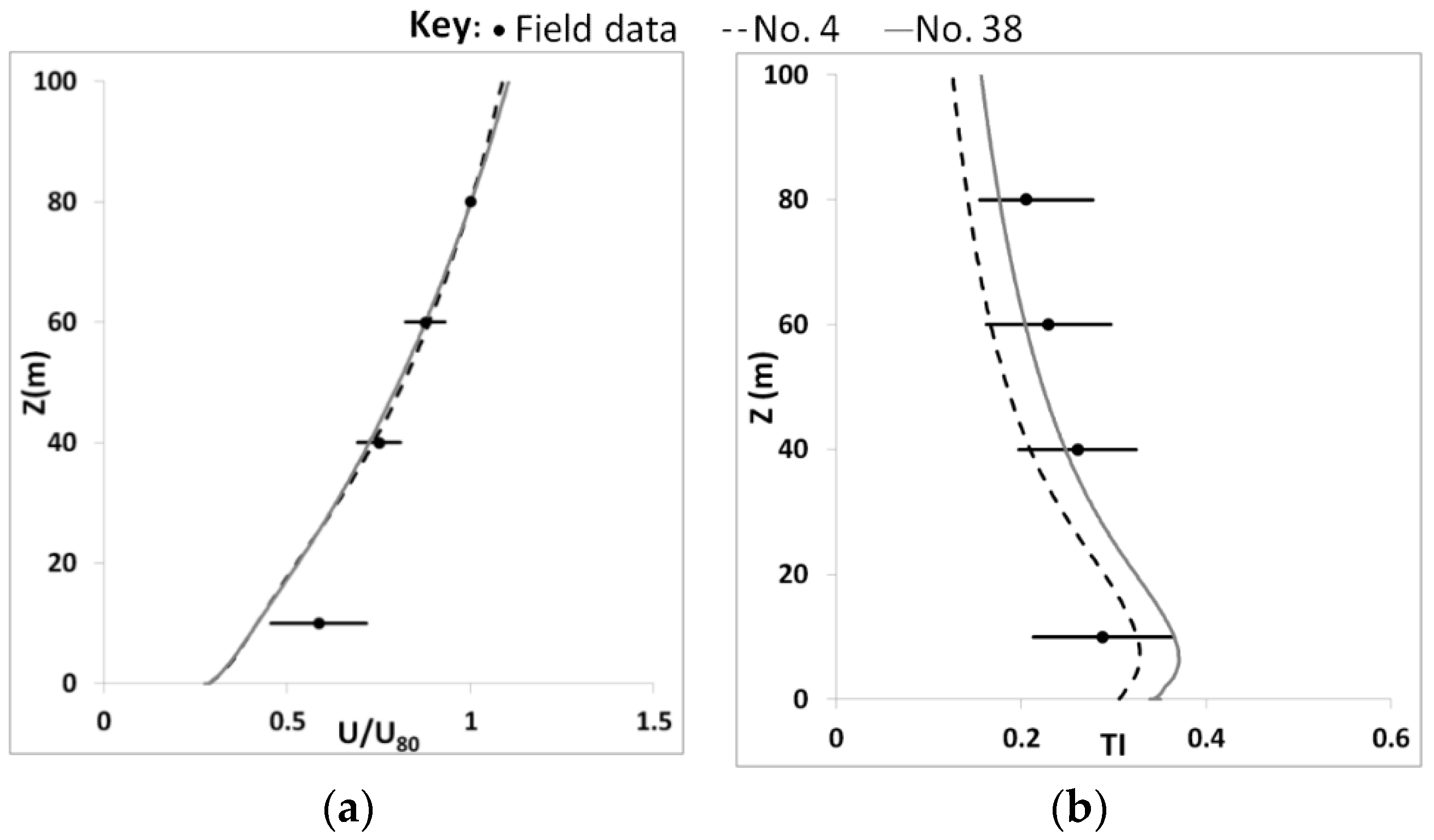
| 4 | 100 | 6.5 | 0.05 | 0.09 | Variable | 0.415 | 0.142 |
| 5 | 500 | 6.5 | 0.05 | 0.09 | Variable | 0.415 | 0.142 |
| Simulation No. | CFD Settings | CFD Output | |||||
|---|---|---|---|---|---|---|---|
| Zref (m) | Uref (m/s) | Lx (m−1) | Cμ | hc (m) | α | TI | |
| 6 | 100 | 5 | 0.05 | 0.09 | Variable | 0.418 | 0.141 |
| 7 | 100 | 5.5 | 0.05 | 0.09 | Variable | 0.418 | 0.141 |
| 8 | 100 | 6 | 0.05 | 0.09 | Variable | 0.417 | 0.141 |
| 9 | 100 | 7 | 0.05 | 0.09 | Variable | 0.417 | 0.141 |
| 10 | 100 | 13 | 0.05 | 0.09 | Variable | 0.418 | 0.142 |
| 11 | 100 | 20 | 0.05 | 0.09 | Variable | 0.418 | 0.142 |
| Simulation No. | CFD Settings | CFD Output | |||||
|---|---|---|---|---|---|---|---|
| Zref (m) | Uref (m/s) | Lx (m−1) | Cμ | hc (m) | α | TI | |
| 12 | 100 | 6.5 | 0.001 | 0.09 | Variable | 0.223 | 0.095 |
| 13 | 100 | 6.5 | 0.01 | 0.09 | Variable | 0.373 | 0.129 |
| 14 | 100 | 6.5 | 0.02 | 0.09 | Variable | 0.397 | 0.135 |
| 15 | 100 | 6.5 | 0.03 | 0.09 | Variable | 0.405 | 0.138 |
| 16 | 100 | 6.5 | 0.04 | 0.09 | Variable | 0.411 | 0.140 |
| 17 | 100 | 6.5 | 0.045 | 0.09 | Variable | 0.413 | 0.141 |
| 18 | 100 | 6.5 | 0.06 | 0.09 | Variable | 0.420 | 0.144 |
| 19 | 100 | 6.5 | 0.07 | 0.09 | Variable | 0.423 | 0.145 |
| 20 | 100 | 6.5 | 0.08 | 0.09 | Variable | 0.426 | 0.146 |
| 21 | 100 | 6.5 | 0.09 | 0.09 | Variable | 0.430 | 0.148 |
| 22 | 100 | 6.5 | 0.5 | 0.09 | Variable | 0.484 | 0.169 |
| Simulation No. | CFD Settings | CFD Output | |||||
|---|---|---|---|---|---|---|---|
| Zref (m) | Uref (m/s) | Lx (m−1) | Cμ | hc (m) | α | TI | |
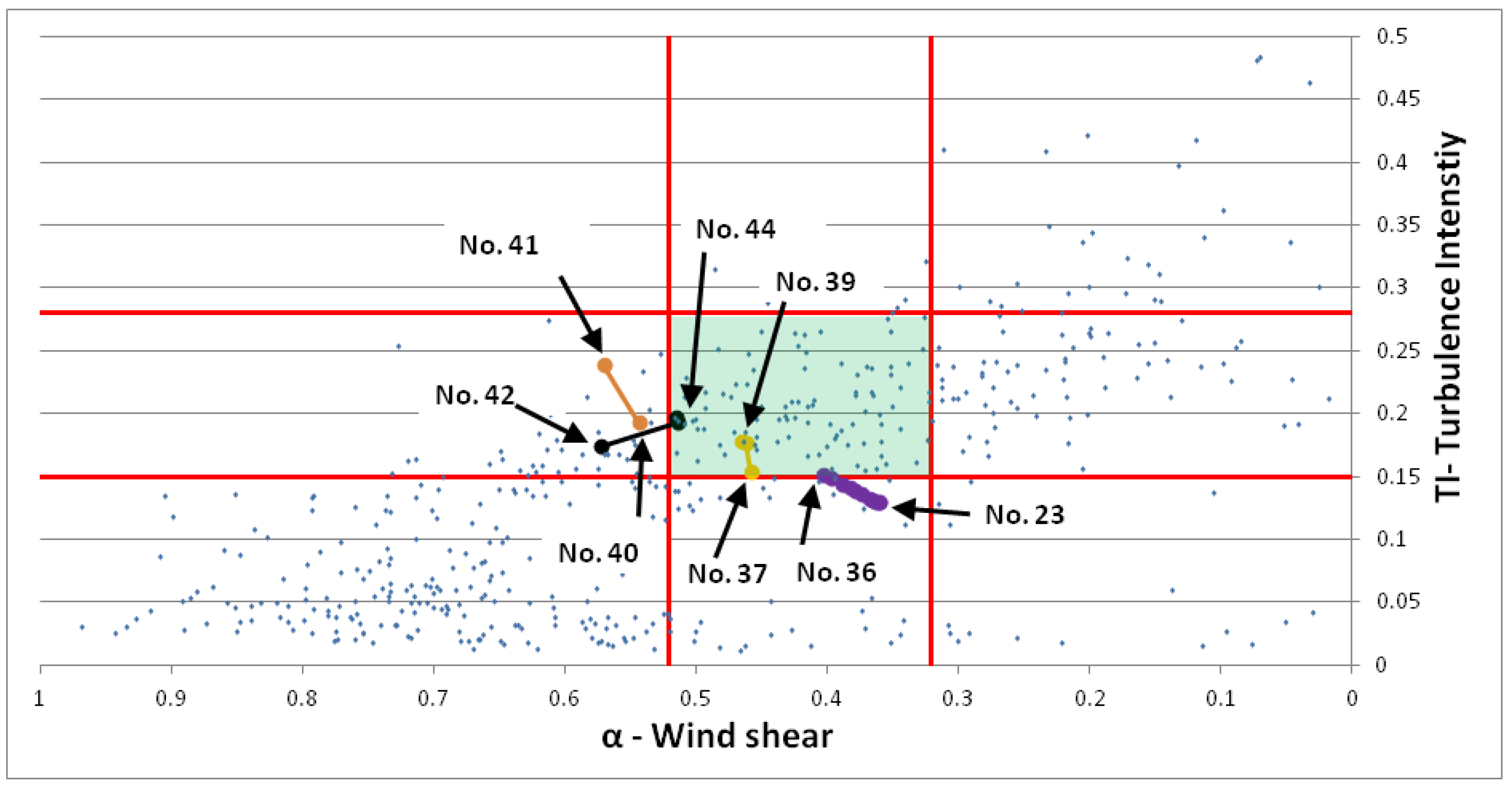
| 23 | 100 | 6.5 | 0.02 | 0.09 | 11 | 0.360 | 0.130 |
| 24 | 100 | 6.5 | 0.03 | 0.09 | 11 | 0.360 | 0.130 |
| 25 | 100 | 6.5 | 0.04 | 0.09 | 11 | 0.363 | 0.130 |
| 26 | 100 | 6.5 | 0.05 | 0.09 | 11 | 0.365 | 0.131 |
| 27 | 100 | 6.5 | 0.06 | 0.09 | 11 | 0.368 | 0.133 |
| 28 | 100 | 6.5 | 0.09 | 0.09 | 11 | 0.374 | 0.136 |
| 29 | 100 | 6.5 | 0.12 | 0.09 | 11 | 0.379 | 0.138 |
| 30 | 100 | 6.5 | 0.15 | 0.09 | 11 | 0.383 | 0.141 |
| 31 | 100 | 6.5 | 0.2 | 0.09 | 11 | 0.389 | 0.144 |
| 32 | 100 | 6.5 | 0.3 | 0.09 | 11 | 0.397 | 0.148 |
| 33 | 100 | 6.5 | 0.4 | 0.09 | 11 | 0.404 | 0.151 |
| 34 | 100 | 6.5 | 0.6 | 0.09 | 11 | 0.412 | 0.156 |
| 35 | 100 | 6.5 | 0.7 | 0.09 | 11 | 0.415 | 0.158 |
| 36 | 100 | 6.5 | 0.8 | 0.09 | 11 | 0.414 | 0.158 |
| Simulation No. | CFD Settings | CFD Output | |||||
|---|---|---|---|---|---|---|---|
| Zref (m) | Uref (m/s) | Lx (m−1) | Cμ | hc (m) | α | TI | |
| 37 | 100 | 6.5 | 0.05 | 0.09 | 20 | 0.458 | 0.154 |
| 38 | 100 | 6.5 | 0.7 | 0.09 | 20 | 0.462 | 0.176 |
| 39 | 100 | 6.5 | 0.9 | 0.09 | 20 | 0.465 | 0.179 |
| Simulation No. | CFD Settings | CFD Output | |||||
|---|---|---|---|---|---|---|---|
| Zref (m) | Uref (m/s) | Lx (m−1) | Cμ | hc (m) | α | TI | |
| 40 | 100 | 6.5 | 0.05 | 0.09 | 25 | 0.544 | 0.193 |
| 41 | 100 | 6.5 | 0.9 | 0.09 | 25 | 0.570 | 0.238 |
| Simulation No. | CFD Settings | CFD Output | |||||
|---|---|---|---|---|---|---|---|
| Zref (m) | Uref (m/s) | Lx (m−1) | Cμ | hc (m) | α | TI | |
| 42 | 100 | 6.5 | 0.05 | 0.09 | 30 | 0.572 | 0.174 |
| 43 | 100 | 6.5 | 0.7 | 0.09 | 30 | 0.514 | 0.193 |
| 44 | 100 | 6.5 | 0.9 | 0.09 | 30 | 0.515 | 0.197 |
| Simulation No. | Floor Temperature Difference from Ambient (Kelvin) | CFD Output | ||
|---|---|---|---|---|
| α | TI | Time (min) | ||
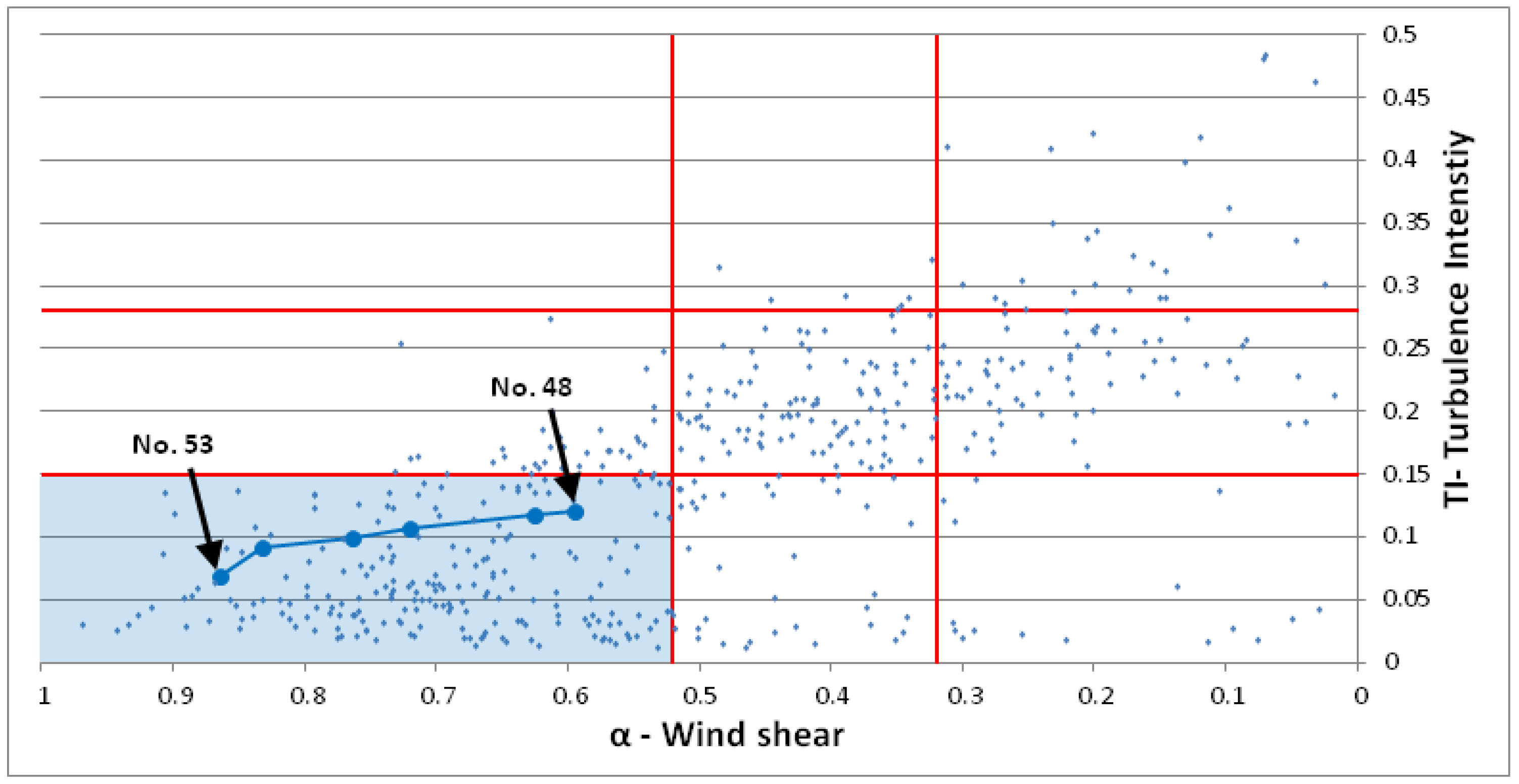
| 48 | −0.5 | 0.594 | 0.120 | 800 |
| 49 | −1 | 0.626 | 0.117 | 828 |
| 50 | −5 | 0.720 | 0.107 | 1088 |
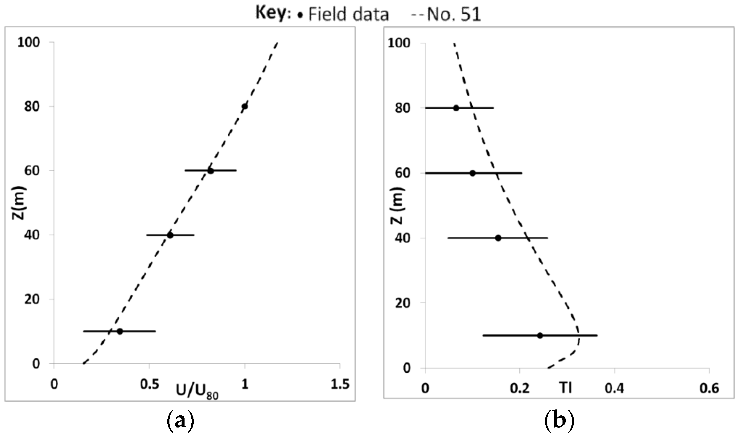
| 51 | −10 | 0.764 | 0.099 | 2204 |
| 52 | −25 | 0.833 | 0.092 | 2434 |
| 53 | −50 | 0.864 | 0.068 | 2574 |
© 2018 by the authors. Licensee MDPI, Basel, Switzerland. This article is an open access article distributed under the terms and conditions of the Creative Commons Attribution (CC BY) license (http://creativecommons.org/licenses/by/4.0/).
Share and Cite
Desmond, C.J.; Watson, S.; Montavon, C.; Murphy, J. Modelling Uncertainty in t-RANS Simulations of Thermally Stratified Forest Canopy Flows for Wind Energy Studies. Energies 2018, 11, 1703. https://doi.org/10.3390/en11071703
Desmond CJ, Watson S, Montavon C, Murphy J. Modelling Uncertainty in t-RANS Simulations of Thermally Stratified Forest Canopy Flows for Wind Energy Studies. Energies. 2018; 11(7):1703. https://doi.org/10.3390/en11071703
Chicago/Turabian StyleDesmond, Cian J., Simon Watson, Christiane Montavon, and Jimmy Murphy. 2018. "Modelling Uncertainty in t-RANS Simulations of Thermally Stratified Forest Canopy Flows for Wind Energy Studies" Energies 11, no. 7: 1703. https://doi.org/10.3390/en11071703
APA StyleDesmond, C. J., Watson, S., Montavon, C., & Murphy, J. (2018). Modelling Uncertainty in t-RANS Simulations of Thermally Stratified Forest Canopy Flows for Wind Energy Studies. Energies, 11(7), 1703. https://doi.org/10.3390/en11071703