Fault Analysis Method Considering Dual-Sequence Current Control of VSCs under Unbalanced Faults

Abstract

Voltage source converters (VSCs) are able to provide both positive- and negative-sequence short circuit currents under unbalanced faults. Their short circuit responses can be significantly different from those of conventional synchronous generators. This paper developed a static fault analysis method by considering dual-sequence current control of VSCs under unbalanced faults where VSCs are treated as voltage-dependent current sources in both positive- and negative-sequence networks. Since the control strategy of VSCs varies, flexible parameters are included in the model to reflect their diverse short circuit behaviours. The proposed method is verified through a modified IEEE 9-bus system and a simplified western Danish power system with real time simulations. This analytical method can be used to help understand and evaluate the impact of dual-sequence current control of VSCs on future converter-dominated power systems.

1. Introduction

With proliferated renewable energy integration and the gradual retirement of conventional generation units, power systems are undergoing significant changes in regard to their generation mixes. Voltage source converters are widely utilized in power systems, such as Type-IV wind power plants, photovoltaic power plants and high-voltage direct current (HVDC) connections because of their control flexibility [1]. The different national and international grid codes require that converters shoule be capable of staying connected to the network and providing a short circuit current under grid fault conditions [2,3,4]. However, the short circuit response of a current-controlled voltage source converter (VSC) is mainly governed by its control system and can be significantly different from that of a synchronous generator. Under grid unbalanced faults, a VSC can be controlled to provide both positive- and negative-sequence currents with advanced control techniques [5]. Therefore, the conventional method [6] for static fault analysis is inadequate as it does not take the dual-sequence current control of VSCs into consideration.

Under grid unbalanced faults, a VSC is conventionally controlled to maintain a balanced three-phase short circuit current, and the negative-sequence current references are always set to zero [7,8]. In recent years, the potential of VSCs to provide positive- and negative-sequence short circuit currents simultaneously has received increasing attention [9,10,11,12,13,14,15]. In [9,10], a negative-sequence current was injected to help reduce the active power or reactive power oscillations. The focus was on the VSC itself and its impact on the grid was not investigated. The work in [11,12] aimed to regulate the grid phase-voltage under unbalanced fault conditions to comply with pre-defined voltage limits. Multi-objective control strategies were proposed in [13,14,15] considering the characteristics of VSC output powers and their capability to regulate grid voltage at the same time. However, these studies focused on the control of a single VSC connected to an ideal voltage source, without considering application to a larger power system. The studies in [16,17,18,19] investigated the impact of dual-sequence short circuit currents from a single VSC on grid voltages using dynamic simulations. Even though dynamic simulations can exhibit transient behaviours and give accurate results, they are not able to analytically calculate the short circuit currents or the system’s retained voltage. Moreover, if different control strategies are to be evaluated and there are multiple VSCs in the system, the modelling work for dynamic simulations can become quite time-consuming. Modern grid codes have started to define the negative-sequence current injection requirements for VSCs [4,19] during unbalanced faults. Therefore, a static fault analysis method that considers the dual-sequence current control of VSCs under unbalanced faults is needed.

In order to represent a VSC mathematically, a sequence-component-based VSC model was proposed in [20]. In this model, the converter is either treated as an ideal voltage source or as a constant power source depending on the operation mode. This model is mainly for power flow analysis and is not suitable for the representation of a VSC for fault analysis. The work in [21] used VSCs as constant current sources in the positive-sequence networks, whereas negative-sequence short circuit currents were not considered. In [22], the concept of fault current distribution coefficients was proposed to express the fault current contributions from VSCs seen at the fault locations. This method assumes constant grid voltages and can only be applied to small-scale, grid-connected microgrids.

The studies in [23,24,25,26] treated VSCs as current sources in a phasor domain. Fault analyses were conducted by performing power flow analyses of the faulted network using Gauss–Siedel or Newton–Raphson algorithms. These power-flow-based methods are solely applied to distribution networks based on the assumption that the main grid can be considered to be an infinite bus whose voltage does not drop under fault conditions. As a result, the main grid can be identified as the slack bus for the power flow analysis. However, these methods cannot be extended to transmission networks where such kind of infinite buses does not really exist.

In addition, the above power-flow-based methods are circumscribed when it comes to unbalanced faults. It was assumed in [25,26] that the VSCs do not contribute any negative-sequence current under grid unbalanced faults. Consequently, the passive negative- and zero-sequence networks were combined and modeled as an equivalent impedance shunt-connected at the fault location. If VSCs are controlled to also provide a negative-sequence short circuit current, the negative-sequence network will not be passive anymore and power-flow-based methods become insufficient. Similarly, the studies in [27,28] based on the bus impedance matrix also assumed that the negative-sequence network is passive, which does not accommodate the dual-sequence current control of VSCs either.

This paper develops a static fault analysis method that considers dual-sequence current control of VSCs under unbalanced faults. It treats VSCs as voltage-dependent current sources in both positive- and negative-sequence networks. Flexible parameters are included in the VSC model to represent various control strategies. The proposed method is capable of taking the dual-sequence short circuit currents from multiple VSCs into account. The calculation results are verified through a comparison with the simulation results from Real Time Digital Simulator (RTDS). As an application, the method is used to help explain a phenomenon that the system does not have a stable fault response when the share of negative-sequence reactive power from VSCs is high or when the system has a low short-circuit power. This phenomenon has not been revealed by previous studies. The proposed method can be utilized to help understand and evaluate the impact of dual-sequence current control of VSCs on the system.

2. Fault Analysis Method

2.1. Dual-Sequence Current Control

For a three-phase, three-wire VSC system, the zero-sequence components are not present. Therefore, the instantaneous active and reactive powers measured at the point of common coupling (PCC) can be expressed by [29]:

$$\begin{array}{cc}\hfill p& =\stackrel{P^{+}}{\overbrace{{\mathbf{v}}^{+}·{\mathbf{i}}^{+}}}+\stackrel{P^{-}}{\overbrace{{\mathbf{v}}^{-}·{\mathbf{i}}^{-}}}+\stackrel{\tilde{P}}{\overbrace{{\mathbf{v}}^{+}·{\mathbf{i}}^{-}+{\mathbf{v}}^{-}·{\mathbf{i}}^{+}}}\hfill \end{array}$$

(1)

$$\begin{array}{cc}\hfill q& =\stackrel{Q^{+}}{\overbrace{{\mathbf{v}}_{\perp }^{+}·{\mathbf{i}}^{+}}}+\stackrel{Q^{-}}{\overbrace{{\mathbf{v}}_{\perp }^{-}·{\mathbf{i}}^{-}}}+\stackrel{\tilde{Q}}{\overbrace{{\mathbf{v}}_{\perp }^{+}·{\mathbf{i}}^{-}+{\mathbf{v}}_{\perp }^{-}·{\mathbf{i}}^{+}}}\hfill \end{array}$$

(2)

where $\mathbf{v}={\left[v_a{v}_b{v}_c\right]}^T$ and $\mathbf{i}={\left[i_a{i}_b{i}_c\right]}^T$ are the voltage and current vectors at the PCC; the subscript “⊥” represents a 90°-lagging version of the original vector; the superscripts “+” and “−” refer to the positive- and negative-sequence components; the operator “·” refers to the dot product of vectors; $P^{+}$ and $Q^{+}$ are positive-sequence powers originating from positive-sequence components, while $P^{-}$ and $Q^{-}$ are negative-sequence powers resulting from negative-sequence components; $\tilde{P}$ and $\tilde{Q}$ are the oscillating power terms, whose average value is zero.

The dual-sequence current control strategy of a VSC mainly depends on how its current references are generated [5]. Even though the current references can be formulated in various ways, a common feature of these strategies is that they can feed positive- and negative-sequence short circuit currents simultaneously. Therefore, the current references can be decomposed into positive- and negative-sequence components, and can be expressed by Equations (3) and (4) in a more general form [30]:

$$\begin{array}{cc}\hfill {\mathbf{i}}^{+}& =a\frac{P^{ref}}{{\left|{\mathbf{v}}^{+}\right|}^2}{\mathbf{v}}^{+}+c\frac{Q^{ref}}{{\left|{\mathbf{v}}^{+}\right|}^2}{\mathbf{v}}_{\perp }^{+}\hfill \end{array}$$

(3)

$$\begin{array}{cc}\hfill {\mathbf{i}}^{-}& =b\frac{P^{ref}}{{\left|{\mathbf{v}}^{-}\right|}^2}{\mathbf{v}}^{-}+d\frac{Q^{ref}}{{\left|{\mathbf{v}}^{-}\right|}^2}{\mathbf{v}}_{\perp }^{-}\hfill \end{array}$$

(4)

where a, b, c and d are the four factors that determine the control strategy; $P^{ref}$ and $Q^{ref}$ are the active and reactive power references, respectively. By substituting Equations (3) and (4) into Equations (1) and (2), the instantaneous powers can be simplified as

$$\begin{array}{cc}\hfill p& =\stackrel{P^{+}}{\overbrace{a{P}^{ref}}}+\stackrel{P^{-}}{\overbrace{b{P}^{ref}}}+\tilde{P}\hfill \end{array}$$

(5)

$$\begin{array}{cc}\hfill q& =\stackrel{Q^{+}}{\overbrace{c{Q}^{ref}}}+\stackrel{Q^{-}}{\overbrace{d{Q}^{ref}}}+\tilde{Q}.\hfill \end{array}$$

(6)

Since the average value of the oscillating power terms is zero, $a+b=1$ and $c+d=1$ have to be satisfied so that the output powers from the VSC satisfy its power references [30]. This indicates that the control strategies can be characterized by two factors, a and c, which represent the share of the positive-sequence active and reactive powers, respectively. Therefore, different control strategies can principally be considered to be different combinations of the sequence output powers. In the following text, current references with Equations (3) and (4) will be used to represent the short circuit response of VSC-based sources in the proposed fault analysis method.

2.2. Algorithm

For balanced fault analysis using the conventional method, changes in the network voltages caused by a fault are equivalent to those caused by a voltage source at the fault terminal when all other voltage sources are short-circuited. For unbalanced faults, the analysis is conducted by algebraically manipulating the Thevenin equivalent circuits of sequence networks, as seen from the fault location, according to the fault types. However, the conventional method cannot be directly applied if a VSC exists in the system. When Equations (3) and (4) are used, both positive- and negative-sequence networks are shown to be active, while the conventional method assumes the negative-sequence network is passive. In addition, the formation of Equations (3) and (4) indicates that VSCs should be treated as voltage-dependent current sources whose magnitudes and phases rely on the voltages at the PCC. However, current injections from VSCs can also alter the PCC voltages to some extent depending on the strength of the grid. This means an iterative method is necessary to solve the problem.

The proposed fault analysis method firstly converts all synchronous generators (SGs) under fault conditions into their equivalent Norton’s circuits. For the i-th SG with an internal voltage, ${\dot{V}}_{si}$, and direct transient reactance, $x_{d,i}^{\prime }$, its current injection, ${\dot{I}}_{s,i}^{+}$, and parallel admittance, $y_{s,i}^{+}$, in positive-sequence are expressed by

$$\begin{array}{c}\hfill {\dot{I}}_{s,i}^{+}=\frac{{\dot{V}}_{si}}{j{x}_{d,i}^{\prime }}{y}_{s,i}^{+}=\frac{1}{j{x}_{d,i}^{\prime }}.\end{array}$$

(7)

It is worth mentioning that SGs do not inject negative-sequence current, as only a positive-sequence electromotive force is developed. However, SGs provide negative-sequence current paths through their negative-sequence admittance which can be modeled by [31]:

$$\begin{array}{c}\hfill y_{s,i}^{-}=\frac{2}{j{x}_{d,i}^{″}+j{x}_{q,i}^{″}}\end{array}$$

(8)

where $x_{d,i}^{″}$ and $x_{q,i}^{″}$ are the direct and quadrature sub-transient reactances for the i-th SG, respectively. Then, ignoring all converters but not their interface transformers, the bus admittance matrix ${\mathbf{Y}}^{+}$, ${\mathbf{Y}}^{-}$ and ${\mathbf{Y}}^0$ for the positive-, negative- and zero-sequence networks as well as the corresponding bus impedance matrix ${\mathbf{Z}}^{+}={\left({\mathbf{Y}}^{+}\right)}^{-1}$, ${\mathbf{Z}}^{-}={\left({\mathbf{Y}}^{-}\right)}^{-1}$ and ${\mathbf{Z}}^0={\left({\mathbf{Y}}^0\right)}^{-1}$ can be derived in a conventional way.

Secondly, the current references of a VSC using Equations (3) and (4) can be rewritten as

$$\begin{array}{c}\hfill \begin{array}{cc}\hfill {\dot{I}}_{c,j}^{+}\left(m\right)& =a_j\frac{P_j^{ref}}{{\left|{\dot{V}}_{c,j}^{+}(m-1)\right|}^2}{\dot{V}}_{c,j}^{+}(m-1)+c_j\frac{Q_j^{ref}}{{\left|{\dot{V}}_{c,j}^{+}(m-1)\right|}^2}{\dot{V}}_{\perp c,j}^{+}(m-1)\hfill \end{array}\end{array}$$

(9)

$$\begin{array}{c}\hfill \begin{array}{cc}\hfill {\dot{I}}_{c,j}^{-}\left(m\right)& =(1-a_j)\frac{P_j^{ref}}{{\left|{\dot{V}}_{c,j}^{-}(m-1)\right|}^2}{\dot{V}}_{c,j}^{-}(m-1)+(1-c_j)\frac{Q_j^{ref}}{{\left|{\dot{V}}_{c,j}^{-}(m-1)\right|}^2}{\dot{V}}_{\perp c,j}^{-}(m-1)\hfill \end{array}\end{array}$$

(10)

where the subscript $c,j$ represents the quantities related to the j-th converter; m denotes quantities after the m-th iteration; $a_j$ and $c_j$ are the control strategy factors for the j-th converter, which should be given prior to the fault analysis. Then, the current injection vectors in the positive- and negative-sequence networks can be expressed by Equations (11) and (12), where a zero means there is no current injection at the corresponding bus.

$$\begin{array}{cc}\hfill {\mathbf{I}}_{inj}^{+}\left(m\right)& ={\left[{\dot{I}}_{s,1}^{+},\dots ,{\dot{I}}_{s,i}^{+},{\dot{I}}_{c,1}^{+}\left(m\right),\dots ,{\dot{I}}_{c,j}^{+}\left(m\right),0,\dots 0\right]}^T\hfill \end{array}$$

(11)

$$\begin{array}{cc}\hfill {\mathbf{I}}_{inj}^{-}\left(m\right)& ={\left[0,\dots 0,{\dot{I}}_{c,1}^{-}\left(m\right),\dots ,{\dot{I}}_{c,j}^{-}\left(m\right),0,\dots 0\right]}^T.\hfill \end{array}$$

(12)

The system under fault conditions can be considered to be a superposition of the normal network and the faulted network. The normal network consists of the three independent bus impedance matrices, ${\mathbf{Z}}^{+}$, ${\mathbf{Z}}^{-}$ and ${\mathbf{Z}}^0$, and the current injection vectors ${\mathbf{I}}_{inj}^{+}\left(m\right)$ and ${\mathbf{I}}_{inj}^{-}\left(m\right)$. Then, the bus voltages in all three sequences raised by the current injections, ${\mathbf{I}}_{inj}^{+}\left(m\right)$ and ${\mathbf{I}}_{inj}^{-}\left(m\right)$, can be calculated as

$$\begin{array}{cc}\hfill {\mathbf{V}}^{+}\left(m\right)& ={\mathbf{Z}}^{+}·{\mathbf{I}}_{inj}^{+}\left(m\right)\hfill \end{array}$$

(13)

$$\begin{array}{cc}\hfill {\mathbf{V}}^{-}\left(m\right)& ={\mathbf{Z}}^{-}·{\mathbf{I}}_{inj}^{-}\left(m\right)\hfill \end{array}$$

(14)

$$\begin{array}{cc}\hfill {\mathbf{V}}^0\left(m\right)& =0.\hfill \end{array}$$

(15)

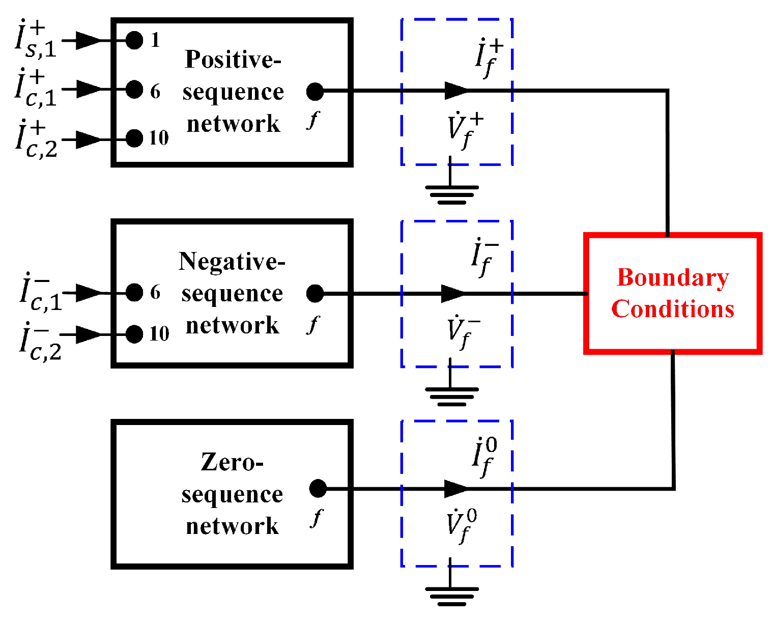
On the other hand, the faulted network is defined by the boundary conditions which are based on the fault type. The boundary conditions are the same as for the conventional method, where a two-phase fault means parallel-connecting positive- and negative-sequence networks, a single-phase-to-ground fault means that all three sequence networks are series-connected, while a two-phase-to-ground fault means all three-sequence networks are parallel-connected. From the calculations in Equations (13) and (14), the sequence voltages as seen from the faulted bus f in the normal network can be identified as ${\dot{V}}_f^{+}\left(m\right)$ and ${\dot{V}}_f^{-}\left(m\right)$. Given the bus impedance matrices ${\mathbf{Z}}^{+}$, ${\mathbf{Z}}^{-}$ and ${\mathbf{Z}}^0$, the self-impedances of the bus f in each sequence network can be identified as $Z_{ff}^{+}$, $Z_{ff}^{-}$ and $Z_{ff}^0$. Therefore, the boundary conditions for different types of faults can be illustrated by the circuits in Figure 1, where $Z_f$ represents the fault impedance.

For a single-phase-to-ground fault, the fault current after the m-th iteration can be obtained based on Figure 1a:

$$\begin{array}{c}\hfill {\dot{I}}_f^{+}\left(m\right)={\dot{I}}_f^{-}\left(m\right)={\dot{I}}_f^0\left(m\right)=\frac{{\dot{V}}_f^{+}\left(m\right)+{\dot{V}}_f^{-}\left(m\right)}{Z_{ff}^{+}+Z_{ff}^{-}+Z_{ff}^0+3Z_f}.\end{array}$$

(16)

For a two-phase fault, the fault current after the m-th iteration can be obtained based on Figure 1b:

$$\begin{array}{c}\hfill {\dot{I}}_f^{+}\left(m\right)=-{\dot{I}}_f^{-}\left(m\right)=\frac{{\dot{V}}_f^{+}\left(m\right)-{\dot{V}}_f^{-}\left(m\right)}{Z_{ff}^{+}+Z_{ff}^{-}+Z_f}.\end{array}$$

(17)

For a two-phase-to-ground fault, the fault current after the m-th iteration can be obtained based on Figure 1c:

$$\begin{array}{cc}\hfill {\dot{I}}_f^{+}\left(m\right)& =\frac{{\dot{V}}_f^{+}\left(m\right)-{\dot{V}}_f^{-}\left(m\right)+\frac{Z_{ff}^{-}{\dot{V}}_f^{-}\left(m\right)}{Z_{ff}^{-}+Z_{ff}^0+3Z_f}}{Z_{ff}^{+}+\frac{Z_{ff}^{-}(Z_{ff}^0+3Z_f)}{Z_{ff}^{-}+Z_{ff}^0+3Z_f}}\hfill \end{array}$$

(18)

$$\begin{array}{cc}\hfill {\dot{I}}_f^{-}\left(m\right)& =\frac{{\dot{V}}_f^{-}\left(m\right)-{\dot{V}}_f^{+}\left(m\right)+Z_{ff}^{+}{\dot{I}}_f^{+}}{Z_{ff}^{-}}\hfill \end{array}$$

(19)

$$\begin{array}{cc}\hfill {\dot{I}}_f^0\left(m\right)& =-{\dot{I}}_f^{+}\left(m\right)-{\dot{I}}_f^{-}\left(m\right).\hfill \end{array}$$

(20)

Then, the voltage drops on all buses caused by the fault in each sequence network can be calculated by

$$\begin{array}{cc}\hfill \Delta {\mathbf{V}}^{+}\left(m\right)& ={\left[Z_{1f}^{+},Z_{2f}^{+},\dots ,Z_{Nf}^{+}\right]}^T·{\dot{I}}_f^{+}\left(m\right)\hfill \end{array}$$

(21)

$$\begin{array}{cc}\hfill \Delta {\mathbf{V}}^{-}\left(m\right)& ={\left[Z_{1f}^{-},Z_{2f}^{-},\dots ,Z_{Nf}^{-}\right]}^T·{\dot{I}}_f^{-}\left(m\right)\hfill \end{array}$$

(22)

$$\begin{array}{cc}\hfill \Delta {\mathbf{V}}^0\left(m\right)& ={\left[Z_{1f}^0,Z_{2f}^0,\dots ,Z_{Nf}^0\right]}^T·{\dot{I}}_f^0\left(m\right).\hfill \end{array}$$

(23)

Finally, the sequence voltages after the m-th iteration on all buses are updated using the superposition:

$$\begin{array}{cc}\hfill {\mathbf{V}}^{+}\left(m\right)& ={\mathbf{V}}^{+}\left(m\right)-\Delta {\mathbf{V}}^{+}\left(m\right)\hfill \end{array}$$

(24)

$$\begin{array}{cc}\hfill {\mathbf{V}}^{-}\left(m\right)& ={\mathbf{V}}^{-}\left(m\right)-\Delta {\mathbf{V}}^{-}\left(m\right)\hfill \end{array}$$

(25)

$$\begin{array}{cc}\hfill {\mathbf{V}}^0\left(m\right)& =-\Delta {\mathbf{V}}^0\left(m\right)\hfill \end{array}$$

(26)

For the next iteration, the sequence voltages of all converter terminals obtained by Equations (24)–(26) are substituted into Equations (9) and (10) to update the current references. The whole procedure from Equation (9) to Equation (26) is repeated until the current references of all converters reach convergence. Figure 2 presents the flow chart of the proposed fault analysis method.

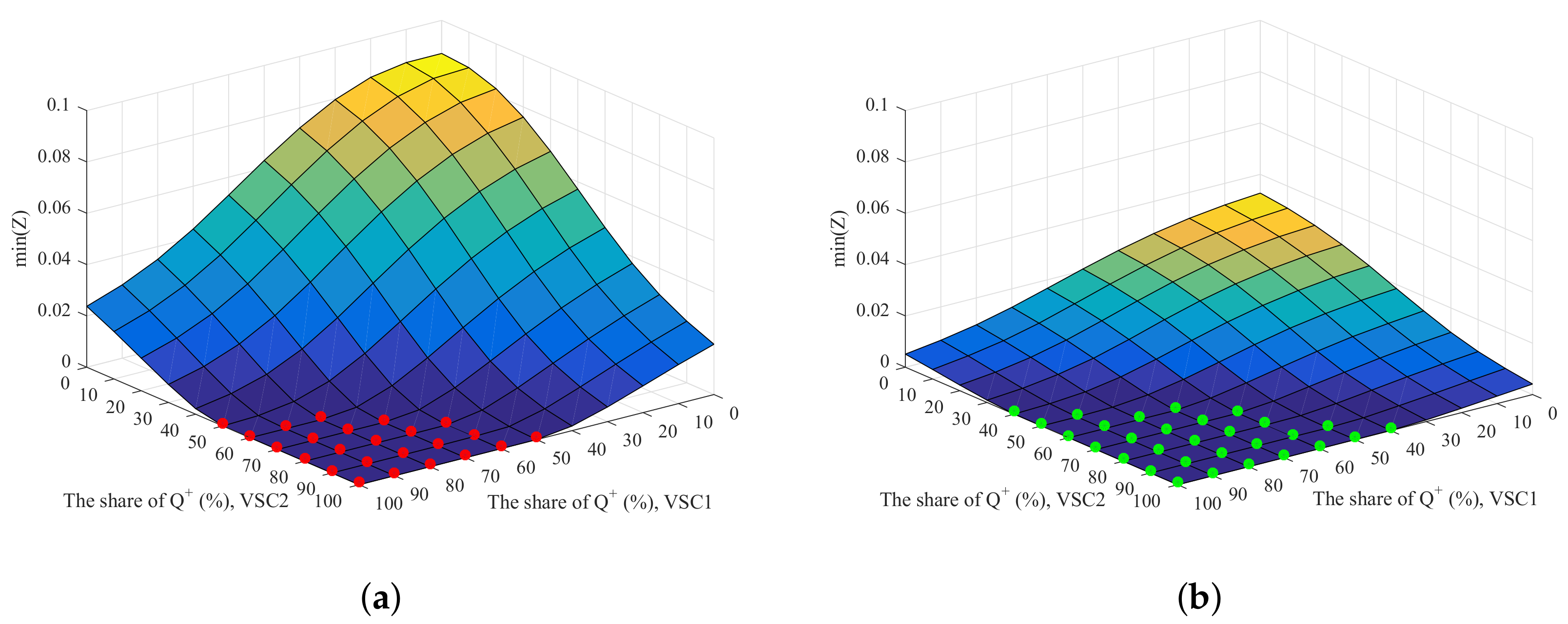
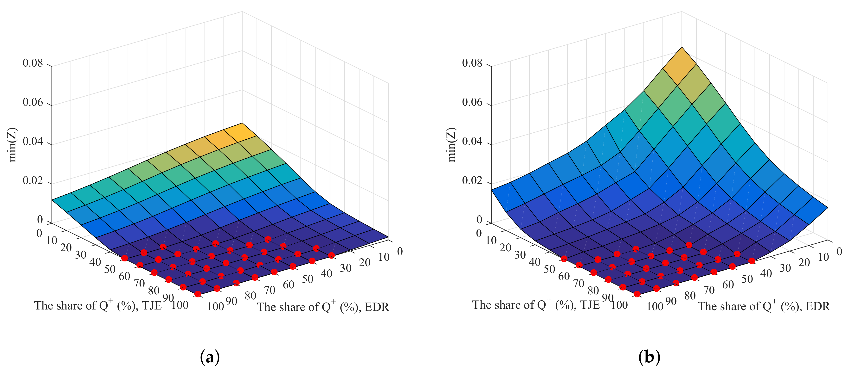
2.3. Verification

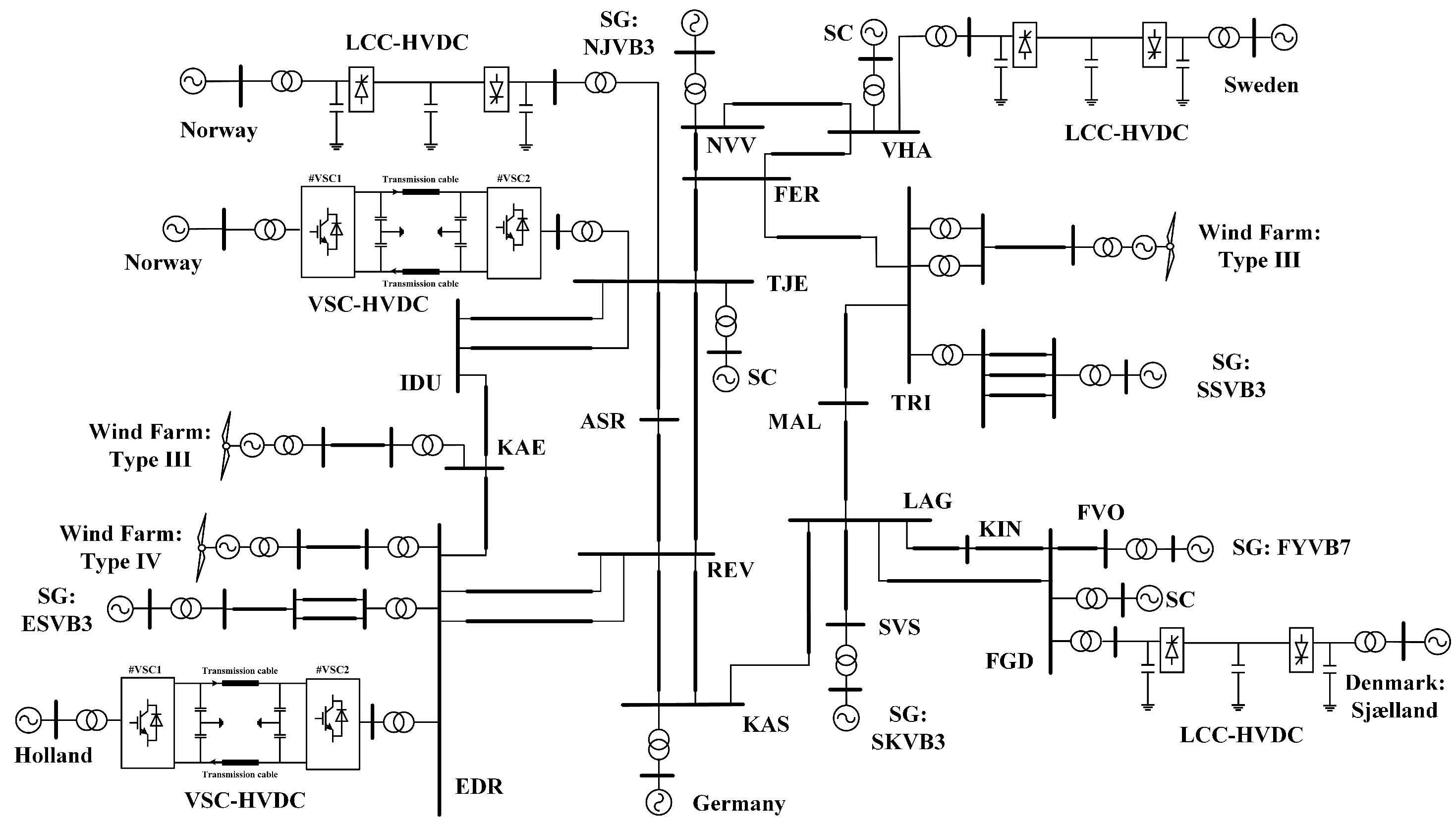
The proposed fault analysis method was firstly tested on a modified IEEE 9-bus system, as shown in Figure 3. The modifications to the original system [32] were (1) the system voltage level was increased to 400 kV; (2) the synchronous generators connected to bus 6 and bus 10 were replaced by VSC1 and VSC2, respectively. The current references of both converters under grid unbalanced faults were in the form of Equations (3) and (4); (3) one more bus (bus 2) was added compared to the original system; (4) the parameters of all transmission lines, transformers and machines were replaced by real data. Figure 4 illustrates the sequence networks when there is a fault at bus f. In the positive-sequence network, there were three current injections, ${\dot{I}}_{s,1}^{+}$ (from SG), ${\dot{I}}_{c,1}^{+}$ and ${\dot{I}}_{c,2}^{+}$ (from VSC1 and VSC2), while in the negative-sequence network there were two current injections ${\dot{I}}_{c,1}^{-}$ and ${\dot{I}}_{c,2}^{-}$ (from VSC1 and VSC2). Therefore, Equations (11) and (12) became

$$\begin{array}{cc}\hfill {\mathbf{I}}_{inj}^{+}\left(m\right)& ={\left[{\dot{I}}_{s,1}^{+},0,0,0,0,{\dot{I}}_{c,1}^{+}\left(m\right),0,0,0,{\dot{I}}_{c,2}^{+}\left(m\right)\right]}^T\hfill \end{array}$$

(27)

$$\begin{array}{cc}\hfill {\mathbf{I}}_{inj}^{-}\left(m\right)& ={\left[0,0,0,0,0,{\dot{I}}_{c,1}^{-}\left(m\right),0,0,0,{\dot{I}}_{c,2}^{-}\left(m\right)\right]}^T.\hfill \end{array}$$

(28)

Prior to the fault, VSC1 and VSC2 were delivering 165 MW and 75 MW active power, respectively, at the unity power factor. The voltage on bus 1 was maintained at 1 p.u. It was assumed that under fault conditions there were $P_{ref}=165$ MW, $Q_{ref}=50$ Mvar for VSC1 and $P_{ref}=75$ MW, $Q_{ref}=250$ Mvar for VSC2. For VSC2, the control strategy was characterized by $a_2=c_2=1$ (providing only positive-sequence short circuit powers $P^{+}$ and $Q^{+}$). For VSC1, the control strategy (characterized by $a_1$ and $c_1$) was varied under different scenarios which are summarized in

Table 1. Different scenarios of voltage source converter (VSC)1 control strategies.

Scenario	${\mathit{a}}_1$	${\mathit{c}}_1$	Share of Sequence Powers
S1	1	1	$P^{+}$(100%), $P^{-}$(0%), $Q^{+}$(100%), $Q^{-}$(0%)
S2	1	0.5	$P^{+}$(100%), $P^{-}$(0%), $Q^{+}$(50%), $Q^{-}$(50%)
S3	1	0	$P^{+}$(100%), $P^{-}$(0%), $Q^{+}$(0%), $Q^{-}$(100%)
S4	0.5	1	$P^{+}$(50%), $P^{-}$(50%), $Q^{+}$(100%), $Q^{-}$(0%)

. For the purpose of verifying the calculated results, the system shown in Figure 3 was also modeled in a RTDS. The dual-sequence current control block diagram of the VSCs under fault conditions is illustrated by Figure 5, where two current control loops implemented in the synchronous refernece frame were used to track the positive- and negative-sequence current references. 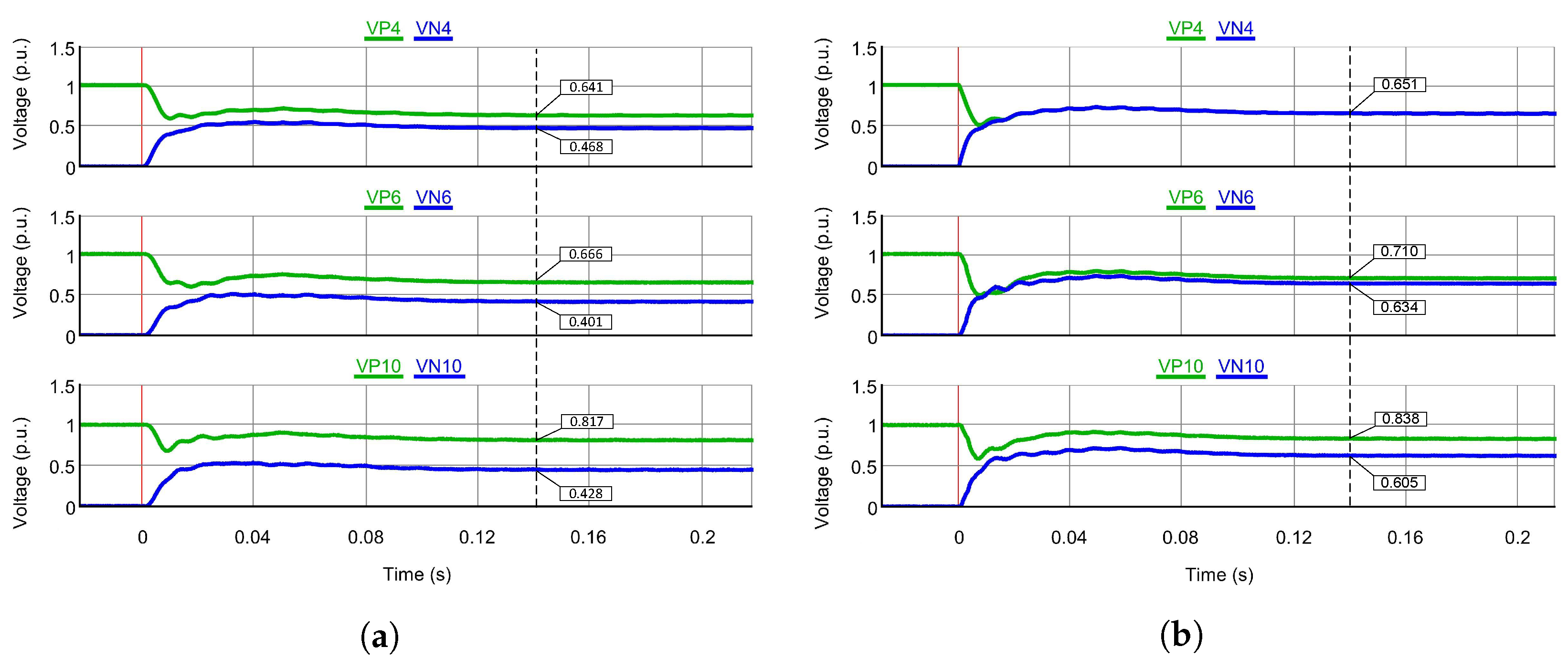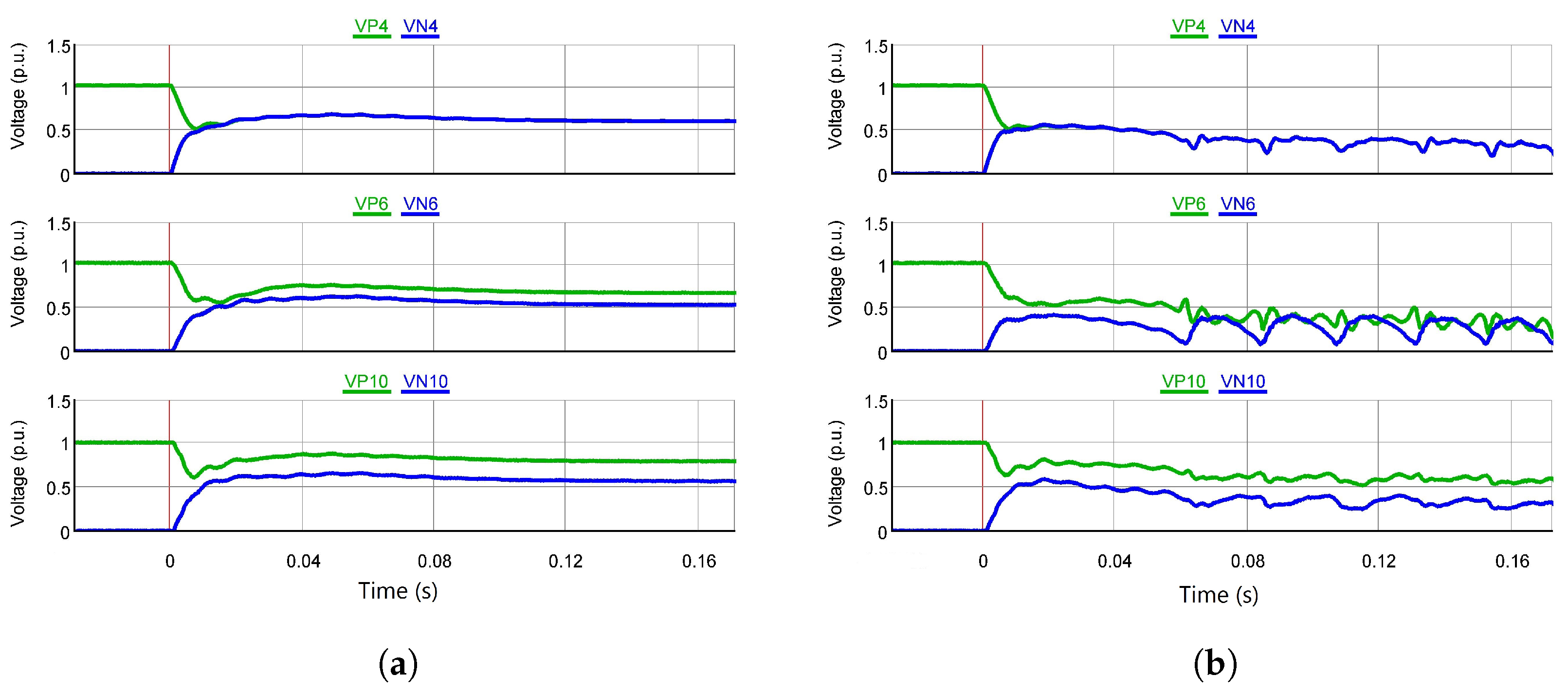The angle $\theta$ used by the Park transformation was obtained by the Dual Second Order Generalized Integrator Phase Locked Loop (DSOGI-PLL) presented in [33]. The results calculated from the proposed fault analysis method were compared with the RTDS simulations for verification. For example, with a solid A–B fault or A–g fault on bus 4, Figure 6 presents the RTDS simulations of the sequence voltages of the faulted bus (bus 4) and the PCC points (bus 6 and 10) in two scenarios: A–g fault with S3 and A–B fault with S4. For these two scenarios, Figure 7 presents the simulated short circuit currents from the VSCs. As a summary for the different scenarios,

Table 2. Comparison between calculations and simulations (S1).

	A–B Fault				A–g Fault
Bus	$\left|{\dot{V}}^{+}\right|$ (p.u.)		$\left|{\dot{V}}^{-}\right|$ (p.u.)		$\left|{\dot{V}}^{+}\right|$ (p.u.)		$\left|{\dot{V}}^{-}\right|$ (p.u.)
	Cal	RTDS	Cal	RTDS	Cal	RTDS	Cal	RTDS
4	0.636	0.645	0.636	0.645	0.721	0.726	0.551	0.558
6	0.692	0.699	0.619	0.625	0.773	0.780	0.536	0.542
10	0.817	0.821	0.591	0.599	0.886	0.893	0.512	0.520
Converter	$\left|{\dot{I}}^{+}\right|$ (p.u.)		$\left|{\dot{I}}^{-}\right|$ (p.u.)		$\left|{\dot{I}}^{+}\right|$ (p.u.)		$\left|{\dot{I}}^{-}\right|$ (p.u.)
1	0.263	0.260	0	0	0.223	0.228	0	0
2	0.320	0.317	0	0	0.279	0.282	0	0

,

Table 3. Comparison between calculations and simulations (S2).

	A–B Fault				A–g Fault
Bus	$\left|{\dot{V}}^{+}\right|$ (p.u.)		$\left|{\dot{V}}^{-}\right|$ (p.u.)		$\left|{\dot{V}}^{+}\right|$ (p.u.)		$\left|{\dot{V}}^{-}\right|$ (p.u.)
	Cal	RTDS	Cal	RTDS	Cal	RTDS	Cal	RTDS
4	0.599	0.605	0.599	0.605	0.684	0.690	0.513	0.519
6	0.640	0.646	0.564	0.570	0.723	0.727	0.477	0.485
10	0.785	0.792	0.554	0.563	0.854	0.859	0.473	0.480
Converter	$\left|{\dot{I}}^{+}\right|$ (p.u.)		$\left|{\dot{I}}^{-}\right|$ (p.u.)		$\left|{\dot{I}}^{+}\right|$ (p.u.)		$\left|{\dot{I}}^{-}\right|$ (p.u.)
1	0.276	0.271	0.044	0.041	0.235	0.238	0.050	0.058
2	0.332	0.034	0	0	0.298	0.297	0	0

,

Table 4. Comparison between calculations and simulations (S3).

	A–B Fault				A–g Fault
Bus	$\left|{\dot{V}}^{+}\right|$ (p.u.)		$\left|{\dot{V}}^{-}\right|$ (p.u.)		$\left|{\dot{V}}^{+}\right|$ (p.u.)		$\left|{\dot{V}}^{-}\right|$ (p.u.)
	Cal	RTDS	Cal	RTDS	Cal	RTDS	Cal	RTDS
4	0.549	0.556	0.549	0.556	0.634	0.641	0.460	0.468
6	0.571	0.580	0.491	0.499	0.658	0.666	0.394	0.401
10	0.742	0.750	0.504	0.510	0.812	0.817	0.420	0.428
Converter	$\left|{\dot{I}}^{+}\right|$ (p.u.)		$\left|{\dot{I}}^{-}\right|$ (p.u.)		$\left|{\dot{I}}^{+}\right|$ (p.u.)		$\left|{\dot{I}}^{-}\right|$ (p.u.)
1	0.306	0.301	0.102	0.096	0.269	0.264	0.114	0. 115
2	0.351	0.350	0	0	0.328	0.326	0	0

and

Table 5. Comparison between calculations and simulations (S4).

	A–B Fault				A–g Fault
Bus	$\left|{\dot{V}}^{+}\right|$ (p.u.)		$\left|{\dot{V}}^{-}\right|$ (p.u.)		$\left|{\dot{V}}^{+}\right|$ (p.u.)		$\left|{\dot{V}}^{-}\right|$ (p.u.)
	Cal	RTDS	Cal	RTDS	Cal	RTDS	Cal	RTDS
4	0.645	0.651	0.645	0.651	0.725	0.732	0.558	0.564
6	0.704	0.710	0.626	0.634	0.779	0.787	0.541	0.546
10	0.834	0.838	0.599	0.605	0.890	0.899	0.518	0.525
Converter	$\left|{\dot{I}}^{+}\right|$ (p.u.)		$\left|{\dot{I}}^{-}\right|$ (p.u.)		$\left|{\dot{I}}^{+}\right|$ (p.u.)		$\left|{\dot{I}}^{-}\right|$ (p.u.)
1	0.143	0.142	0.140	0.138	0.123	0.124	0.152	0.149
2	0.317	0.312	0	0	0.278	0.282	0	0

compare the RMS values of the sequence voltages as well as the RMS values of the sequence currents contributed by the VSCs during the fault. It can be observed that the results obtained from the proposed method agree with the simulations. This verifies that the proposed method is able to perform static fault analysis considering the dual-sequence current control of VSCs. Errors could arise from the fact that the short-circuit impedance of a synchronous generator is a time-varying quantity, and RTDS performs the simualtions in real time. The power system in RTDS was modeled with details for all the components. During the fault, the system’s dynamics cannot be completely reflected by the static fault analysis.

By comparing the results from S1 with S4, it can be seen that changes in sequence active powers ($P^{+}$, $P^{-}$) do not alter the retained grid voltages notably. However, when comparing S1, S2 and S3, it can be observed that changes in sequence reactive powers ($Q^{+}$, $Q^{-}$) have more effects on the retained voltages. This is reasonable since the voltages of an inductive grid are mainly regulated by reactive power. Different control strategies could yield different values for factor c, hence changing the combination of $Q^{+}$ and $Q^{-}$.

3. The Impact of Dual-Sequence Current Control on the System

3.1. Problem Description

Regarding the test system used in Section 2.3, it was observed from the RTDS simulations that, with different combinations of $Q^{ref}$ and $c_1$, not all scenarios gave a stable response under fault conditions. As an example, when all other parameters remained the same, the reactive power reference of VSC1 under fault conditions increased to 150 Mvar (50 Mvar previously). Then, the scenarios S2 and S3, defined in Table 1, were simulated again in RTDS. Figure 8a presents the simulation results of the sequence voltages on bus 4, bus 6 and bus 10 for S2, which correspond to a solid A–B fault on bus 4 at the zero time instant. After the fault is initiated, both positive- and negative-sequence voltages were able to retain at a certain level and exhibited stable responses. However, as shown in Figure 8b for S3, both sequence voltages did not stabilize at a certain level but exhibited oscillatory behaviours. Regarding this unstable scenario, the proposed fault analysis method was applied to check the obtained results. Correspondingly, the algorithm was not able to reach a convergence even after a large number of iterations. Therefore, an initial guess of the explanation for Figure 8b is that the system does not have a solution so that a stable operating point cannot be found by RTDS.

3.2. Problem Formulation Using the Proposed Fault Analysis Method

In order to investigate and explain the phenomenon in Figure 8b, an optimization approach was used to explore the solution to the system with the application of the proposed fault analysis method. In addition, the reactive power references were generated using pre-assumed grid codes rather than fixed values. The objective function was defined as:

$$\begin{array}{c}\hfill \begin{array}{cc}\hfill minZ& =\sum _j\left\{{[Q_{c,j}^{ref}-F_Q\left({\dot{V}}_{c,j}^{+}\right)]}^2\right\}\hfill \\ & +\sum _j\left\{{\left\{\Re \left({\dot{I}}_{c,j}^{+}\right)-\Re \left[F^{+}\left({\dot{V}}_{c,j}^{+}\right)\right]\right\}}^2\right\}+\sum _j\left\{{\left\{\Re \left({\dot{I}}_{c,j}^{-}\right)-\Re \left[F^{+}\left({\dot{V}}_{c,j}^{-}\right)\right]\right\}}^2\right\}\hfill \\ & +\sum _j\left\{{\left\{\Im \left({\dot{I}}_{c,j}^{+}\right)-\Im \left[F^{+}\left({\dot{V}}_{c,j}^{+}\right)\right]\right\}}^2\right\}+\sum _j\left\{{\left\{\Im \left({\dot{I}}_{c,j}^{-}\right)-\Im \left[F^{+}\left({\dot{V}}_{c,j}^{-}\right)\right]\right\}}^2\right\}\hfill \end{array}\end{array}$$

(29)

where the reactive power reference for the j-th conveter $Q_{c,j}^{ref}$, the real part $\Re ({\dot{I}}_{c,j}^{+})$, $\Re ({\dot{I}}_{c,j}^{-})$ and the imaginary part $\Im ({\dot{I}}_{c,j}^{+})$, $\Im ({\dot{I}}_{c,j}^{-})$ of the current references are considered to be the optimization variables; $F^{+}$ and $F^{-}$ refer to the current references using Equations (9) and (10), respectively; while ${\dot{V}}_{c,j}^{+}$ and ${\dot{V}}_{c,j}^{-}$ are obtained using Equations (11)–(26). Generally, grid codes regarding reactive power support are defined in the form of a profile of the reactive current requirement versus the voltage at the PCC. Since the power is a product of voltage and current, the reactive power references can be regarded as functions of the PCC voltages. In this paper, the reactive power reference of a VSC under grid unbalanced faults was considered to be a function ($F_Q$) of the positive-sequence voltage at the PCC. Per unit values were used for all the above quantities during the optimization. Ideally, if a solution to the system exists, the substitution of the solution into Equation (29), should yield a value of zero for Z. Therefore, the value of $min\left(Z\right)$ could be used as an indication of whether a solution to the system exists.

3.3. Investigation and Discussion

For the system in Figure 3, the pre-fault conditions were kept the same as those in Section 2.3. The reactive power reference was assumed to be generated using the function $F_Q\left({\dot{V}}_{c,j}^{+}\right)=\left|{\dot{V}}_{c,j}^{+}\right|·I_{Q,j}$, where the value of $I_{Q,j}$ was obtained according to the profiles in Figure 9. Here, two different profiles were considered. Profile 1 is expressed mathmatically by $I_{Q,j}=-2.5\left|{\dot{V}}_{c,j}^{+}\right|+2.25(0\le I_{Q,j}\le 1)$, which is obtained from [34]. Profile 2 is expressed by $I_{Q,j}=-1.25\left|{\dot{V}}_{c,j}^{+}\right|+1.25(0\le I_{Q,j}\le 0.5)$. In this paper, profile 2 is used to represent a case where VSCs feed less reactive power to the grid compared to profile 1. In this investigation, the control strategy factors $a_1$ and $a_2$ were fixed at 1, meaning both converters did not provide $P^{-}$. However, the control strategy factors $c_1$ and $c_2$ for VSC1 and VSC2 were varied between 0 and 1 with a step of 0.1 to show different scenarios. This means that the share of the $Q^{+}$ contributed by each VSC varied from 0% to 100% with a 10% step. The optimization problem, defined in Section 3.2, was a nonlinear programming (NLP) problem with (29) as the objective function. The proposed fault analysis method, (7)–(26), as well as the grid codes served as the contraints. In this paper, the optimization was perfomed with the MATLAB optimization toolbox [35] using the genetic algorithm. For a two-phase fault at bus 4, the optimization procedure was repeated with all possible combinations of $c_1$ and $c_2$.

Figure 10 shows the values of $min\left(Z\right)$ under different scenarios after the optimization. Figure 10a is the case when profile 1 was used to generate the reactive power references, while Figure 10b is the case when profile 2 was used. For both cases, the scenario marked by a dot has an objective function value below ${10}^{-4}$. Correspondingly, the simulation results from RTDS gave stable responses, like in Figure 8a during the fault. However, for the rest of the scenarios without a dot, the values of $min\left(Z\right)$ were all above ${10}^{-4}$, and RTDS showed an oscillatory behaviour, like in Figure 8b. The less the share of $Q^{+}$ was, the further $min\left(Z\right)$ was away from zero. This indicates that the injection of $Q^{-}$ may result in situations where the system cannot find an stable operating point to satisfy Equations (7)–(26) and the reactive power requirement at the same time.

As illustrated in Figure 4, when the VSCs are able to provide negative-sequence current, the negative-sequence network under fault conditions becomes active. This is significantly different from that of a conventional system whose negative-sequence network is passive. For an inductive grid, the injection of $Q^{+}$ and $Q^{-}$ could alter the PCC voltages in both positive- and negative-sequence networks; these changes will in turn affect the current references of VSCs in both the positive- and negative-sequence networks. Together with the boundary conditions linking the different sequence networks that are defined by the fault type, then the system may not have a solution to fulfil all these restrictions. On the other hand, the surface in Figure 10b is closer to zero than that of Figure 10a and a more stable scenario exists in Figure 10b. This is because, with profile 2, less reactive power is injected, and hence, the injection of $Q^{-}$ does not impact the system as much as that with profile 1. Therefore, the system can tolerate a higher share of $Q^{-}$ (with more stable scenarios) than that with profile 1.

4. Application on the Western Danish Power System

In this section, the proposed fault analysis method is applied to a larger system (shown in Figure 11) for further verification. This is a simplified version of the Western Danish power system (DK1) for a 2020 scenario with new planned transmission lines and a new VSC–HVDC link to Holland. Each 400 kV bus is assigned a three-letter name. In this system, there are two VSC-HVDC links at TJE and EDR. to the neighbouring countries and one Type-IV to a wind farm near EDR. These three VSC-based sources are assumed to have the dual-sequence current control in the form of Equations (3) and (4). Three synchronous condensers (SCs) are connected to the grid at VHA, TJE and FGD. Since an SC is principally an SG without the prime mover, the short-circuit model using Equations (7) and (8) for SGs also applies to the SCs. Two Type-III wind farms are integrated into the system near KAE and TRI, and they are treated as conventional induction motors for the fault analysis [21]. The parameters of all synchronous machines, transformers and transmission lines are provided by the Danish TSO Energinet.dk. The whole system was also modeled in RTDS for verification.

Firstly, the calculation results using the proposed fault analysis method in Section 2 were compared with those obtained from the simulations. As an example, with the control strategy factors a and c set to 1 (providing only $P^{+}$ and $Q^{+}$) for all the three VSC-based sources,

Table 6. Comparison between calculations and simulations (A–B fault).

	$\left|{\dot{\mathit{V}}}^{+}\right|$ (p.u.)						$\left|{\dot{\mathit{V}}}^{-}\right|$ (p.u.)
Bus	IDU	EDR	TJE	FER	TRI	LAG	IDU	EDR	TJE	FER	TRI	LAG
Cal	0.524	0.664	0.627	0.689	0.736	0.765	0.524	0.374	0.424	0.338	0.288	0.274
RTDS	0.518	0.658	0.622	0.681	0.730	0.758	0.518	0.368	0.416	0.329	0.279	0.265

and

Table 7. Comparison between calculations and simulations (A–g fault).

	$\left|{\dot{\mathit{V}}}^{+}\right|$ (p.u.)						$\left|{\dot{\mathit{V}}}^{-}\right|$ (p.u.)
Bus	IDU	EDR	TJE	FER	TRI	LAG	IDU	EDR	TJE	FER	TRI	LAG
Cal	0.630	0.738	0.706	0.747	0.786	0.817	0.354	0.278	0.280	0.220	0.184	0.168
RTDS	0.624	0.731	0.701	0.738	0.778	0.810	0.346	0.267	0.272	0.211	0.196	0.175

compare the retained sequence voltages of certain buses subject to a solid A–B or A–g fault at IDU. It can be observed that the calculation results agree with the RTDS simulation results.

Secondly, the investigation performed in Section 3 was applied to the DK1 system. For the Type-IV wind farm, it was assumed that there was $a=c=1$ (providing only $P^{+}$ and $Q^{+}$). For the two VSC-HVDC stations at EDR and TJE, there was $a=1$ (providing only $P^{+}$). However, their control strategy factor c varied between 0 and 1 with a step of 0.1 for different scenarios. This means that the share of $Q^{+}$ contributed by these two VSC-HVDC stations varied from 0% to 100% with a 10% step. The reactive power references for all these three VSC-based sources were generated using profile 1 in Figure 9. The optimization was performed for all possible combinations of c. For a solid A–B fault at IDU, Figure 12a illustrates the values of $min\left(Z\right)$ under different scenarios. Once again, the scenarios marked by a dot had objective function values below ${10}^{-4}$, and the RTDS simulations gave stable responses, like in Figure 8a, after the fault occurred. For the rest of the scenarios, the values of $min\left(Z\right)$ were all above ${10}^{-4}$ and oscillatory behaviour, like in Figure 8b, was observed in the simulations. For the unstable scenarios, the higher the share of $Q^{-}$ was, the further $min\left(Z\right)$ was away from zero.

As a comparison, the optimization procedure is repeated for the same fault at the same location with three SGs (ESVB3, SKVB3 and NJVB3) disconnected from the grid. Figure 12b presents the values of $min\left(Z\right)$ under different scenarios. Compared to Figure 12a, the surface in Figure 12b was further away from zero and a less stable scenario existed. In this case, with three more synchronous generators phased-out, the system short circuit power was lower. As a result, the reactive power support from VSCs had more impact on the system, and the system tolerated less $Q^{-}$ injections from VSCs. This suggests that the deployment of the dual-sequence current control strategies for future converter-dominated power systems involving negative-sequence reactive current provision should be re-evaluated considering their adverse impact on the systems. The existence of the solution to (7)–(26) can be used as an indicator of whether the system has a stable fault response with consideration of the dual-sequence current control of VSCs. Therefore, the proposed method has the potential to help with defining and evaluating grid codes regarding the requirements of negative-sequence current injection from VSCs.

5. Conclusions

This paper developed a static fault analysis method that considers the dual-sequence current control of VSCs under grid unbalanced faults. In this method, the VSCs are treated as voltage-dependent current sources with flexible parameters that represent different control strategies. The proposed method was verified through simulations in two different systems and can be applied to a system with multiple VSCs. Throughout the RTDS simulations, it was discovered that the negative-sequence current injection from VSCs may result in an unstable fault response of the system. The proposed fault analysis method was used to help explain this phenomenon and showed that the unstable response is due to the fact that the system cannot find a solution. This phenomenon could occur when the share of negative-sequence reactive power from VSCs is high or when the system has a low short circuit power. The proposed method can help engineers to better understand and evaluate the impact of the dual-sequence current control of VSCs on future converter-dominated power systems.

References

1. Yazdani, A.; Iravani, R. Voltage-Sourced Converters in Power Systems: Modeling, Control, and Applications; John Wiley & Sons, Inc.: Hoboken, NJ, USA, 2010. [Google Scholar]
2. Mohseni, M.; Islam, S.M. Review of international grid codes for wind power integration: diversity, technology and a case for global standard. Renew. Sustain. Energy Rev. 2012, 16, 3876–3890. [Google Scholar] [CrossRef]
3. Crăciun, B.I.; Kerekes, T.; Séra, D.; Teodorescu, R. Overview of recent grid codes for PV power integration. In Proceedings of the 13th International Conference on Optimization of Electrical and Electronic Equipment (OPTIM), Brasov, Romania, 24–26 May 2012; pp. 959–965. [Google Scholar]
4. Establishing a Network Code on Requirements for Grid Connection of High Voltage Direct Current Systems and Direct Current-Connected Power Park Modules; ENTSO-E: Brussels, Belgium, 2016.
5. Jia, J.; Yang, G.; Nielsen, A.H. A review on grid-connected converter control for short circuit power provision under grid unbalanced faults. IEEE Trans. Power Deliv. 2018, 33, 649–661. [Google Scholar] [CrossRef]
6. IEC 60909-0 Short-Circuit Currents in Three-Phase a.c. Systems–Calculation of Currents; International Electrotechnical Commission (IEC): Geneva, Switzerland, 2001.
7. Muljadi, E.; Samaan, N.; Gevorgian, V.; Li, J.; Pasupulati, S. Different factors affecting short circuit behavior of a wind power plant. IEEE Trans. Ind. Appl. 2013, 49, 284–292. [Google Scholar] [CrossRef]
8. Alam, M.M.; Leite, H.; Silva, N.; Carvalho, A.D.S. Performance evaluation of distance protection of transmission lines connected with VSC-HVDC system using closed-loop test in RTDS. Electr. Power Syst. Res. 2017, 152, 168–183. [Google Scholar] [CrossRef]
9. Wang, F.; Duarte, J.L.; Hendrix, M.A.M. Pliant active and reactive power control for grid-interactive converters under unbalanced voltage dips. IEEE Trans. Power Electron. 2011, 26, 1511–1521. [Google Scholar] [CrossRef]
10. Chen, H.C.; Lee, C.T.; Cheng, P.T.; Teodorescu, P.; Blaabjerg, F. A low-voltage ride-through technique for grid-connected converters with reduced power transistors stress. IEEE Trans. Power Electron. 2016, 31, 8562–8571. [Google Scholar] [CrossRef]
11. Camacho, A.; Castilla, M.; Miret, J.; Guzman, R.; Borrell, A. Reactive power control for distributed generation power plants to comply with voltage limits during grid faults. IEEE Trans. Power Electron. 2014, 29, 6224–6234. [Google Scholar] [CrossRef]
12. Camacho, A.; Castilla, M.; Miret, J.; Vicuña, L.G.D.; Andrés, G.L.M. Control strategy for distribution generation inverters to maximize the voltage support in the lowest phase during voltage sags. IEEE Trans. Ind. Electron. 2018, 65, 2346–2355. [Google Scholar] [CrossRef]
13. Shabestary, M.M.; Mohamed, Y.A.R.I. Analytical expressions for multiobjective optimization of converter-based DG operation under unbalanced grid conditions. IEEE Trans. Power Electron. 2017, 32, 7284–7296. [Google Scholar] [CrossRef]
14. Revelo, S.; Silva, C.A. Current reference strategy with explicit negative sequence component for voltage equalization contribution during asymmetric fault ride through. Int. Trans. Electr. Energy Syst. 2015, 25, 3449–3471. [Google Scholar] [CrossRef]
15. Nejabatkhah, F.; Li, Y.W.; Wu, B. Control strategies of three-phase distributed generation inverters for grid unbalanced voltage compensation. IEEE Trans. Power Electron. 2016, 31, 5228–5241. [Google Scholar]
16. Kabiri, R.; Holmes, D.G.; McGrath, B.P. Control of active and reactive power ripple to mitigate unbalanced grid voltages. IEEE Trans. Ind. Appl. 2016, 52, 1660–1668. [Google Scholar] [CrossRef]
17. Göksu, Ö.; Teodorescu, R.; Bak, C.L.; Iov, F.; Kjaer, P.C. Impact of wind power plant reactive current injection during asymmetrical grid faults. IET Renew. Power Gener. 2013, 7, 484–492. [Google Scholar] [CrossRef]
18. Neumann, T.; Wijnhoven, T.; Deconinck, G.; Erlich, I. Enhanced dynamic voltage control of type 4 wind turbines during unbalanced grid faults. IEEE Trans. Energy Convers. 2015, 30, 1650–1659. [Google Scholar] [CrossRef]
19. Wijnhoven, T.; Deconinck, G.; Neumann, T.; Erlich, I. Control aspects of the dynamic negative sequence current injection of type 4 wind turbines. In Proceedings of the IEEE PES General Meeting | Conference & Exposition, National Harbor, MD, USA, 27–31 July 2014; pp. 1–5. [Google Scholar]
20. Kamh, M.Z.; Iravani, R. A unified three-phase power-flow analysis model for electronically coupled distributed energy resources. IEEE Trans. Power Deliv. 2011, 26, 899–909. [Google Scholar] [CrossRef]
21. Wind Power Plant Short-Circuit Modeling Guide; Technical Report SAND2012-6664; Sandia National Laboratories: Albuquerque, NM, USA; Livermore, CA, USA, 2012.
22. Bui, D.M. Simplified and automated fault-current calculation for fault protection system of grid-connected low-voltage AC microgrids. Int. J. Emerg. Electr. Power Syst. 2017, 18, 1–24. [Google Scholar] [CrossRef]
23. Dağ, B.; Boynueğri, A.R.; Ateş, Y.; Karakaş, A.; Nadar, A.; Uzunoğlu, M. Static modeling of microgrids for load flow and fault analysis. IEEE Trans. Power Syst. 2017, 32, 1990–2000. [Google Scholar] [CrossRef]
24. Plet, C.A.; Green, T.C. Fault response of inverter interfaced distributed generators in grid-connected applications. Electr. Power Syst. Res. 2014, 106, 21–28. [Google Scholar] [CrossRef]
25. Mathur, A.; Das, B.; Pant, V. Fault analysis of unbalanced radial and meshed distribution system with inverter based distributed generation (IBDG). Int. J. Electr. Power Energy Syst. 2017, 85, 164–177. [Google Scholar] [CrossRef]
26. Tu, D.V.; Chaitusaney, S.; Yokoyama, A. Maximum-allowable distributed generation considering fault ride-through requirement and reach reduction of utility relay. IEEE Trans. Power Deliv. 2014, 29, 534–541. [Google Scholar]
27. Moura, A.P.; Lopes, J.P.; Moura, A.A.D.; Sumaili, J.; Moreira, C. IMICV fault analysis method with multiple PV grid-connected inverters for distribution systems. Electr. Power Syst. Res. 2015, 119, 119–125. [Google Scholar] [CrossRef]
28. Hooshyar, H.; Baran, M.E. Fault analysis on distribution feeders with high penetration of PV systems. IEEE Trans. Power Syst. 2013, 28, 2890–2896. [Google Scholar] [CrossRef]
29. Akagi, H.; Watanabe, E.H.; Aredes, M. Instantaneous Power Theory and Applications to Power Conditioning; John Wiley & Sons, Inc.: Hoboken, NJ, USA, 2016. [Google Scholar]
30. Teodorescu, R.; Liserre, M.; Rodríguez, P. Grid Converters for Photovoltaic and Wind Power Systems; John Wiley & Sons, Inc.: Chichester, UK, 2011. [Google Scholar]
31. Kamh, M.Z.; Iravani, R. Unbalanced model and power-flow analysis of microgrids and active distribution systems. IEEE Trans. Power Deliv. 2010, 25, 2851–2858. [Google Scholar] [CrossRef]
32. Anderson, P.M.; Fouad, A.A. Power System Control and Stability, 2nd ed.; John Wiley & Sons, Inc.: Hoboken, NJ, USA, 2011. [Google Scholar]
33. Rodríguez, P.; Teodorescu, R.; Candela, I.; Timbus, A.V.; Liserre, M.; Blaabjerg, F. New positive-sequence voltage detector for grid synchronization of power converters under faulty grid conditions. In Proceedings of the 37th IEEE Power Electronics Specialists Conference, Jeju, Korea, 18–22 June 2006; pp. 1–7. [Google Scholar]
34. Technical Regulation 3.2.5 for Wind Power Plants with a Power Output above 11 kW; Energinet: Fredericia, Denmark, 2015.
35. MathWorks Global Optimization Toolbox Functions. 2015. Available online: https://www.mathworks.com/help/gads/ga.html (accessed on 18 May 2018).
Figure 1. Boundary conditions for faulted networks: (a) single-phase-to-ground fault; (b) two-phase fault; (c) two-phase-to-ground fault.
Energies 11 01660 g001
Figure 2. Flowchart of the proposed fault analysis method.
Energies 11 01660 g002
Figure 3. Single-line diagram of the test system.
Energies 11 01660 g003
Figure 4. Sequence networks of the test system subject to a fault at bus f.
Energies 11 01660 g004
Figure 5. Dual-sequence current control block diagram of the VSC in Real Time Digital Simulator (RTDS).
Energies 11 01660 g005
Figure 6. Sequence voltages from the RTDS simulation of a fault at bus 4: (a) S3, A–g fault. (b) S4, A–B fault. (VP: positive-sequence voltage; VN: negative-sequence voltage; the number refers to the bus number).
Energies 11 01660 g006
Figure 7. VSC short circuit current (measured from the delta winding side) from the RTDS simulation of a fault at bus 4. (IP: positive-sequence current; IN: negative-sequence current).
Energies 11 01660 g007
Figure 8. Sequence voltages from RTDS simulations subject to an A–B fault at bus 4: (a) a stable scenario. (b) an unstable scenario. (VP: positive-sequence voltage; VN: negative-sequence voltage; the number refers to the bus number).
Energies 11 01660 g008
Figure 9. Reactive current profiles used to generate reactive power references.
Energies 11 01660 g009
Figure 10. The values of min(Z) under different scenarios for an A–B fault at bus 4: (a) with profile 1 of Figure 9. (b) with profile 2 of Figure 9.
Energies 11 01660 g010
Figure 11. Single-line diagram of the western Danish power system.
Energies 11 01660 g011
Figure 12. The values of min(Z) under different scenarios for an A–B fault at IDU: (a) the original system. (b) with three SGs (ESVB3, SKVB3 and NJVB3) phased out.
Energies 11 01660 g012