Jaya based Optimization Method with High Dispatchable Distributed Generation for Residential Microgrid

Abstract

This paper presents a model for optimal energy management under the time-of-use (ToU) and critical peak price (CPP) market in a microgrid. The microgrid consists of intermittent dispatchable distributed generators, energy storage systems, and multi-home load demands. The optimal energy management problem is a challenging task due to the inherent stochastic behavior of the renewable energy resources. In the past, medium-sized distributed energy resource generation was injected into the main grid with no feasible control mechanism to prevent the waste of power generated by a distributed energy resource which has no control mechanism, especially when the grid power limit is altered. Thus, a Jaya-based optimization method is proposed to shift dispatchable distributed generators within the ToU and CPP scheduling horizon. The proposed model coordinates the power supply of the microgrid components, and trades with the main grid to reduce its fuel costs, production costs, and also maximize the monetary profit from sales revenue. The proposed method is implemented on two microgrid operations: the standalone and grid-connected modes. The simulation results are compared with other optimization methods: enhanced differential evolution (EDE) and strawberry algorithm (SBA). Finally, simulation results show that the Jaya-based optimization method minimizes the fuel cost by up to 38.13%, production cost by up to 93.89%, and yields a monetary benefit of up to 72.78% from sales revenue.

1. Introduction

Currently, nonrenewable energy resources such as fossil fuel, coal, nuclear, and natural gas are insufficient to meet the supply needs. This is due to the long duration of replenishment, and thus leads to the emergence of renewable energy. On the other hand, renewable energy refers to the energy sources that work to reduce carbon emission and can replenish naturally. Examples include biomass resources as well as solar, wind, geothermal, and hydro resources. Among these, the most used resource is solar energy. Integrating all renewable energy sources (RESs) into a single unit is achieved through a distributed system which has independent failure of components rather than the existing bulk power delivery system. This distributed system ensures that each component within the system interacts with one another to achieve a common objective. A distributed system may not be limited only to coordinating the various system components, but involves the distributed energy resources (DERs). DERs refer to electricity-generating resources or controllable loads that are directly linked to a remote distribution system. DERs provide electricity to meet the regular demand and improve renewable technologies, which facilitates the transition to an intelligent grid. The intelligent grid provides automated control and modern communications technologies to the present grid. DERs make use of a small-scale power generation technology known as distributed generation. Distributed generation, on the other hand, refers to energy generation at the point of consumption and it helps in eliminating the cost, interdependencies, complexity, and inefficiencies linked with transmission and distribution. These DERs are integrated, and the generated energy is sustained with the help of an energy storage system (ESS), which can be referred to as a microgrid (MG). MGs powered by an RES, ESS, or diesel generator are often cost-effective for residential consumers. A MG is a small network of electricity with local sources such as DERs, RESs, ESSs, dispatchable loads (DLs) and a distributed generator (DG) that is usually linked to a centralized electric grid and can function independently [1]. Each component of an MG is described briefly: the DLs or fuel generators are sources of electricity that modify their power output supplied to the electrical grid on demand. Furthermore, an ESS uses capacitors to store electric energy when disconnected from the charging circuit and can be used at a later time. The goal of MGs is to minimize the transmission loss and overload on the main grid [2]. A MG can operate as a standalone system when disconnected from the main grid or as a grid-connected system when connected to the main grid through a point of common coupling (PCC) [3]. The grid-connected system can either sell or buy power from the main grid. The power trading with the main grid has long been known to depend on a specified, pre-determined price per kWh. MG generation output exhibits stochastic and intermittent patterns that are addressed using optimal energy management.

MG energy management is challenging because of numerous DGs using an RES that can naturally lack the capability of dispatch. This is due to the inherent stochastic behaviour of the resources, and the inflexibility of the operational controls. The MG energy management problem is well-aimed at minimizing the operational cost of the remote DER and ensures the power exchange with the main grid. The MG management problem has optimal scheduling characteristics that are useful for the MG master controller (MMC). These scheduling characteristics estimate the instantaneous DLs’ operations in the MG. The MMC ascertains the dispatch of the DER, and provides energy exchange between the main grid and MG through a PCC. The MMC reduces the overall operating cost with various environmental, reliability, technical, and operational constraints [2].

The MG supports the main grid by consistently distributing its own portion of the generated power. However, the changing state of the MG from grid-connected mode to standalone mode can be associated with high generation [1]. High generations can occur at different intervals for which energy exchange between the main grid can be established. Thus, MG power level may drop to zero during standalone operation. In this situation, the MG generation drops or rises instantly because of the load demand and generation instability.

Several pricing schemes are now used to enhance optimal scheduling of dispatchable DGs within the MG scheduling horizon. The balance between the consumption and production of power systems is achieved through different pricing schemes. This gives the utility the opportunity to invest in power, and to provide better management of power resources to meet the exponentially increasing demand. The electricity pricing methods are frequently used in the literature and in practical scenarios for the utility companies. These methods play a vital role, especially in the demand response implementation. An event-based electricity pricing strategy employed for commercial and industrial consumers with the aim of reducing peak loads is known as the CPP [4]. In this strategy, a higher electricity rate is charged during the event and peaks, and it is mostly targeted during the summer and winter seasons. The CPP influences a higher electricity rate during the hour that falls into critical pricing events announced by the utility and reduces during other hours of the year. The time-of-use (ToU) pricing scheme is time-dependent, divides the pricing rate into time slots, and provides the schedule rate for each time slot [5]. The price is higher during on-peak hours and lower during the off-peak hours. In some cases, ToU schemes make use of mid-peak time slots which fall within the on-peak or off-peak hours. The ToU is more efficiently, simpler, and fairer than the flat rate pricing scheme because it enables load shifting from on-peak to off-peak hours. This scheme is easy for consumers to predict and comprehend, and it encourages the adoption of RESs and distributed storage systems by providing a reduced rate during the on-peak hours. Overall, ToU is proven not to support large peak reduction, and its changing nature allows the price signal to be averaged over an immense period of peak hours or averaged over a minimal number of intense priced hours. In this paper, we consider the hourly CPP and ToU market prices obtained from the utility.

Presently, the standalone operational mode of MGs is faced with the problem of optimal control policies. These policies are useful for determining battery lifespan as well as ESS operation. In this paper, the battery state of charge (SOC) is analyzed based on the charging and discharging operations. DERs can be efficiently scheduled in order to get the optimal operational goals adaptable into the power system. In the past, medium-sized DER generation was injected into the main grid with no feasible control mechanism. Examples include the power generation of wind turbine (WT) and photovoltaic (PV) plants. To prevent the potential waste of power generated by DERs with no control mechanism, especially when the grid limits are violated, these considerations call for optimal energy management implementation. In this paper, we consider an urban residential area with more than one hundred homes, each home using the same appliances and load consumption. This assumption was made in order to make a fair analysis of daily energy demand. Furthermore, this paper proposes an optimal energy scheduling technique to shift dispatchable DGs within the time-based and event-based time price horizon. It also enables the coordination of power supply to satisfy the hourly load demand.

The organization of this paper is as follows. In Section 2 , a related work on the optimal energy management of dispatchable distributed generators in a MG system is given. In Section 3, the optimal energy scheduling problem is formulated with two case studies. Section 4 provides a description of the proposed system model, and the results are presented in Section 5. Finally, Section 6 gives the conclusions of the work and future work.

2. Related Work

The related work in this paper is divided into two components: firstly, we discuss energy management using the deterministic and chance-constrained approaches; and secondly, we discuss energy management using heuristic approaches. Currently, because of the integration of several RESs into MGs, optimizing electric power becomes a necessity—mostly for standalone and grid-connected MGs. Importantly, a high generation of renewable energy that is saddled with uncertainty makes RESs a difficult energy management system (EMS) for MGs. ESSs have been known to increase the efficacy of power supplies by lowering load fluctuations. MG operations involve the scheduling of dispatchable local units of distributed generation and coordinating discharging and charging operations of the storage systems. These MG features maintain DLs with the goal of satisfying the consumer’s load requirement. Currently, the optimal operation of an energy system depends on the ESS, dispatchable DGs, and the electric market tariff.

2.1. Energy Management Using Deterministic and Chance-Constrained Optimization Approaches

In last couple of years, appreciable efforts have been suggested for the energy management of standalone and grid-connected MG operational modes [6,7,8,9,10,11]. Specifically, probabilistic programming models have been proposed in [12,13], while dynamic programming models are suggested in [14,15]. These dynamic and stochastic methods require fine-tuning in their algorithm-specific control parameters. The fine-tuning effect determines the performance of the algorithms in achieving global or local optimum solutions [16]. Optimal energy management in industrial MGs has been considered [17,18,19], whereas residential MG optimal energy management is proposed in [20,21,22,23]. Due to the stochastic nature of RESs, deterministic approaches may not ensure the quality of power which an MG can generate. This problem can be due to environmental constraints. Most of the time, a stochastic approach is modeled with sequential decision problems, although this becomes computationally impossible because of a greater number of decision variables [24]. However, authors have proposed several solutions using chance-constrained and deterministic approaches for optimal energy management in MGs [25,26]. To provide cost savings for residential MGs, a model predictive control and sensitivity analysis proposed in [27] is formulated as mixed integer linear programming (MILP). A sensitivity analysis was carried out to identify the impact of variation in temperature, thermal, and electrical demand. In addition, a day-ahead market scheme is used, while WT and PV are implemented as DERs; however, microturbines (MTs) are not considered. Similarly, authors in [2] used a deterministic and chance-constrained scheduling approach to reduce burden and operational cost, and to enhance energy exchange commitment. The authors considered a MT, a PV array, a power bank, a bi-directional communication between the main grid and the MG, and a day-ahead energy exchange commitment with the utility. However, sales revenue is not considered in their energy exchange plan. To further improve MG operations, a hybrid and robust optimization is proposed for an optimal bidding problem in day-ahead and real time price (RTP) market by considering several uncertainties in dispatchable generators and RESs. The optimal bidding problem is formulated as MILP to minimize the net electricity cost of the MG [28]. The authors considered MT, PV, WT, fuel cell, battery, and diesel generator. However, production, purchasing, and fuel cost were not considered in their objective function.

MG scheduling can be driven by electricity price, temperature, and intermittent load. Scheduling can be in the form of long- and short-term. Meanwhile, authors in [29] proposed a short-term load scheduling and control of an active distributed system using iterative solutions of MILP for an intra day-ahead scheduler. This control optimizes the distributed resource production and minimizes the operational cost while conserving the user’s unique probability of successful islanding (PSI). The authors considered PV, 10 dispatchable DGs, and two transformers with on-top tap changers. However, energy exchange with the main grid was not considered. To enhance scheduling by ensuring the reliability of electricity supply in standalone MG, a Benders decomposition method or column-and-constraint generation algorithm was proposed [30]. This method minimizes total operation, generation, and spinning reserve cost of local resources as well as purchasing cost of energy by an order of magnitude in computational time. However, complex MG optimization is also proposed without considering the possibility of CPP market circumstances. Authors in [31] proposed a chance-constrained information gap decision model for multi-period MG expansion planning (MMEP). The proposed model was used to maximize the level of DERs as well as satisfying operational constraints with high probability. However, energy exchange with the main grid was not considered. Still on chance-constrained approach, a stochastic framework for day-ahead multi-objective optimization scheduling of RES was formulated as a MILP problem. The proposed framework uses a fuzzy decision-making approach and a non-sorting genetic algorithm (GA) to resolve the conflicting requirements of MG security and operations [32]. The proposed framework includes PV, WT, and ESS; however, MT and electricity market tariff are not considered. To avoid conflict and ensure cooperation between intelligent rational decision-making in MG, the concept of game theory is now introduced into the MG domain. This concept attempts to look at relationships among DER participants and predict optimal decisions. A novel coalitional game theory is proposed for minimizing electricity cost for RESs and ESSs by 18%, while load consumption is reduced by 3% [33]. The authors also considered energy exchange and penalty terms related to excess energy storage. However, fuel cost and production cost are not considered in their objective function.

2.2. Energy Management Using Heuristic Optimization Approaches

Several meta-heuristic methods have been proposed for the optimal energy management of RESs and dispatchable generators in MGs. Authors in [34] proposed a multi-objective optimal dispatch of MG (MODMG) under uncertainty using an interval optimization approach to reduce economic costs and voltage deviation. The authors considered WT and PV; however, MT was not considered. Generation cost was mostly the focus of authors when considering optimal energy management in MGs. To reduce the generation cost, an artificial immune algorithm (AIA) and demand response aggregation (DRA) were proposed to consider hierarchical day-ahead pricing and RESs. The proposed method maximizes net benefits and the social welfare of the customers [35]. However, ToU, CPP, energy exchange, and consumers’ privacy are not considered. In order to have a reliable and sustainable supply of power, an ESS provides an efficient mechanism for power storage that depends on system circuitry design. An ESS is attached to an inverter which is used to convert DC to AC for electricity transmission. A novel inverter for energy storage is proposed in [36,37]; the inverter is used to minimize the burden on the MG. However, the authors only considered the performance of practical DC and AC with ESSs, whereas energy exchange was not considered. ESSs have limitations, and authors in [1] proposed a regrouped particle swarm optimization (RegPSO) model to address the single energy storage problem. The proposed model combines two energy storage units, and the results show comparative advantages in obtaining the optimal global solution using a day-ahead scheduling horizon. However, ToU, CPP, and MT are not considered.

In the last decade, improvement in optimal energy management in MGs has been the focus of the research community. Thus, several heuristic methods to provide solutions to optimize the energy management problem have been presented in the literature. Authors in [38] present five optimization methods, including firefly (FF), particle swarm optimization (PSO), differential evolution (DE), GA, and teaching–learning-based optimization (TLBO) to address MG operation cost minimization problems. These algorithms were tested on different performance indicators with a standard benchmark. The simulation results showed that the performance of TLBO and DE was better and stable with respect to other algorithms. However, energy exchange was not considered. In order to enhance energy exchange, MGs need further improvement in terms of procurement cost; hence, a robust optimization approach (ROA) is proposed in [3] as a stochastic bidding strategy for MGs. This approach reduces the procurement energy cost to bid day-ahead, RTP, and ToU. However, CPP is not considered. CPP is best known to reduce peak loads used in demand-side management activity. To minimize peak load consumption, the work in [39] proposes a coordinated load scheduling and controlling algorithm with less computational overhead to schedule controllable loads. However, dispatchable DGs are not considered. Authors in [40] propose optimal scheduling using PSO under ToU and RTP market prices by considering uncertainties of RESs and loads. The optimal scheduling model is used to address the impact of demand response on networked MGs. However, PSO may not escape the local optimum solution because of premature convergence. Authors in [41] proposed an optimal power flow using the Jaya algorithm. The proposed model minimizes fuel cost and power loss reduction, and improves the voltage stability; however, ToU, CPP, market price, and energy exchange with the main grid are not considered. The

Table 1. Summary of related work.

Technique(s)	Achievement(s)	Limitation(s)
RegPSO [1]	Addresses the single energy storage problem, incorporates the isolated and nonisolated microgrid operation modes, minimizes the operation and maintenance cost, maximizes sales revenue.	Time-of-use (ToU), critical peak price (CPP), and microturbines (MTs) are not considered.
Deterministic and chance-constrained [2]	Reduces burden, operational cost, and enhances energy exchange commitment.	Sales revenue is not considered in their energy exchange plan.
ROA [3]	Reduces procurement energy cost to bid day-ahead, RTP, and ToU.	CPP is not considered.
Probabilistic programming models [12,13]	Residential and industrial MG.	Requires extra computational power.
Dynamic programming models [14,15]	Residential and industrial MG.	Inefficient for large decision variables.
MILP [27]	Provide cost-saving for residential MG.	MTs are not considered.
MILP [28]	Minimizes net electricity cost of MG.	Production, purchasing, and fuel cost are not considered in their objective function.
MILP [29]	Short-term load scheduling, minimizes operational cost and conserves user’s unique PSI.	Energy exchanged with main grid is not considered.
Benders decomposition [30]	Minimizes total operation, generation, and spinning reserve cost of local resources as well as purchasing cost of energy.	Ignored possibility of CPP circumstances.
MMEP [31]	Maximizes the level of distributed energy resource (DER), satisfying operational constraints with high probability.	Energy exchange with main grid is not considered.
Fuzzy decision-making, GA [32]	Resolves conflicting requirements of MG operations.	MTs and electricity market tariff are not considered.
coalitional game theory [33]	Minimizes electricity cost and load consumption.	Fuel cost and production cost are not considered.
MODMG [34]	Reduces economic costs and voltage deviation.	MTs are not considered.
AIA and DRA [35]	Maximizes net benefits and social welfare of the customers, and reduces generation cost.	ToU, CPP, energy exchange, and consumer privacy are not considered.
Novel inverter [36,37]	Minimize the burden on MG	Energy exchange is not considered
FF, PSO, DE, GA, TLBO [38]	MG operation cost minimization.	Energy exchange is not considered.
Coordinated load scheduling and controlling algorithm [39]	Minimizes peak load consumption.	Dispatchable distributed generators (DGs) are not considered.
PSO [40]	Addresses the impact of demand response on networked MG.	PSO may not escape local optimum solution because of premature convergence.
Jaya Algorithm [41]	Determines the best operating levels, reduces the real power losses, stabilizes voltage, and optimizes generation cost.	CPP, ToU, standalone, and grid-connected not specified, energy exchange, sales revenue maximization, and market prices are not considered.

, presents the summary of the related work in terms of techniques, achievements and limitations. This paper presents the following contributions, which is an enhancement to our previous work [42], which only considered the demand side.

• A scenario is given to allow MG operators to include the actions of energy trading with the main grid. This depends on ToU, CPP, and the conditions of trading to achieve multiple objectives, including the minimization of production and fuel cost along with the maximization of sales revenue.
• An efficient algorithm is proposed to perform optimal energy management, and an objective function is formulated as a multi-objective scheduling problem, (i.e., MG is considered for two cases: standalone and grid-connected operation modes).
• The mechanism of CPP is also incorporated because it influences more power supply during critical pricing hours announced by the utility. This pricing mechanism also helps in reducing cost during other hours of the day.
• We also considered microturbines (MTs), WTs, PVs, and diesel generators as dispatchable DGs and ESSs.

3. Problem Formulation

Existing work regarding optimal energy management in MGs provides solutions using deterministic and stochastic methods formulated under day-ahead, ToU, and RTP market prices. In addition, many existing methods have more than one algorithm-specific control parameter (e.g., crossover, selection, and mutation in GA) to adjust, which requires a longer execution time. To address these challenges, a Jaya algorithm-based optimization method under ToU and CPP market prices with a one-hour time horizon is proposed. The proposed method does not require the adjustment of algorithm-specific control parameters; however, it has well known control parameters which do require adjustment (e.g., population size, elite size). The Jaya-based optimization algorithm provides a solution to the energy management problem formulated as a multi-objective scheduling problem. This multi-objective scheduling problem is well-aimed at minimizing the production, operation, and maintenance costs while maximizing sales profit. To evaluate the performance of the proposed method, other optimization methods such as EDE and SBA are implemented for comparative analysis.

3.1. Formulation of Objective Function

An EMS requires the following information to give optimal results [1]:

• 24-h ToU or CPP hourly load demand forecast
• 24-h WT energy forecast
• 24-h MT energy forecast
• 24-h PV energy forecast
• The utility price forecast or a pre-specified utility price.

The objective functions are split into two cases. Case I and II describe objective functions for MG standalone and grid-connected modes, respectively. A discrete time optimization with a one-hour time period is formulated for the optimal scheduling problem.

3.1.1. Case I: Standalone Mode

The major objective is to minimize production, operation, and maintenance costs [1]. The objective function $F^{standalone}$ is computed in Equation (1).

$$\begin{array}{c}\hfill F^{standalone}=min\sum _{t=1}^T\{\sum (Fue{l}_k^{cost}\left(t\right)\times D_k^{unit}\left(t\right))+\\ \hfill S_k^{cost}\left(t\right)+\\ \hfill \sum _{k=1}^n(O{M}_k\left(t\right)\times P_{power}^{output}\left(t\right)+O{M}^{wind}\left(t\right)\times P^{wind}\left(t\right)\\ \hfill +O{M}^{PV}\left(t\right)\times P^{PV}\left(t\right)+O{M}^{MT}\left(t\right)\times P^{MT}\left(t\right)+\\ \hfill \sum _{esu=1}^{ESU}(O{M}_{esu}^{ES}\left(t\right)\times P_{esu}^{ES}\left(t\right))\left)\right\},\end{array}$$

(1)

where:

$$D_k^{unit}\left(t\right)=\left\{\begin{array}{c}1,\mathrm{if}\mathrm{the}{k}^{th}\mathrm{dispatchable}\mathrm{DG}\mathrm{is}\mathrm{turn}\mathrm{ON},\hfill \\ 0,\mathrm{if}\mathrm{the}{k}^{th}\mathrm{dispatchable}\mathrm{DG}\mathrm{is}\mathrm{turn}\mathrm{OFF}.\hfill \end{array}\right.$$

(2)

T is taken from each scheduling day. The diesel generator function is given in Equation (3).

$$\begin{array}{c}\hfill Fue{l}_k^{cost}\left(t\right)=a_k+b_k\times P_{power}^{output}\left(t\right)\\ \hfill +c_k\times P_{power}^{output}{\left(t\right)}^2.\end{array}$$

(3)

The startup cost function is given in Equation (4).

$$S_k^{cost}\left(t\right)=\left\{\begin{array}{c}{s}^{cost},\mathrm{if}{D}_k^{unit}\left(t\right)-D_k^{unit}(t-1)=1\hfill \\ 0,\mathrm{otherwise},\hfill \end{array}\right.$$

(4)

where $s^{cost}$ is the initial startup cost.

3.1.2. Case II: Grid-Connected Mode

In this case, maximum profit is obtained from the selling revenue by subtracting the production cost. The operation and maintenance cost is minimized. Thus, the objective function is split into $F_1^{connected}$ and $F_2^{connected}$, as given in Equations (5) and (6):

$$\begin{array}{c}\hfill F_1^{connected}=min\sum _{t=1}^T\{G_{buy}\left(t\right)\times \\ \hfill P^{grid}\left(t\right)+\sum (Fue{l}_k^{cost}\left(t\right)\times D_k^{unit}\left(t\right))+S_k^{cost}\left(t\right)+\\ \hfill \sum _{k=1}^n(O{M}_k\left(t\right)\times P_{power}^{output}\left(t\right)+O{M}^{wind}\left(t\right)\times P^{wind}\left(t\right)\\ \hfill +O{M}^{PV}\left(t\right)\times P^{PV}\left(t\right)+O{M}^{MT}\left(t\right)\times P^{MT}\left(t\right)+\\ \hfill \sum _{esu=1}^{ESU}(O{M}_{esu}^{ES}\left(t\right)\times P_{esu}^{ES}\left(t\right))\left)\right\}.\end{array}$$

(5)

The power bought from the utility at any given time period t must be greater than zero; that is, $P^{grid}\left(t\right)>0$.

$$\begin{array}{c}\hfill F_2^{connected}=max\sum _{t=1}^T\{-G_{sell}\left(t\right)\times \\ \hfill P^{grid}\left(t\right)-\sum (Fue{l}_k^{cost}\left(t\right)\times D_k^{unit}\left(t\right))+S_k^{cost}\left(t\right)+\\ \hfill \sum _{k=1}^n(O{M}_k\left(t\right)\times P_{power}^{output}\left(t\right)+O{M}^{wind}\left(t\right)\times P^{wind}\left(t\right)\\ \hfill +O{M}^{PV}\left(t\right)\times P^{PV}\left(t\right)+O{M}^{MT}\left(t\right)\times P^{MT}\left(t\right)+\\ \hfill \sum _{esu=1}^{ESU}(O{M}_{esu}^{ES}\left(t\right)\times P_{esu}^{ES}\left(t\right))\left)\right\},\end{array}$$

(6)

where $F_1^{connected}$ and $F_2^{connected}$ are objective functions for case II. The power sold at any given time period t to the utility must be less than zero; that is, $P^{grid}\left(t\right)<0$.

3.1.3. Formulation of the Multi-Objective Scheduling Problem

The derivation of the objective functions from standalone and grid-connected modes is formulated as a multi-objective scheduling problem by keeping ESS’s capacity, power exchange limit, and operational cost constraints.

$$E_{grid}^{pmin}\left(t\right)\le E_{grid}^p\left(t\right)\le E_{grid}^{pmax}\left(t\right).$$

(7)

The value of $E_{grid}^p\left(t\right)$ can be as large as possible at any given time period t. The net power exchange with utility is computed in Equation (8).

$$E_{grid}^p\left(t\right)=G_{buy}\left(t\right)-G_{sell}\left(t\right),$$

(8)

$$E{S}_{esu}^{pmin}\left(t\right)\le E{S}_{esu}^p\left(t\right)\le E{S}_{esu}^{pmax}\left(t\right),$$

(9)

$$E{S}_{esu}^p\left(t\right)=\left\{\begin{array}{c}E{S}_{esu}^p\left(t\right)>0,\mathrm{if}\mathrm{not}\mathrm{charging},\hfill \\ E{S}_{esu}^p\left(t\right)<0,\mathrm{if}\mathrm{charging},\hfill \\ E{S}_{esu}^p\left(t\right)=0,\mathrm{if}\mathrm{inert},\hfill \end{array}\right.$$

(10)

$$SO{C}_{esu}^{esmin}\le SO{C}_{esu}^{es}\left(t\right)\le SO{C}_{esu}^{esmax},$$

(11)

where $SO{C}_{esu}^{es}\left(t\right)$ is computed as:

$$SO{C}_{esu}^{es}(t+1)=SO{C}_{esu}^{es}\left(t\right)-\frac{{\vartheta }_{esu}^{es}\left(t\right)\times P_{esu}^{ES}\left(t\right)}{{\xi }_{esu}^{es}}.$$

(12)

To obtain the battery’s state of charge (SOC), a $D_k^{unit}\left(t\right)$ is needed to determine $P_{esu}^{ES}\left(t\right)$ for each $es{u}^{th}$. The $D_k^{unit}\left(t\right)$ includes the $SO{C}_{esu}^{es}$, $ESU$, and $P_{power}^{output}\left(t\right)$.

$$\begin{array}{c}\hfill \sum _{t=1}^T\left(P_{power}^{output}\left(t\right)\right)+\sum _{k=1}^n\left(P_{esu}^{ES}\left(t\right)\right)=P_{load}^{forecast}\left(t\right)-P^{wind}\left(t\right)\\ \hfill -P^{PV}\left(t\right)-P^{MT}\left(t\right)-P^{grid}\left(t\right).\end{array}$$

(13)

Equation (13) presents the demand and supply balance equation.

4. Proposed System Model

A MG is assumed to generate and satisfy the load demand requirements of the individual homes within the residential area, as shown in Figure 1. It includes two PV systems, a diesel generator, an MT, a WT, and an ESS that consists of two batteries (i.e., batteries that can store 200 or 300 kW power per every 4-h). The main grid is connected to the MG through a 10 kV bus at PCC and the MG operates under the concept of standalone as well as grid-connected modes according to the requirements. Residential homes are connected to the MG through the distribution power line at various voltages (i.e., 11 kV, 13 kV) and called primary distribution voltage, broken by a step-down transformer. The step-down voltage for consumer utilization varies between 120, 240, and 480 volts. It ensures that electricity is sent in the area through the secondary main (i.e., network wire) to the residential homes. The various components of the system model are described briefly: the maximum power point tracking (MPPT) is used for tracking the maximum power available from the PV modular. The tracking depends on weather condition and the voltage of the array. MPPT varies with different PV insulation and temperature. For the WT unit, a WT energy conversion system (WECS) is used to convert wind energy into electricity. The EMS ensures communication and workability between RES, ESS, and dispatchable DGs. The local switch centralizes communication among multiple connected DGs. The PCC is the point in the model where multiple power flows are linked and accessible to both main grid and consumers. The local interconnection consists of primary feeder (i.e., electronic power converter), inverter and isolated power transformer, while a power flow controller provides reactive compensation for the high-voltage transmission line. The ESS and dispatchable DGs retrieve information about their scheduling from the EMS. The EMS is required to handle scheduling according to the power capacity of the MG, the ON and OFF status, price tariffs, and load requirement.

In Figure 2, a brief description of the proposed Jaya-EMS architecture is presented. The Jaya-based EMS receives hourly market prices from utility, and load demand from residential areas. EMS updates its memory with the ON/OFF status of the dispatchable DGs and determines which DG to turn ON. If solar irradiation is the standby DG, PV is set to 1 (i.e., ON). If the load demand is less than the power generated by PV, the battery starts charging, otherwise track PV using MPPT. We considered SOC of the battery, if the battery is empty; i.e., means the battery is not charging, turn ON the diesel generator only when fuel cost is less than the electricity tariff, otherwise turn OFF the diesel generator. The process continues until the battery is not empty, then stored power is dispatched to meet the load demands. For the WT operation, the amount of power produced differs at every hour, daily or seasonal timescales; i.e., the power supply is more than the load demand. In our scenario, we consider two cases: WT power supply is sent directly to the MG with no power storage facility, WT needs to be slow when the energy produced is more than is required. On the other hand, WT power is stored using the storage facility. In the MT case, MT uses the battery to provide startup power. DC power by battery is converted into two phases (i.e., up chopper, down chopper) whereas, AC power is used to operate the MT. Moreover, up chopper is used to reduce the required voltage of the battery and down chopper is used to charge the battery during normal operation as well as serves as a backup for electric supply during high load demand.

4.1. Jaya Algorithm

The Jaya algorithm is a meta-heuristic population-based algorithm, and has been proven to provide optimal scheduling for unconstrained and constrained optimization problems [43]. Several population-based algorithms are known to be influenced by algorithm-specific control parameters. These control parameters are unique to each algorithm, and the performance is determined by proper adjustment of the control parameter(s). The use of this algorithm for the optimization process ensures that solutions to determine do not deviate from the ideal solution by avoiding a worse solution, and it has a single phase which makes it easy to implement. We considered $h\left(x\right)$ to be minimized at any iteration t. Suppose that there are n decision variables (i.e., $(j=1,2\dots ,n)$). If in the $j^{th}$ variable, $V_{j,l,t}$ value is obtained for the $l^{th}$ individual during the $t^{th}$ iteration, then the modified value is obtained using Equation (14) as:

$$\begin{array}{c}\hfill V_{j,l,t}^{\prime }=V_{j,l,t}+r_{1,j,l}(V_{j,ideal,t}-|V_{j,l,t}\left|\right)-\\ \hfill r_{2,j,l}(V_{j,worst,t}-|V_{j,l,t}\left|\right).\end{array}$$

(14)

$V_{j,l,t}^{\prime }$ is the updated value of $V_{j,l,t}$, and $r_{1,j,l}$, $r_{2,j,l}$ is in the range $[0,1]$. The term $r_{1,j,l}(V_{j,ideal,t}-|V_{j,l,t}\left|\right)$ indicates the tendency of the solution to move closer to the ideal solution, while the term $r_{2,j,l}(V_{j,worst,t}-|V_{j,l,t}\left|\right)$ indicates the tendency of the solution to avoid the worst solution. $V_{j,l,t}^{\prime }$ is accepted if it gives a better function value. All accepted function values at the end of the iteration are preserved, and are used as the input to the subsequent iteration.

To discuss the operation of the proposed model, the multi-objective functions given in Section 3.1.1 and Section 3.1.2 are considered. $h\left(x\right)$ is used to find the values of $x_j$ that minimize the multi-objective function. The following are the steps that describe the proposed model:

Step 1

Obtain the hourly power rating of the individual dispatchable DGs, the hourly selling and buying prices (i.e., ToU and CPP), load demand, P are taken as 30 individual solutions, n as 6 decision variables (i.e., the dispatchable DGs), and 125 iterations are used as the stopping criterion.

Step 2

Generate the initial population randomly within the range of values that corresponds to $h\left(x\right)$ (i.e., using the upper and lower limits). After the population generation, a counter is set to the maximum iterations.

Step 3

Run the initial dispatch without the EMS and calculate the objective function that is to be minimized for standalone and grid-connected modes using Equations (1) and (5).

Step 4

Update the population based upon the fitness comparison at the end of each iteration. Perform a local search to ascertain if the solution satisfies the objective constraints. Apply mutation strategy to maintain and introduce diversity in the population. In addition, a global solution is obtained if the new solution gives a better objective value.

Step 5

Transform the updated population into binary that denotes the ON and OFF status of dispatchable DGs.

Step 6

Run the EMS for each individual and compute their corresponding objective values at each iteration.

Step 7

Consider the energy storage if it is empty, then turn ON standby dispatchable DG, otherwise turn OFF dispatchable DG.

Step 8

If the load demand at a particular time slot t is high and the utility price is also high, then the power stored is dispatched to satisfy the load demand at that particular time slot t, a control signal is sent to other dispatchable DGs, and EMS memory is updated. This process continues for 24-h.

Step 9

Identify the ideal and worst solutions and modify the solution using Equation (14) and execute the dispatch after considering the modified solution, obtain the objective value for each individual solution, and update the solution if it provides the ideal solution.

Step 10

Stop execution if termination criteria are reached.

The parameter mapping of the proposed algorithm is shown in

Table 2. Proposed algorithms mapping on EMS. EDE: enhanced differential evolution; SBA: strawberry algorithm.

Jaya-Parameters	EDE-Parameters	SBA-Parameters	EMS Parameters	Values
P	P	P	Individual Solution	30
Modified function	Mutant vector	Growth	Initial DGs states	2
n	Trial vectors	NRunner	Number of dispatchabe DGs	6
Selection	Selection	Droot	Schedule/Time slots	24
Fitness function	Fitness function	Fitness function	Design objective function	1

. The Algorithm 1 describes the Jaya scheduling technique. We sort DGs in descending order based on power output, which shows the level of storage within the scheduling horizon. This helps in choosing the DG with the largest power output among all the other DGs. As a consequence, this will increase the likelihood of achieving our set of objectives. The computational steps of the Jaya optimization technique depend upon the complexity at lines (11–40). The complexity of other lines (16–33) are superseded by these lines; the complexity of line 13 is influenced by line 15. Sub-lines 15–23 take $O\left(1\right)$; while line 15 can iterate maximally with k iterations, and thus its cost is $O\left(k\right)$. Line 13 performs at the maximum iteration cost of $O\left(k^2\right)$; then, the overall T events take the cost of $O\left(T^2\right)$.

Algorithm 1: Jaya optimization technique

4.2. SBA

Several plant intelligence-based inspired optimization algorithms have been proposed in [44]. Authors in [45] propose a numerical SBA to resolve steady multi-variable problems. The runner, as well as stolon, is the building element in the generation of the strawberry plant. The leaf axil forms a crawling stalk known as the runner, and can be propagated from the parent plant. A new plant is produced from the node of the runner and then a new root emerges with a runner to form the daughter plant. This process is repeated on the daughter plant to regenerate a new daughter plant. The parameter mapping of SBA to EMS is presented in Table 2, where the NRunner is the length of runners, and Droot is the length of the roots.

4.3. EDE

EDE is an enhanced edition of differential evolution [46], where mutation, selection, and crossover are the major operators. A randomly generated vector produces three distinct target vectors, and the differences of any two distinct vectors are added into the target vector to generate a mutant vector. The crossover process starts by generating a mutant vector, and a trial space is formed by merging the target vector and mutant vector. The steps presented during EDE are: initializing initial population; mutation; crossover; evaluating the fitness of trial vectors; select trial vector with minimal cost; discover the worst individual in the population. The parameter mapping of EDE to EMS is presented in Table 2.

5. Simulations and Discussions

In this section, we illustrate the effectiveness of the proposed system model through two case studies: standalone and grid-connected operation modes. The proposed multi-objective optimization problem was simulated in MATLAB R2016a. Hourly time-dependent and event-based electricity prices are shown in

Table 3. The different market prices and hourly demand load [1,42,47].

Hour(s)	Load Demand (kWh)	ToU (c$/kWh)	CPP (c$/kWh)	Selling Price (c$/kWh)
1	720	8.7	11.4	12
2	960	8.7	11.4	12
3	640	8.7	11.4	12
4	180	8.7	11.4	12
5	480	8.7	11.4	12
6	720	8.7	11.4	12
7	260	13.2	11.4	12
8	1720	13.2	11.4	12
9	2120	13.2	11.4	12
10	1400	13.2	11.4	12
11	680	18	123.4	12
12	1160	18	123.4	12
13	640	18	123.4	12
14	320	18	123.4	12
15	180	18	123.4	12
16	720	18	123.4	12
17	720	13.2	11.4	12
18	200	13.2	11.4	12
19	220	8.7	11.4	12
20	680	8.7	11.4	12
21	780	8.7	11.4	12
22	640	8.7	11.4	12
23	500	8.7	11.4	12
24	160	8.7	11.4	12

, and were used for energy exchange with the utility. The power ratings of WT, PV, MT, diesel generator, and ESS were chosen empirically based on the parameters shown in

Table 4. Parameters of the distributed generators [1,31].

Unit Types	Min Power (kW)	Max Power (kW)	O and M Cost (c$/kW)	Start Up Cost (c$/kW)
WT	0	2500	0.3767	900
PV	0	480	0.2169	1200

,

Table 5. Parameters of the energy storage devices [1].

Unit Types	Min Power (kW)	Max Power (kW)	OM Cost (c$/kW)	Efficiency
Battery 1	240	4 h × 300	23.4	0.95
Battery 2	160	4 h × 200	35.0	0.85

,

Table 6. Battery specifications [1]. SOC: state of charge.

Capacity	20 kWh
Upper bound of SOC	100
Lower bound of SOC	20
Upper bound of power	30 kW
Lower bound of power	−30 kW

and

Table 7. Parameters of dispatchable generators [28,31].

Unit Types	Min Power (kW)	Max Power (kW)	O and M Cost (c$/kW)	Startup Cost (c$/kW)	a	b	c
Diesel	10	500	175.2	3.0	1.30	0.0304	0.00104
MT	10	200	262.8	2.0	0.40	0.0397	0.00051

, respectively. The results of the proposed method were analyzed and compared with that of SBA and EDE respectively.

5.1. Operation in Standalone MG Mode

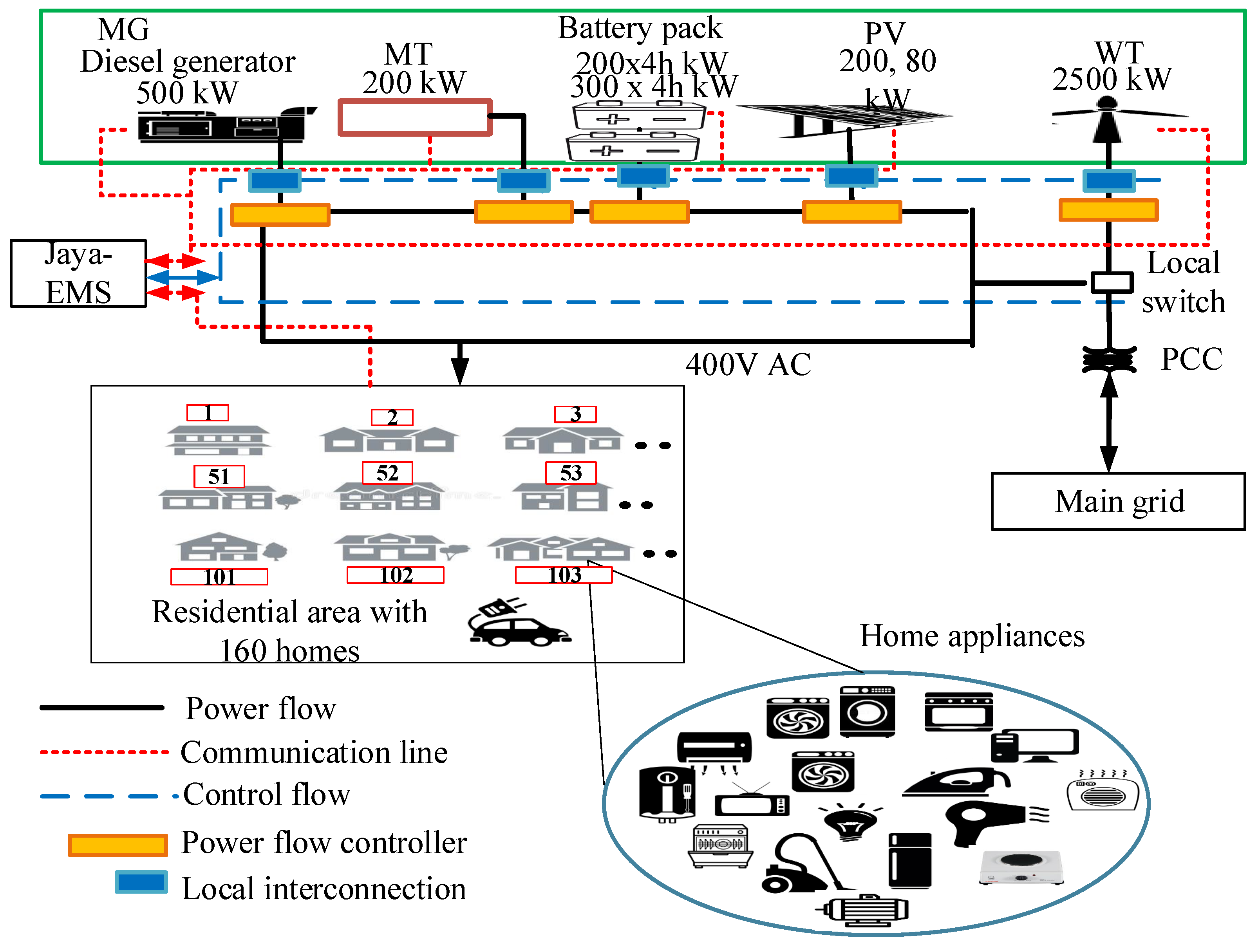
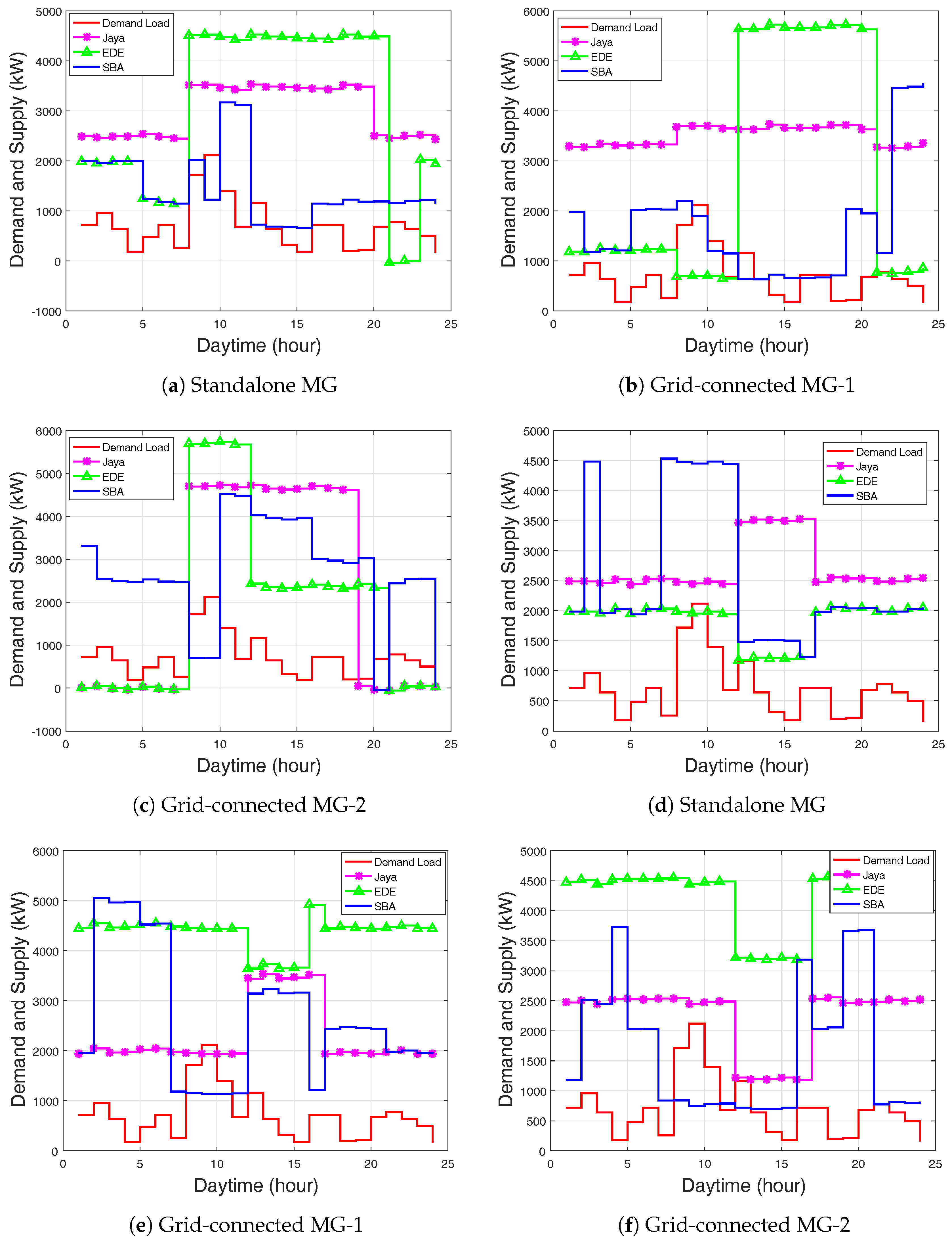
Figure 3 shows the hourly rating of DGs and the load demand. Load demand is the hourly aggregated operational loads of multiple homes. The figure shows that demand load is far greater than the initial power capacity of each distributed generation unit.

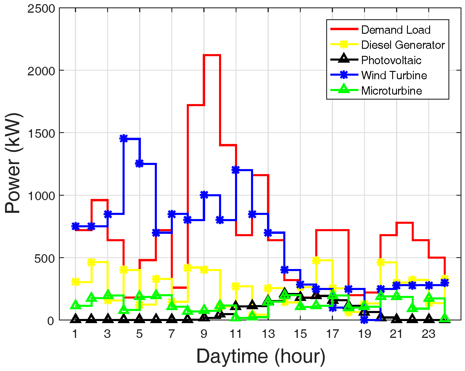
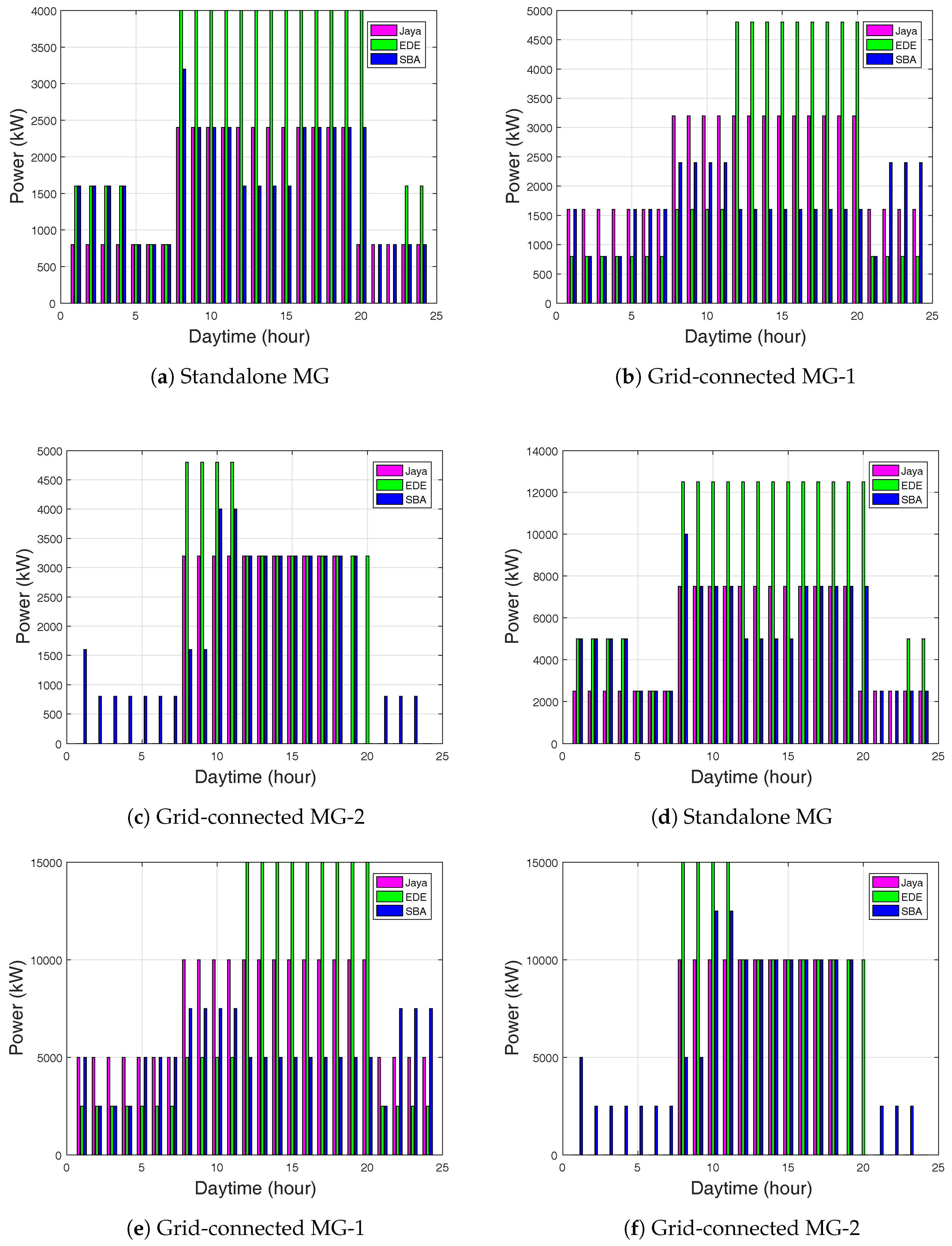
Optimal energy management for a MG with hourly ESU and SOC are shown in Figure 4, Figure 5 and Figure 6. In the ToU case for battery-1: During the first 7 h (12 a.m.–6 a.m.) of the simulation period for the ESU, the Jaya-based EMS stored the power of 3500 kW for 9–19 h and reduced in subsequent hours. EDE stored the power of 7200 kW, whereas the SBA-based EMS stored 6000 kW, as shown in Figure 4a for the standalone grid. The Jaya-based EMS stored the power of 4800 kW, whereas the EDE-based EMS stored 7200 kW and the SBA-based EMS stored 3200 kW, as shown in Figure 4b for grid-connected MG-1. In Figure 4c, the Jaya-based EMS stored the power of 4800 kW and EDE-based EMS stored 7200 kW, whereas, SBA-based EMS stored 6000 kW for grid-connected MG-2.

For the CPP case: 3500 kW was the stored power for Jaya, EDE, and SBA-based EMS, as shown in Figure 4d for the standalone grid. The stored power for Jaya in grid-connected MG-1 was 3500 kW, it was 6000 kW for EDE, and was 4800 kW SBA-based EMS, as shown in Figure 4e. Similarly, 3600 kW was the stored power of Jaya, EDE, and SBA-based EMS as shown in Figure 4f for grid-connected MG-2.

In battery-2, Jaya-based stored the power of 2800 kW, EDE-based stored 4000 kW, and SBA stored 3300 kW, as shown in Figure 5a for the standalone grid. In Figure 5b, Jaya-based stored the power of 3200 kW, EDE-based stored 4600 kW, and SBA-based EMS stored 2800 kW for for the grid-connected MG-1. Jaya-based EMS stored the power of 3200 kW, EDE-based stored 4700 kW, and SBA-based stored 4000 kW for the grid-connected MG-2. However, Jaya-based did not show stored power in some hours, because Jaya-based EMS sufficiently satisfied load demand.

In Figure 5d, the diesel generator for the standalone showed that Jaya-based EMS reduced its power supply during the first 1–9 h as compared to EDE and SBA. The maximum power supply of the diesel generator for Jaya-based EMS was 6800 kW, as compared to 12,200 kW for EDE and SBA. The maximum diesel power generation was 10,000 kW, as compared to 15,000 kW for EDE and SBA, as shown in Figure 5e. Similarly, for the Jaya-based EMS, the maximum diesel power generation was 10,000 kW, as compared to 15,000 kW for EDE and SBA (Figure 5f). However, the Jaya-based EMS had no diesel power supply during first 1–9 h and 19–24 h respectively. This is because the stored power in the batteries was used to satisfy the demand load request during these hours.

The batteries had unstable charging behavior due to the high demand load request. Figure 6a shows the SOC for the two MG operational modes. Meanwhile, the batteries maximum charging rates were 99% for SBA, 96% for Jaya, and 95% for EDE. There was no charging rate below the initially charged limit, and the MG could meet the load requirement even for the inactive state.

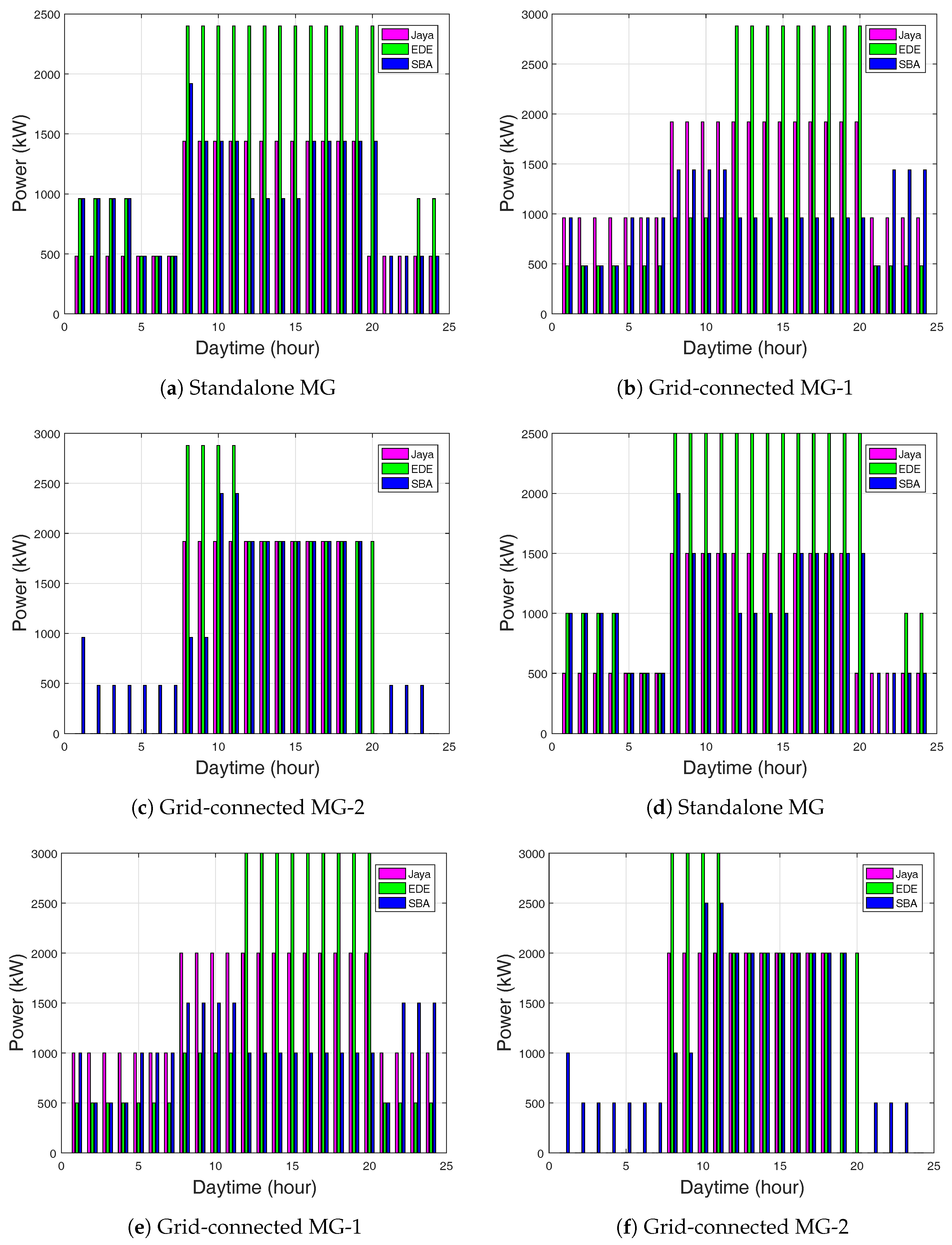
The PV unit significantly supplied 2500 kW power more than the 2400 kW of WT and 1000 kW of MT, as shown in Figure 7a and Figure 8a. SBA and EDE supplied more power in the WT unit than Jaya-based EMS. Figure 8d shows the maximum power supply of 2000 kW, 2500 kW, and 1500 kW of PV for SBA, EDE, and Jaya-based EMS, respectively. In this period, the MG could satisfy the load requirement and charged the batteries. The diesel generator unit supplied power of 12,200 kW as compared to the 8000 kW of battery-1 and 4000 kW of battery-2. Thus, fuel cost increased.

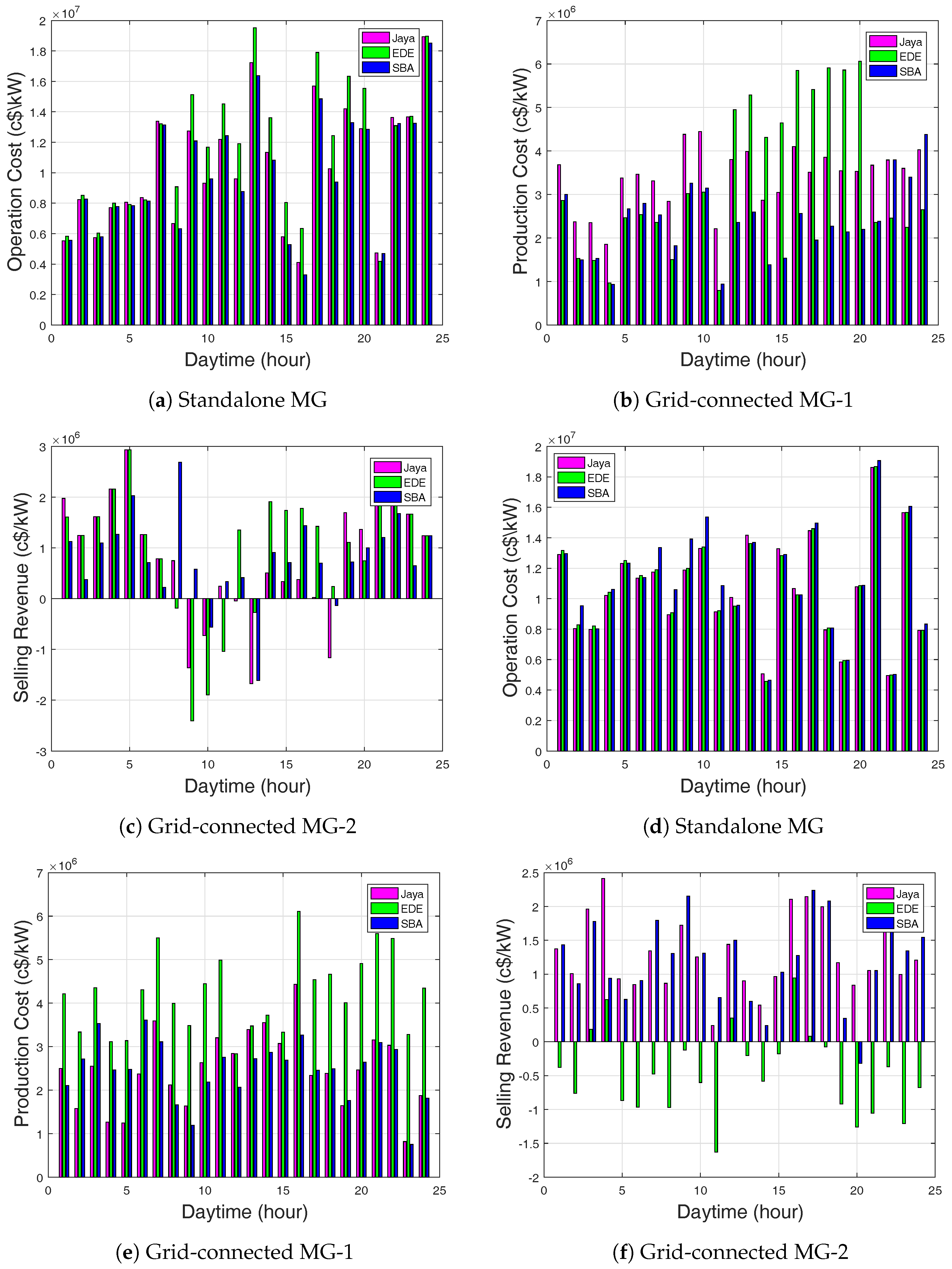
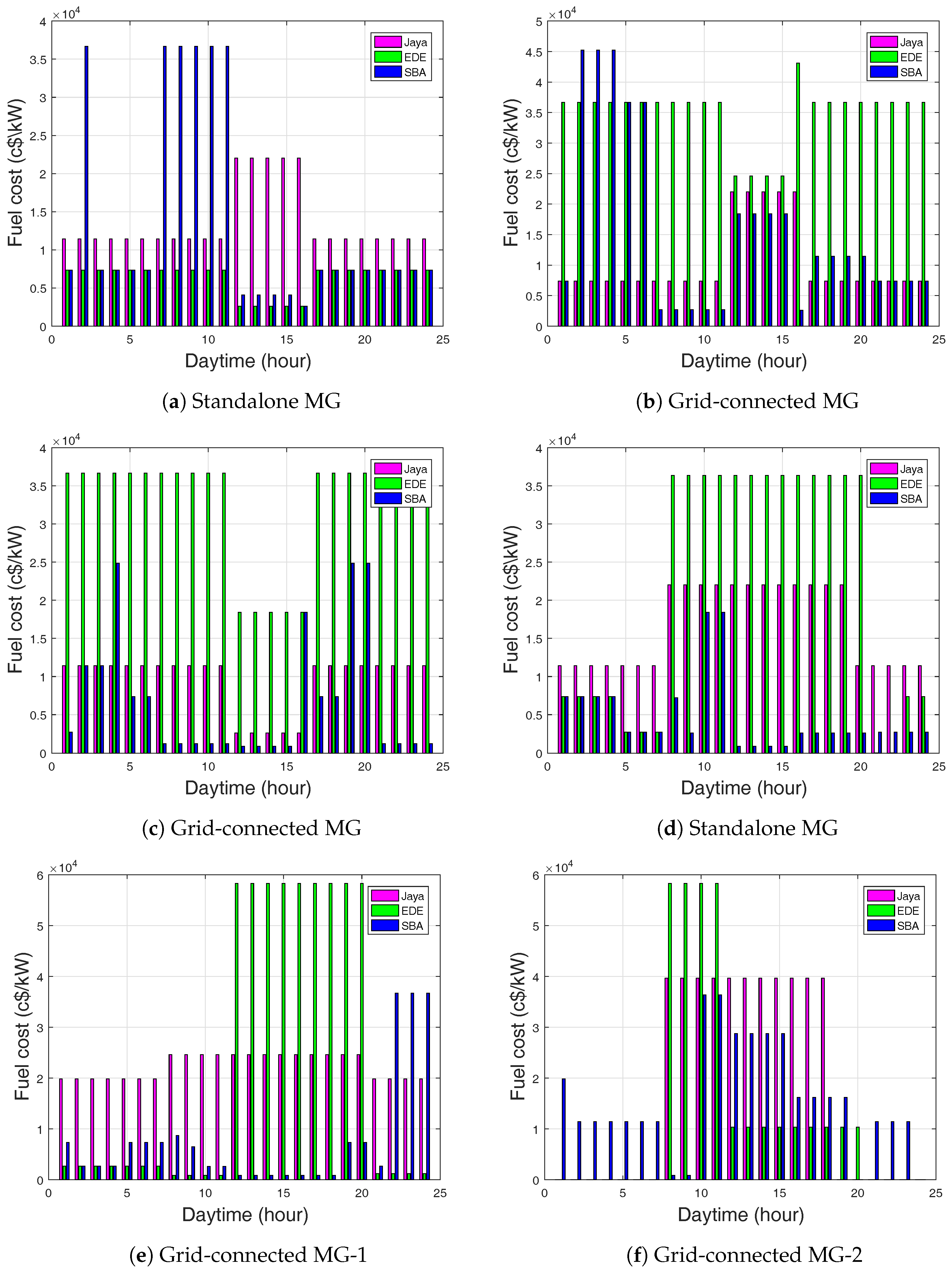
In Figure 9a, EDE-based EMS generated a minimal fuel cost in the first 7 h and was then reduced in the 12–16 h of the day, whereas SBA-based EMS generated the greatest fuel cost. In

Table 8. Fuel, production cost, and selling income by proposed methods using CPP scheme.

Standalone Grid
Optim. Model	Total Daily Fuel Cost (c$/kWh)	Daily Energy Selling Profit (c$/kWh)	Total Daily Production Cost (c$/kWh)	Computational Time (s)
Without EMS	403,850	13,325,000	4,2495,000	-
Jaya	327,280	31,027,000	2,600,500	0.4505
EDE	152,800	31,125,000	3,015,600	0.8126
SBA	334,610	−60,302,000	2,686,000	0.5172
Grid-connected MG-1
Jaya	249,840	23,023,000	2,600,500	0.0488
EDE	838,520	−18,478,000	3,015,600	0.3275
SBA	381,320	−65,229,000	2,686,000	0.2598
Grid-connected MG-2
Jaya	230,240	31,503,000	2,593,600	0.0575
EDE	789,070	−11,099,000	3,015,400	0.3371
SBA	162,600	−51,486,000	2,616,500	0.2316

, EDE-based EMS produced a sales revenue that was greater than that of Jaya and SBA. This is due to the high power supply of MT and PV. EDE-based EMS had minimal production cost as compared to Jaya and SBA.

Figure 9d shows the hourly fuel cost. The figure shows the time period with minimal fuel cost generated by SBA and Jaya-based EMS. All algorithms generated a high fuel cost during the peak hours which then reduced in subsequent hours. This was due to the high amount of power supplied by the diesel generator.

Figure 10a illustrates that there was a fluctuating cost of operations during the period of simulation. The results indicate that the EMS was able to shift dispatchable DGs from on-peak to off-peak hours. Table 8 and

Table 9. Fuel, production cost, and selling income of proposed methods using the ToU scheme.

Standalone Grid
Optim. Model	Total Hourly Fuel Cost (c$/kWh)	Total Hourly Energy Selling Profit (c$/kWh)	Total Daily Production Cost (c$/kWh)	Computational Time (s)
Without EMS	403,850	13,611,000	42,593,000	-
Jaya	401,380	22,376,000	24,998,000	0.4253
EDE	524,930	−7,369,700	27,972,000	0.6791
SBA	111,560	−45,810,000	24,157,000	0.5479
Grid-connected MG-1
Jaya	537,750	15,945,000	3,255,200	0.0977
EDE	552,070	17,002,000	3,244,600	0.3641
SBA	191,690	−5,992,000	3,056,600	0.2736
Grid-connected MG-2
Jaya	436,290	19,398,000	2,691,000	0.0551
EDE	326,570	23,644,000	2,652,800	0.3725
SBA	376,930	−61,490,000	2,697,000	0.3507

show the total daily fuel cost, production cost, and selling revenue for the ToU and CPP. In Table 9, EDE-based EMS showed a high total daily fuel cost of 5,24,930 USD cents per kilowatt-hour (c$/kWh) as compared to Jaya and SBA, meaning that there was a high production cost for Jaya and SBA. Jaya-based EMS showed better sales revenue than EDE and SBA. However, Jaya-based EMS showed minimum execution time as compared to SBA and EDE.

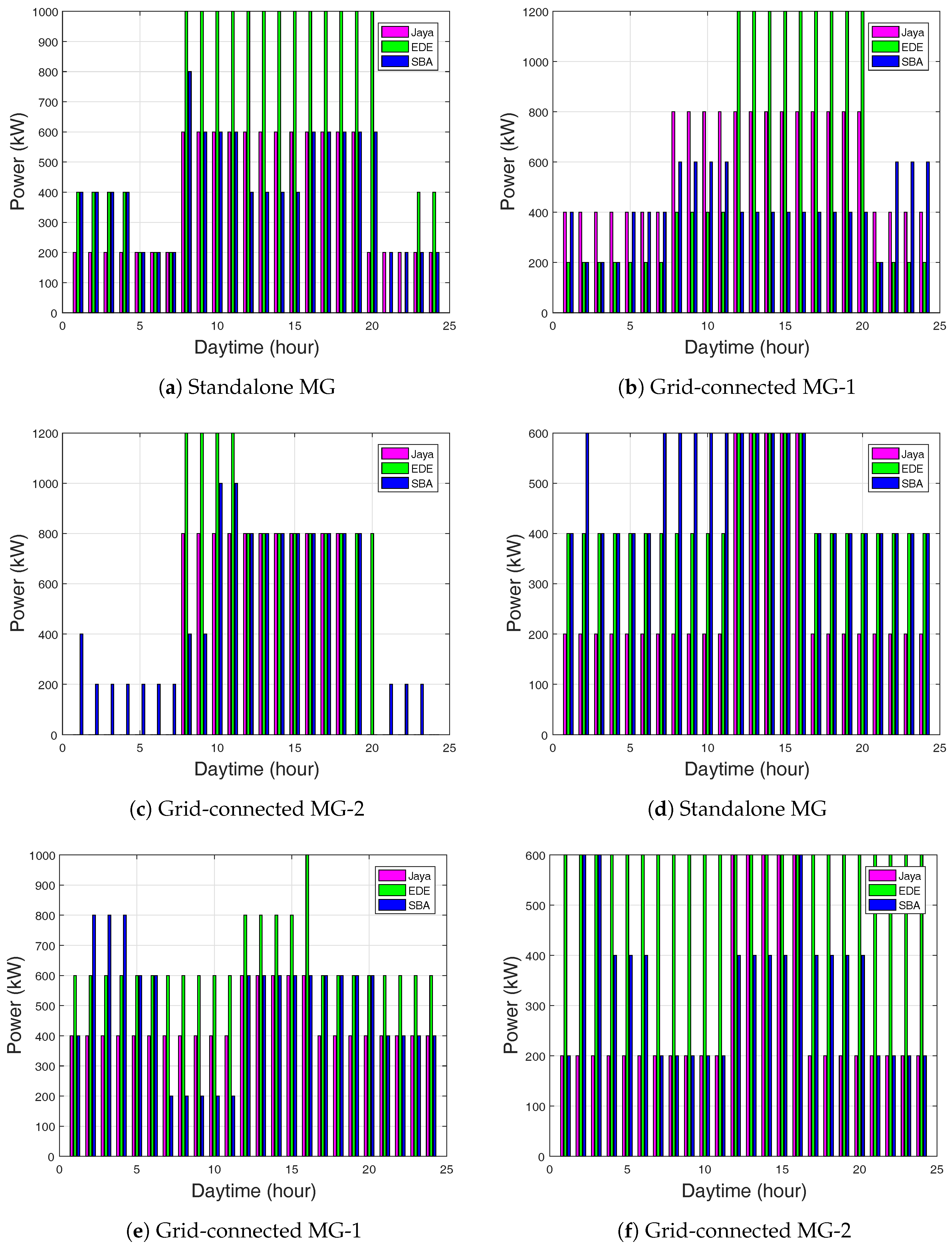
In Figure 11a during the first 8 h for Jaya and EDE-based EMS, a constant amount of power was supplied which sufficiently satisfied the load requirement. There was no reduction in power supply except for EDE-based EMS during hours 21 and 22. Thus, the batteries started discharging to supply power. During the peak hours, a high amount of power was supplied to satisfy the load request, and thus the batteries started charging.

For the CPP case, during the time periods of 1–11 h, Jaya-based EMS had continuous power stored at 1200 kW for battery-1 and 550 kW for battery-2. EDE and SBA-based EMS showed better power stored than the Jaya-based EMS with the power stored at 2400 kW for battery-1 and 1600 kW for battery-2. The power stored for all proposed algorithms was 3600 kW and 2400 kW for battery-1 and battery-2, respectively. The batteries had unsteady charging behavior, and this was due to high demand load request from the residential area. However, batteries did not get complete charging; more so, the batteries’ discharging did not exceed the specified charged limit of 20%. Thus, the MG could meet the demand load requirement of the residential area for the inactive state. In Figure 10d, SBA-based EMS produced the highest operating cost, greater than EDE and Jaya, respectively. The operation and maintenance costs were stable for the three algorithms, among which Jaya-based EMS had the minimal cost.

Operation in Grid-Connected Mode

In the grid-connected mode, energy exchange occurs between the MG and the main grid to meet the demand load requirement of the residential area. The EMS provides optimal scheduling of the DERs under grid-connected mode to minimize the production cost and maximize the sales revenue. Figure 11b shows demand and supply. The batteries were at steady charging state with the power stored of 8000 kW and 4000 kW for both grid-connected MG-1 and MG-2, as shown in Figure 4 and Figure 5.

The batteries stored more power for EDE than Jaya and SBA-based EMS. In the WT unit in Figure 8b,c, EDE-based EMS supplied more power than Jaya and SBA. The diesel generator power supply tended to reduce in Jaya and SBA, but was high for EDE-based EMS. In EDE-based EMS, the diesel generator incurred more fuel cost, since it generated 15,000 kW of power at 12–20 h and 15,000 kW at 8–12 h, as shown in Figure 9e.

As soon as the MG is able to meet demand load requirement of the residential area, batteries stop discharging for subsequent use during peak demand load request. In Figure 10c, SBA-based EMS did not show improvement in total daily production cost. If the power supplied is more from the MG than the power supplied by the main grid, then the preserved power from the ESSs can be used, especially when utility prices are high. The preferred performance of Jaya-based EMS over SBA and EDE in terms of sales revenues is clearly seen.

In the case of CPP, Jaya-based EMS in Table 8 had a minimum total daily production cost as compared to EDE and SBA. Figure 11e,f show the demand and supply for the grid-connected modes. From the figures, the MG supplied more power during the on-peak and off-peak hours. EDE-based EMS supplied more power as compared to Jaya and SBA. This is because EDE-based EMS scheduled the WT and MT at the same time. The negative selling revenue indicates the operation and maintenance costs were greater than the production cost.

5.2. Performance Trade-Off

To show the comparative analysis using CPP, the fuel cost without EMS was 403,850 c$/kWh. Jaya-based EMS reduced the daily fuel cost by up to 18.96% compared to the 62.16% of EDE and 17.14% of SBA for the standalone MG. Whereas, a daily fuel cost reduction of 38.13% was observed in the Jaya-based system compared to −107.63% in EDE and 5.57% in SBA for grid-connected MG-1. Additionally, Jaya-based EMS reduced fuel costs by up to 42.98% compared to −95.38% for EDE and 59.73% for SBA for the grid-connected MG-2. The total daily production cost without EMS was 42,495,000 c$/kWh; with Jaya-based EMS the total daily production cost was reduced by up to 93.89% compared to 92.90% with EDE and 93.67% with SBA for the standalone MG. Whereas, the daily production reduction with the Jaya-based EMS was 93.89% compared to 92.90% with EDE and 93.67% with SBA. In addition, Jaya-based EMS reduced the daily production cost by up to 93.89% compared to 92.90% for EDE and 93.84% of SBA for the grid-connected MG-1 and MG-2, respectively. The daily sales revenue without EMS was 13,325,000 c$/kWh; Jaya-based EMS achieved a maximum daily sales revenue above 100% (i.e., 132.84%) compared to 133.58% for EDE and −352.54% for SBA for the standalone MG. Whereas, the Jaya-based EMS maximized the daily sales revenue by up to 72.78% as compared to −38.67% for EDE and −389.52% for SBA. In addition, Jaya-based EMS maximized the daily sales revenue by up to 136.42% compared to −16.70% for EDE and −286.38% for SBA for grid-connected MG-1 and MG-2, respectively.

The following is a comparative analysis using ToU. The daily fuel cost without EMS was 403,850 c$/kWh; Jaya-based EMS reduced the daily fuel cost by up to 0.61% compared to −29.98% for EDE and 72.37% for SBA in the standalone MG. The Jaya-based EMS did not improve the daily fuel cost, with −33.15% compared to −36.70% with EDE and 52.53% with SBA. In a similar manner, Jaya-based EMS failed by −8.03% compared to 19.13% by EDE and 6.66% by SBA for the grid-connected MG-1 and MG-2 respectively. The total daily production costs without EMS were 42,593,000 c$/kWh; the total daily production cost with Jaya-based EMS was minimized by up to 41.30% compared to 34.32% with EDE and 43.28% with SBA for the standalone MG. Meanwhile, there was a 92.35% daily production cost reduction by Jaya-based EMS, compared to 92.38% by EDE and 92.82% by SBA. In addition, Jaya-based EMS reduced the daily production cost by up to 93.68% compared to 93.77% with EDE and 93.66% with SBA for the grid-connected MG-1 and MG-2 respectively. The daily sales revenue without EMS was 13,611,000 c$/kWh; Jaya-based EMS maximized the daily sales revenue by up to 64.39% compared to −45.85% with EDE and −236.56% with SBA for the standalone MG. Whereas, Jaya-based EMS maximized the daily sales revenue by up to 17.14% compared to 24.91% with EDE and −55.97% with SBA. Additionally, Jaya-based EMS maximized the daily sales revenue by up to 42.51% compared to 73.71% of EDE and −351.76% of SBA for grid-connected MG-1 and MG-2 respectively.

However, Jaya-based EMS outperformed the other methods in terms of execution time, having (0.4253, 0.0977, 0.0551) compared to (0.6791, 0.3641, 0.3725) with EDE and (0.5479, 0.2736, 0.3507) with SBA for standalone, grid-connected MG-1, and MG-2, respectively in the ToU case. Similarly, Jaya-based EMS showed better execution times of (0.4505, 0.0488, 0.0575) compared to (0.8126, 0.3275, 0.3371) for EDE and (0.5172, 0.2598, 0.2316) for SBA for standalone, grid-connected MG-1, and MG-2, respectively, in the CPP case.

6. Conclusions and Future Work

With the growing demand for electricity, it becomes necessary to integrate RESs with traditional grid sources in order to meet the requirements. MGs offer a way of incorporating various DERs by optimizing the monetary operation and control problem, resulting in efficient power utilization. In this paper, we used a multi-objective approach in scheduling various DERs to achieve minimized operation and maintenance costs. We formulated a multi-objective scheduling problem for the standalone and grid-connected operational modes under the CPP and ToU scheduling horizons. Furthermore, we applied the Jaya algorithm to the formulated problems to evaluate its effectiveness. Simulation results showed the best performance of Jaya against SBA and EDE methods in terms of production cost, fuel cost, selling revenue, and execution time.

Jaya-based EMS reduced the total daily fuel cost by up to 38.13% as compared to EDE and SBA. Additionally, the total daily production cost of the Jaya-based EMS was reduced by up to 93.89% as compared to EDE and SBA. Moreover, Jaya-based EMS achieved a maximum daily sales revenue above 100% (i.e., 132.84%) as compared to EDE and SBA. Additionally, Jaya-based EMS outperformed the other methods in terms of execution time (0.4253 s).

The current MG operations can be modelled as a multi-objective scheduling problem, which can be effectively solved using the proposed approach. Our future work will aim at determining the size of the MG, as well robustness to communication outages and addressing prevalent security threats within the network.

References

1. Li, H.; Eseye, A.T.; Zhang, J.; Zheng, D. Optimal energy management for industrial microgrids with high-penetration renewables. Prot. Control Mod. Power Syst. 2017, 2, 12. [Google Scholar] [CrossRef]
2. Zachar, M.; Daoutidis, P. Microgrid/macrogrid energy exchange: A novel market structure and stochastic scheduling. IEEE Trans. Smart Grid 2017, 8, 178–189. [Google Scholar] [CrossRef]
3. Mehdizadeh, A.; Taghizadegan, N. Robust optimisation approach for bidding strategy of renewable generation-based microgrid under demand side management. IET Renew. Power Gener. 2017, 11, 1446–1455. [Google Scholar] [CrossRef]
4. Zhang, X. Optimal scheduling of critical peak pricing considering wind commitment. IEEE Trans. Sustain. Energy 2014, 5, 637–645. [Google Scholar] [CrossRef]
5. Celebi, E.; Fuller, J.D. Time-of-use pricing in electricity markets under different market structures. IEEE Trans. Power Syst. 2012, 27, 1170–1181. [Google Scholar] [CrossRef]
6. Abhinav, S.; Schizas, I.D.; Ferrese, F.; Davoudi, A. Optimization-Based AC Microgrid Synchronization. IEEE Trans. Ind. Inform. 2017, 13, 2339–2349. [Google Scholar] [CrossRef]
7. Dehghanpour, K.; Nehrir, H. Real-time multiobjective microgrid power management using distributed optimization in an agent-based bargaining framework. IEEE Trans. Smart Grid 2017. [Google Scholar] [CrossRef]
8. Liu, J.; Chen, H.; Zhang, W.; Yurkovich, B.; Rizzoni, G. Energy management problems under uncertainties for grid-connected microgrids: A chance constrained programming approach. IEEE Trans. Smart Grid 2017, 8, 2585–2596. [Google Scholar] [CrossRef]
9. Luo, Z.; Wu, Z.; Li, Z.; Cai, H.; Li, B.; Gu, W. A two-stage optimization and control for CCHP microgrid energy management. Appl. Therm. Eng. 2017, 125, 513–522. [Google Scholar] [CrossRef]
10. Moga, D.; Petreuş, D.; Mureşan, V.; Stroia, N.; Cosovici, G. Optimal generation scheduling in islanded microgrids. IFAC-PapersOnLine 2016, 49, 135–139. [Google Scholar] [CrossRef]
11. Chen, J.; Chen, J. Stability Analysis and Parameters Optimization of Islanded Microgrid with Both Ideal and Dynamic Constant Power Loads. IEEE Trans. Ind. Electron. 2017, 65, 3263–3274. [Google Scholar] [CrossRef]
12. Su, W.; Wang, J.; Roh, J. Stochastic energy scheduling in microgrids with intermittent renewable energy resources. IEEE Trans. Smart Grid 2014, 5, 1876–1883. [Google Scholar] [CrossRef]
13. Shuai, H.; Fang, J.; Ai, X.; Tang, Y.; Wen, J.; He, H. Stochastic Optimization of Economic Dispatch for Microgrid Based on Approximate Dynamic Programming. IEEE Trans. Smart Grid 2018. [Google Scholar] [CrossRef]
14. Razmara, M.; Bharati, G.R.; Shahbakhti, M.; Paudyal, S.; Robinett, RD., III. Bilevel optimization framework for smart building-to-grid systems. IEEE Trans. Smart Grid 2016, 9, 582–593. [Google Scholar] [CrossRef]
15. Esfahani, M.M.; Hariri, A.; Mohammed, O.A. A Multiagent-based Game-Theoretic and Optimization Approach for Market Operation of Multi-Microgrid Systems. IEEE Trans. Ind. Inform. 2018. [Google Scholar] [CrossRef]
16. Rao, R.V.; Waghmare, G.G. A new optimization algorithm for solving complex constrained design optimization problems. Eng. Optim. 2017, 49, 60–83. [Google Scholar] [CrossRef]
17. Fang, X.; Yang, Q.; Dong, W. Fuzzy decision based energy dispatch in offshore industrial microgrid with desalination process and multi-type DGs. Energy 2018, 148, 744–755. [Google Scholar] [CrossRef]
18. Naderi, M.; Bahramara, S.; Khayat, Y.; Bevrani, H. Optimal planning in a developing industrial microgrid with sensitive loads. Energy Rep. 2017, 3, 124–134. [Google Scholar] [CrossRef]
19. Stevanoni, C.; De Grève, Z.; Vallée, F.; Deblecker, O. Long-term Planning of Connected Industrial Microgrids: A Game Theoretical Approach Including Daily Peer-to-Microgrid Exchanges. IEEE Trans. Smart Grid 2018. [Google Scholar] [CrossRef]
20. Comodi, G.; Giantomassi, A.; Severini, M.; Squartini, S.; Ferracuti, F.; Fonti, A.; Cesarini, D.N.; Morodo, M.; Polonara, F. Multi-apartment residential microgrid with electrical and thermal storage devices: Experimental analysis and simulation of energy management strategies. Appl. Energy 2015, 137, 854–866. [Google Scholar] [CrossRef]
21. Pascual, J.; Barricarte, J.; Sanchis, P.; Marroyo, L. Energy management strategy for a renewable-based residential microgrid with generation and demand forecasting. Appl. Energy 2015, 158, 12–25. [Google Scholar] [CrossRef]
22. Zhang, X.; Karady, G.G.; Guan, Y. Design methods investigation for residential microgrid infrastructure. Int. Trans. Electr. Energy Syst. 2011, 21, 2125–2141. [Google Scholar] [CrossRef]
23. Kriett, P.O.; Salani, M. Optimal control of a residential microgrid. Energy 2012, 42, 321–330. [Google Scholar] [CrossRef]
24. Das, A.; Ni, Z. A Computationally Efficient Optimization Approach for Battery Systems in Islanded Microgrid. IEEE Trans. Smart Grid 2017. [Google Scholar] [CrossRef]
25. Tasdighi, M.; Ghasemi, H.; Rahimi-Kian, A. Residential microgrid scheduling based on smart meters data and temperature dependent thermal load modeling. IEEE Trans. Smart Grid 2014, 5, 349–357. [Google Scholar] [CrossRef]
26. Corchero, C.; Cruz-Zambrano, M.; Heredia, F.J. Optimal energy management for a residential microgrid including a vehicle-to-grid system. IEEE Trans. Smart Grid 2014, 5, 2163–2172. [Google Scholar]
27. Zhang, Y.; Zhang, T.; Wang, R.; Liu, Y.; Guo, B. Optimal operation of a smart residential microgrid based on model predictive control by considering uncertainties and storage impacts. Sol. Energy 2015, 122, 1052–1065. [Google Scholar] [CrossRef]
28. Liu, G.; Xu, Y.; Tomsovic, K. Bidding strategy for microgrid in day-ahead market based on hybrid stochastic/robust optimization. IEEE Trans. Smart Grid 2016, 7, 227–237. [Google Scholar] [CrossRef]
29. Borghetti, A.; Bosetti, M.; Grillo, S.; Massucco, S.; Nucci, C.A.; Paolone, M.; Silvestro, F. Short-term scheduling and control of active distribution systems with high penetration of renewable resources. IEEE Syst. J. 2010, 4, 313–322. [Google Scholar] [CrossRef]
30. Liu, G.; Starke, M.; Xiao, B.; Tomsovic, K. Robust optimisation-based microgrid scheduling with islanding constraints. IET Gener. Transm. Distrib. 2017, 11, 1820–1828. [Google Scholar] [CrossRef]
31. Cao, X.; Wang, J.; Zeng, B. A Chance Constrained Information-Gap Decision Model for Multi-Period Microgrid Planning. IEEE Trans. Power Syst. 2017, 33, 2684–2695. [Google Scholar] [CrossRef]
32. Farzin, H.; Fotuhi-Firuzabad, M.; Moeini-Aghtaie, M. A stochastic multi-objective framework for optimal scheduling of energy storage systems in microgrids. IEEE Trans. Smart Grid 2017, 8, 117–127. [Google Scholar] [CrossRef]
33. Chiş, A.; Koivunen, V. Coalitional game based cost optimization of energy portfolio in smart grid communities. IEEE Trans. Smart Grid 2017. [Google Scholar] [CrossRef]
34. Li, Y.Z.; Wang, P.; Gooi, H.B.; Ye, J.; Wu, L. Multi-Objective Optimal Dispatch of Microgrid under Uncertainties via Interval Optimization. IEEE Trans. Smart Grid 2017. [Google Scholar] [CrossRef]
35. Li, D.; Hongjian, S.U.; Chiu, W.Y.; Poor, H.V. Multiobjective Optimization for Demand Side Management in Smart Grid. IEEE Trans. Ind. Inform. 2017, 14, 1482–1490. [Google Scholar] [CrossRef]
36. Roggia, L.; Schuch, L.; Baggio, J.E.; Rech, C.; Pinheiro, J.R. Integrated full-bridge-forward DC–DC converter for a residential microgrid application. IEEE Trans. Power Electron. 2013, 28, 1728–1740. [Google Scholar] [CrossRef]
37. Kinhekar, N.; Padhy, N.P.; Li, F.; Gupta, H.O. Utility oriented demand side management using smart AC and micro DC grid cooperative. IEEE Trans. Power Syst. 2016, 31, 1151–1160. [Google Scholar] [CrossRef]
38. Khan, B.; Singh, P. Selecting a Meta-Heuristic Technique for Smart Micro-Grid Optimization Problem: A Comprehensive Analysis. IEEE Access 2017, 5, 13951–13977. [Google Scholar] [CrossRef]
39. Chakraborty, N.; Mondal, A.; Mondal, S. Efficient Scheduling of Non-Preemptive Appliances for Peak Load Optimization in Smart Grid. IEEE Trans. Ind. Inform. 2017. [Google Scholar] [CrossRef]
40. Nikmehr, N.; Najafi-Ravadanegh, S.; Khodaei, A. Probabilistic optimal scheduling of networked microgrids considering time-based demand response programs under uncertainty. Appl. Energy 2017, 198, 267–279. [Google Scholar] [CrossRef]
41. Warid, W.; Hizam, H.; Mariun, N.; Abdul-Wahab, N.I. Optimal power flow using the jaya algorithm. Energies 2016, 9, 678. [Google Scholar] [CrossRef]
42. Samuel, O.; Javaid, N.; Aslam, S.; Rahim, M.H. JAYA optimization based energy management controller. In Proceedings of the IEEE 2018 International Conference on Computing, Mathematics and Engineering Technologies (iCoMET), Sukkur, Pakistan, 3–4 March 2018; pp. 1–8. [Google Scholar]
43. Rao, R. Venkata. Jaya: A simple and new optimization algorithm for solving constrained and unconstrained optimization problems. Int. J. Ind. Eng. Comput. 2016, 7, 19–34. [Google Scholar]
44. Akyol, S.; Alatas, B. Plant intelligence based metaheuristic optimization algorithms. Artif. Intell. Rev. 2017, 47, 417–462. [Google Scholar] [CrossRef]
45. Merrikh-Bayat, F. A Numerical Optimization Algorithm Inspired by the Strawberry Plant. arXiv, 2014; arXiv:1407.7399. [Google Scholar]
46. Price, K.; Storn, R.M.; Lampinen, J.A. Differential Evolution: A Practical Approach to Global Optimization; Springer Science & Business Media: Berlin, Germany, 2006. [Google Scholar]
47. Time of Use Rates. Waterloo North Hydro Inc., 2017. Available online: https://www.wnhydro.com/en/your-home/time-of-use-rates.asp (accessed on 6 December 2017).
Figure 1. Proposed system model. EMS: energy management system; PCC: point of common coupling; PV: photovoltaic; WT: wind turbine.
Energies 11 01513 g001
Figure 2. Proposed architecture for Jaya-based EMS. BAT: battery.
Energies 11 01513 g002
Figure 3. Hourly demand load and rating of dispatchable DG.
Energies 11 01513 g003
Figure 4. Power stored using the battery-1: (a) Standalone MG using ToU; (b) Grid-connected MG-1 using ToU; (c) Grid-connected MG-2 using ToU; (d) Standalone MG using CPP; (e) Grid-connected MG-1 using CPP; (f) Grid-connected MG-2 using CPP.
Energies 11 01513 g004
Figure 5. (a) Power stored using battery-2 in standalone MG using ToU; (b) Power stored using battery-2 in grid-connected MG-1 using ToU; (c) Power stored using battery-2 in grid-connected MG-2 using ToU; (d) Power generation using the diesel generator in standalone MG using ToU; (e) Power generation using the diesel generator in grid-connected MG-1 using ToU; (f) Power generation using the diesel generator in grid-connected MG-2 using ToU.
Energies 11 01513 g005
Figure 6. (a) SOC in standalone MG using ToU; (b) SOC in grid-connected MG-1 using ToU; (c) SOC in grid-connected MG-2 using ToU; (d) SOC in standalone MG using CPP; (e) SOC in grid-connected MG-1 using CPP; (f) SOC in grid-connected MG-2 using CPP.
Energies 11 01513 g006
Figure 7. (a) Power generation for MT in standalone MG using ToU; (b) Power generation for MT in grid-connected MG-1 using ToU; (c) Power generation for MT in grid-connected MG-2 using ToU; (d) Power generation for MT in standalone MG using CPP; (e) Power generation for MT in grid-connected MG-1 using CPP; (f) Power generation for MT in grid-connected MG-2 using CPP.
Energies 11 01513 g007
Figure 8. (a) Power generation for WT in standalone MG using ToU; (b) Power generation for WT in grid-connected MG-1 using ToU; (c) Power generation for WT in grid-connected MG-2 using ToU; (d) Power generation for PV in standalone MG using ToU; (e) Power generation for PV in grid-connected MG-1 using ToU; (f) Power generation for PV in grid-connected MG-2 using ToU.
Energies 11 01513 g008
Figure 9. (a) Diesel fuel consumption cost in standalone MG using CPP; (b) Diesel fuel consumption cost in grid-connected MG-1 using CPP; (c) Diesel fuel consumption cost in grid-connected MG-2 using CPP; (d) Diesel fuel consumption cost in standalone MG using ToU; (e) Diesel fuel consumption cost in grid-connected MG-1 using ToU; (f) Diesel fuel consumption cost in grid-connected MG-2 using ToU.
Energies 11 01513 g009
Figure 10. (a) Operation and maintenance cost using ToU; (b) Production cost using ToU; (c) Selling revenue using ToU; (d) Operation and maintenance using CPP; (e) Production cost using CPP; (f) Selling revenue using CPP.
Energies 11 01513 g010
Figure 11. (a) Demand and supply in standalone MG using ToU; (b) Demand and supply in grid-connected MG-1 using ToU; (c) Demand and supply in grid-connected MG-2 using ToU; (d) Demand and supply in standalone MG using CPP; (e) Demand and supply in grid-connected MG-1 using CPP; (f) Demand and supply in grid-connected MG-2 using CPP.
Energies 11 01513 g011