Scenario Analysis of Carbon Emissions of Beijing-Tianjin-Hebei

Abstract

This paper utilizes the generalized Fisher index (GFI) to decompose the factors of carbon emission and exploits improved particle swarm optimization-back propagation (IPSO-BP) neural network modelling to predict the primary energy consumption CO₂ emissions in different scenarios of Beijing-Tianjin-Hebei region. The results show that (1) the main factors that affect the region are economic factors, followed by population size. On the contrary, the factors that mainly inhibit the carbon emissions are energy structure and energy intensity. (2) The peak year of carbon emission changes with the different scenarios. In a low carbon scenario, the carbon emission will have a decline stage between 2015 and 2018, then the carbon emission will be in the ascending phase during 2019–2030. In basic and high carbon scenarios, the carbon emission will peak in 2025 and 2028, respectively.

1. Introduction

Global warming is a hot topic in the world, and the issue of carbon emission has attracted extensive attention worldwide. China made its own contributions in the Paris Agreement, which were that the CO₂ emissions will peak in 2030, and the carbon emission intensity will decrease by 60–65% based on 2005 [1]. Currently, China is the largest carbon emission country in the world, and the carbon emission of the Beijing-Tianjin-Hebei region is about one fifth of the emissions from China. At the same time, the population of the region has exceeded 100 million, and it is facing serious ecological problems [2].

Beijing-Tianjin-Hebei region is defined as the “Capital Circle” of China. Beijing is the capital of China, it is also an international metropolis and a center for science and technology innovation. Tianjin is one of the first coastal open cities, it has essential ports. Hebei is an important grain and cotton production region of China, which is rich in resources [3]. In 2004, the National Development and Reform Commission (NDRC) proposed a “langfang consensus” on some principles of economic integration of Beijing-Tianjin-Hebei region [4]. In 2006, the development of Beijing-Tianjin-Hebei region was included in the “11th five-year plan” [5]. In 2011, the “12th five-year plan” was released, and the concept of “capital economic circle“ was built. In 2016, the Supreme People’s Court promulgated the documents of “The legal services of the supreme people’s court on the coordinated development of Beijing-Tianjin-Hebei”, which was put forward to guarantee the development concepts [6]. Thus, the Beijing-Tianjin-Hebei region is of significance to the environment and economic development in China.

The study of carbon emission in Beijing-Tianjin-Hebei region is very meaningful. Reference [7] established a Stochastic Impacts by Regression on Population, Affluence, and Technology (STIRPAT) model, and the study found that the principal factor which affected this region was the economic factors. Reference [8] adopted a mixed method to study the air pollution prevention and control action plan in Beijing-Tianjin-Hebei. Reference [9] constructed an internationally compatible method, and compared the differences of carbon emission between the urban and non-urban areas in industry, agriculture, households and transport. Reference [10] developed a life cycle footprint analysis method, and assessed the tourism-related direct and indirect water consumption under four scenarios in Beijing-Tianjin-Hebei region. Reference [11] undertook a study on the key energy-intensive industries of the Beijing-Tianjin-Hebei, and decomposed the factors by the Malmquist index, the research showed that the principal influence factor was technological progress. Reference [12] took an air pollutants emission inventory of Beijing-Tianjin-Hebei region, and analyzed the emission of different pollutants such as CO₂, SO₂, and NO_x in 2013. In order to study the energy-related CO₂ emissions in China, reference [13] used the Logarithmic Mean Divisia Index (LMDI) method to decompose the influencing factors. The results indicated that energy intensity had a positive effect on decreasing the CO₂ emissions. Therefore, we can conclude that, it is meaningful to study the Beijing-Tianjin-Hebei, especially, the primary energy-related carbon emissions of this region. This paper decomposed the influence factors of carbon emission by the Generalized Fisher Index (GFI), and predicted the energy-related CO₂ emissions in Beijing-Tianjin-Hebei region using the improved particle swarm optimization-back propagation (IPSO-BP) neural network model and scenario analysis methods.

2. Literature Review

There is considerable research about energy-related CO₂ emissions, and the factors that influence the CO₂ are different. Reference [14] used time series modelling to assess the relationship between foreign direct investment (FDI) and energy consumption. Relying on the Generalized Divisia Index, reference [15] decomposed the changes in the energy-related Greenhouse Gas (GHG) emissions. To analyze the relationship between the industrial structural transformation and carbon dioxide emissions, reference [16] applied panel data from 1995 to 2009, and found out the most effective way to reduce the emissions was industrial structural adjustment. Reference [17] employed a Renewable Energy Country Attractiveness Index, and investigated the effects of renewable energy consumption on the economic growth of major renewable energy consuming countries in the world. Reference [18] developed an allocation principle, which was based on the efficiency levels, and constructed the links between energy intensity and efficiency. Reference [19] established a Logarithmic Mean Divisia Index method, and analyzed the methods of controlling the coal consumption of three major CO₂ emitters. Reference [20] calculated the primary energy consumption and energy-related CO₂ emissions in five countries. These studies have shown that the influencing factors of the energy-related CO₂ emissions vary from country to country.

A large number of scholars have studied the methods of decomposing factors which influence carbon emissions, and the commonly used methods are structural decomposition method (SDA) and index decomposition analysis (IDA). The SDA method can be divided into two categories: decomposition method and input-output method. Currently, the IDA method can be divided into the Laspeyres index and the Divisia index. The main idea of Laspeyres index was proposed in the late 1970s, and has been further improved since then [21]. Reference [22] compared the difference between the Arithmetic Mean Divisia Index and Logarithmic Mean Divisia Index (LMDI). As a consequence, both methods agreed that the most important factor to the increase of CO₂ emissions was income effect. Reference [23] summarized the properties of the Divisia index and the Laspeyres index, meanwhile, the research provided recommendations when selecting the method. Reference [24] decomposed the factors into CO₂ emissions coefficient, technology effect, and change in final demand, it found that the main influencing factors were varied from time to time. A detailed review of the methods of decomposing factors is presented in

Table 1. Detailed review of the methods of decomposing factors.

Author(s)	Methodologies	Factors
[25]	Structural decomposition analysis (SDA)	structural change, technological improvements
[26]	Structural decomposition analysis (SDA)	GDP, Aggregate carbon intensity
[27]	Structural decomposition analysis (SDA) Generalized Fisher index(GFI)	Population, GDP, energy intensity
[28]	Structural decomposition analysis (SDA) Multiplicative decomposition	Total ratio changes, Emission intensity effect, Leontief structure effect, Domestic export effect
[29]	Structural decomposition analysis (SDA)	carbonization, energy intensity, technology, structural demand, consumption pattern and scale.
[30]	Structural decomposition analysis (SDA) Input-Output model	GDP, Population, energy intensity
[31]	Structural decomposition analysis (SDA) Index decomposition analysis (IDA)	energy intensity effect, Leontief effect, structure effect, affluence effect, population
[32]	Index decomposition analysis (IDA)	per capital income, energy prices, population growth, fossil fuel energy consumption, the investment capital ratio, country fixed effect
[33]	Index decomposition analysis (IDA)	activity effect, structure effect, sub-structure effect, intensity effect
[34]	index decomposition analysis (IDA) Advanced sustainability analysis	total primary energy supply, final energy consumption, GDP, population
[35]	Index Decomposition Analysis-Logarithmic Mean Divisia Index (IDA-LMDI)	carbonization, the substitution of fossil fuels, the penetration of renewable energy, energy intensity, wealth and population
[36]	Logarithmic Mean Divisia Index (LMDI)	activity, structural, energy intensity, fuel share, and emission effects
[37]	Logarithmic Mean Divisia Index (LMDI)	economic scale effect, industry structure effect, energy intensity effect, energy structure
[38]	Logarithmic Mean Divisia Index (LMD-I)	Inter-sector structural change, Per capital GDP change, Business energy intensity, Household energy intensity
[39]	Logarithmic Mean Divisia Index (LMDI)	cement output, clinker share, process structure, specific energy consumption
[40]	Logarithmic Mean Divisia Index (LMDI)	energy structure, energy intensity, industry structure, economic output, population scale effects

.

Many scholars have used different prediction methods to study CO₂ emissions. To forecast CO₂ emissions, reference [41] established an improved Gaussian processes regression method, which was based on a modified PSO algorithm proposed. Reference [42] proposed an improved particle swarm optimization-back propagation algorithm (IPSO-BP) method, and contrasted the result with the Grey prediction model GM(1,1) and a simple BP neural network. By applying Extreme Learning Machine (ELM), reference [43] predicted GDP based on emissions, and made a comparison with genetic programming (GP) and artificial neural networks (ANN). Reference [44] applied panel data to examine the relation between CO₂ emissions, renewable and non-renewable energy consumption, and economic growth. Reference [45] utilized the model of Equation specification and Panel cointegration approach to study the CO₂ emissions of renewable energy. By exploring the auto-regressive distributed lag (ARDL) model, reference [46] analyzed the validity of the Environmental Kuznets Curve (EKC) with the indicators of CO₂ emissions and the ecological footprint. Reference [47] built a hierarchical structure method, and verified the connection with CO₂ emissions and economic growth. Reference [48] predicted the CO₂ emission by using Support Vector Machine (SVM). Another important contribution of the study was that it compared the results with the Artificial Neural network (ANN) and Genetic Programming (GP) methods.

Most of the previous researches utilized structural decomposition method (SDA) or index decomposition analysis (IDA) when decomposing the factors. However, these models have certain defects, which cannot explain part of the changes in CO₂ emissions. Further, Fisher index method (GFI) can overcome the defects of these methods [49,50]. Meanwhile, those researches rarely considered the CO₂ emissions from energy consumption in Beijing-Tianjin-Hebei region. To compensate the defects of the existing studies, this paper applies the GFI model to analyze the influencing factors of energy consumption related CO₂ emissions, then combines the IPSO-BP neural network with scenario analysis to predict energy consumption related CO₂ emissions in Beijing-Tianjin-Hebei region during 2015–2030. The remainder of this study is organized as follows: Section 3 introduces the methods and data source of this research. Section 4 analyzes and discusses the empirical results. Finally, we draw a conclusion in Section 5.

3. Methods and Date Source

3.1. The Estimation of CO₂

This paper mainly studies the carbon dioxide produced by primary energy consumption in Beijing-Tianjin-Hebei, and the selected fossil fuels including coal, coke, crude oil, gasoline, kerosene, diesel oil, fuel oil, and natural gas. Conversion coefficient and CO₂ emissions conversion coefficient for various types of energy, which were recommended by the intergovernmental panel on climate change (IPCC) [51], are shown in

Table 2. Conversion coefficient and CO₂ emissions conversion coefficient of different kinds of energy.

Energy	Statistical Unit	Conversion Coefficient	CO2 Emissions Conversion Coefficient (C/(t/t))
Coal	million ton	0.7143 kgce/kg	0.747
Coke	million ton	0.9714 kgce/kg	0.855
Crude oil	million ton	1.4286 kgce/kg	0.585
Gasoline	million ton	1.4714 kgce/kg	0.553
Kerosne	million ton	1.4714 kgce/kg	0.571
DieSl oil	million ton	1.4571 kgce/kg	0.592
Fuel oil	million ton	1.4286 kgce/kg	0.618
Natural gas	billion cubic meters	1.2721 kgce/m3	0.448

. And the total carbon emissions produced by primary energy consumption can be calculated as Equation (1).

$$CE={\displaystyle \sum _{i=1}^9}{E}_i\ast C_i\ast K_{i\ast }\frac{12}{44}$$

(1)

where, CE represents the total of CO₂ emissions of primary energy consumption; i represents the fossil energy, involving coal, coke, crude oil, gasoline, kerosene, diesel oil, fuel oil, and natural gas; E_i represents the consumption of different kinds of energy; C_i and K_i represent conversion coefficient and CO₂ emissions conversion coefficient, respectively; 12/44 is the ratio between the mass of one carbon atom and the mass of one carbon dioxide molecule.

3.2. Generalized Fisher Index

The traditional calculation model of Fisher index decomposition is as Equation (2).

$$V={\displaystyle \sum _i{V}_i}={\displaystyle \sum _i{X}_{1i}}\cdot X_{2i},$$

(2)

where V denotes an indicator to be decomposed, and i is the subcategory of the indicator; and X_1i and X_2i represent the decomposed influencing factors. The effect associated with the changes in V from 0 year to T year can be decomposed into $D_{X_1}$ and $D_{X_2}$, the specific expression is presented as Equation (3).

$$V=\frac{V^T}{V^0}=\frac{{\displaystyle \sum _i{X_{1i}}^T\cdot {X_{2i}}^T}}{{\displaystyle \sum _i{X_{1i}}^0\cdot {X_{2i}}^0}}=D_{X_1}\cdot D_{X_2}$$

(3)

Based on the Fisher index model, $D_{X_1}$ and $D_{X_2}$ can be expressed as Equations (4) and (5).

$$D_{X_1}=\left[\frac{{\displaystyle \sum _i{X_{1i}}^T\cdot {X_{2i}}^0}}{{\displaystyle \sum _i{X_{1i}}^0\cdot {X_{2i}}^0}}\cdot \frac{{\displaystyle \sum _i{X_{1i}}^T\cdot {X_{2i}}^T}}{{\displaystyle \sum _i{X_{1i}}^0\cdot {X_{2i}}^T}}\right]$$

(4)

$$D_{X_2}=\left[\frac{{\displaystyle \sum _i{X_{1i}}^T\cdot {X_{2i}}^0}}{{\displaystyle \sum _i{X_{1i}}^0\cdot {X_{2i}}^0}}\cdot \frac{{\displaystyle \sum _i{X_{1i}}^T\cdot {X_{2i}}^T}}{{\displaystyle \sum _i{X_{1i}}^0\cdot {X_{2i}}^T}}\right]$$

(5)

In order to overcome the residual problem and the limitation of the two-factor analysis of traditional Generalized Fisher Index, reference [50] proposed an extend Generalized Fisher Index (GFI). The specific process is presented as Equation (6).

$$V={\displaystyle \sum _i{X}_{1i}}\cdot X_{2i}\cdot X_{3i}·\dots ·X_{ni}$$

(6)

Suppose that a set can be expressed as N = {1, 2, 3, ..., n}, where n is the cardinality of N, and V is the total index which is made up of n elements. The subset of N is denoted as S, of which the cardinality is s [37]. Define the function $V(S)=\sum \left[{\displaystyle \prod _{i\in S}{X_i}^T{\displaystyle \prod _{m\in NS}{X_m}^0}}\right]$ and $V(H)=\sum \left[{\displaystyle \prod _{m\in N}{X}_m^0}\right]$, and H is the null set. On the basis of the “geometric average” principle, V^T/V⁰ can be decomposed into n parts, and the decomposition results of each factor X_j (j = 1, 2, 3, ...., n) can be expressed as Equation (7).

$$\begin{array}{l}{D}_{X_j}={{\displaystyle \prod _{\begin{array}{l}S\in N\\ j\in S\end{array}}\left[\frac{V(S)}{V(S\backslash \left\{j\right\})}\right]}}^{\frac{1}{n}\cdot \left[\frac{1}{\begin{array}{l}n-1\\ s-1\end{array}}\right]}={{\displaystyle \prod _{\begin{array}{l}S\in N\\ j\in S\end{array}}\left[\frac{V(S)}{V(S\backslash \left\{j\right\})}\right]}}^{\frac{(s-1)!(n-1)!}{n!}}\end{array}$$

(7)

D_Xj (j = 1, 2, 3, ...., n) is the decomposition factors of Generalized Fisher Index model.

The Kaya identity was put forward by Yoichi Kaya [52]. Given its simple structure and ignoring the effect of energy structure, this paper adds energy structure as a factor to the Kaya identity. The combination of GFI and expansion of Kaya identity is represented as Equation (8).

$$\begin{array}{l}{D}_{X_j}={{\displaystyle \prod _{\begin{array}{l}S\in N\\ j\in S\end{array}}\left[\frac{V(S)}{V(S\backslash \left\{j\right\})}\right]}}^{\frac{1}{n}\cdot \left[\frac{1}{\begin{array}{l}n-1\\ s-1\end{array}}\right]}={{\displaystyle \prod _{\begin{array}{l}S\in N\\ j\in S\end{array}}\left[\frac{V(S)}{V(S\backslash \left\{j\right\})}\right]}}^{\frac{(s-1)!(n-1)!}{n!}}\end{array},$$

(8)

where C is conceived as the total carbon emissions; C_i represents the carbon emissions of ith fossil energy, and i refers to fossil energy types; E_i and E denote the consumption of ith fossil energy and the total energy consumption, respectively; Y is the gross domestic product; and P represents population. X_1i = C_i/E_i represents the energy-related CO₂ emission coefficient; X_2i = E_i/E is energy structure, which denotes the proportion of ith fossil energy in total energy consumption; X_3i = E/Y is energy intensity, which refers to the energy consumption of per unit GDP; and X_4i = Y/P represents per capital of GDP; X_5i = P refers to population scale.

Therefore, the influencing factors of carbon emissions from energy consumption in Beijing-Tianjin-Hebei region are energy structure, energy intensity, economic growth and population scale. The variation of carbon emissions can be decomposed as Equations (9) and (10).

$$A^T/A^0=D_{X_1}{D}_{X_2}{D}_{X_3}{D}_{X_4}$$

(9)

$$\begin{array}{l}{D}_{X_1}={\left[\frac{{\displaystyle \sum _i{X_{1i}}^T{X_2}^0{X_3}^0{X_4}^0}}{{\displaystyle \sum _i{X_{1i}}^0{X_2}^0{X_3}^0{X_4}^0}}\right]}^{\frac{1}{4}}\cdot {\left[\frac{{\displaystyle \sum _i{X_{1i}}^T{X_2}^T{X_3}^0{X_4}^0}}{{\displaystyle \sum _i{X_{1i}}^0{X_2}^T{X_3}^0{X_4}^0}}\right]}^{\frac{1}{12}}\cdot {\left[\frac{{\displaystyle \sum _i{X_{1i}}^T{X_2}^0{X_3}^T{X_4}^0}}{{\displaystyle \sum _i{X_{1i}}^0{X_2}^0{X_3}^T{X_4}^0}}\right]}^{\frac{1}{12}}\\ \cdot {\left[\frac{{\displaystyle \sum _i{X_{1i}}^T{X_2}^0{X_3}^0{X_4}^T}}{{\displaystyle \sum _i{X_{1i}}^0{X_2}^0{X_3}^0{X_4}^T}}\right]}^{\frac{1}{12}}\cdot {\left[\frac{{\displaystyle \sum _i{X_{1i}}^T{X_2}^T{X_3}^T{X_4}^0}}{{\displaystyle \sum _i{X_{1i}}^0{X_2}^T{X_3}^T{X_4}^0}}\right]}^{\frac{1}{12}}\cdot {\left[\frac{{\displaystyle \sum _i{X_{1i}}^T{X_2}^T{X_3}^0{X_4}^T}}{{\displaystyle \sum _i{X_{1i}}^0{X_2}^T{X_3}^0{X_4}^T}}\right]}^{\frac{1}{12}}\cdot \\ {\left[\frac{{\displaystyle \sum _i{X_{1i}}^T{X_2}^0{X_3}^T{X_4}^T}}{{\displaystyle \sum _i{X_{1i}}^0{X_2}^0{X_3}^T{X_4}^T}}\right]}^{\frac{1}{12}}\cdot {\left[\frac{{\displaystyle \sum _i{X_{1i}}^T{X_2}^T{X_3}^T{X_4}^T}}{{\displaystyle \sum _i{X_{1i}}^0{X_2}^T{X_3}^T{X_4}^T}}\right]}^{\frac{1}{4}}\end{array}$$

(10)

where A^T represents the carbon emissions in year T; A⁰ refers to the carbon emissions in the base year; $D_{X_1}$ is the energy structure effect; X₁ is the product of energy structure (E_i/E) and the corresponding carbon emission coefficient (C_i/E_i); $D_{X_2}$ is the energy intensity effect; $D_{X_3}$ is the economic output effect; and $D_{X_4}$ is the population scale effect. $D_{X_2}$, $D_{X_3}$ and $D_{X_4}$ can be derived from $D_{X_1}$.

3.3 Establishment of Predicting Method

3.3.1. Particle Swarm Optimization Algorithm(PSO)

Particle Swarm Optimization Algorithm (PSO) was put forward in 1995 and it was originated from the social psychological behavior [53].

Supposed a D-dimensional space is consisted of n particles, $x_i=(x_{i1},x_{i2}..\dots x_{iD})$ and $V_i=(v_{i1},v_{i2}..\dots v_{iD})$ represent the position and velocity of ith particle in the space respectively; the pbest which are the individual extrema are represented by $P_i=(p_{i1},p_{i2},p_{i3}..\dots p_{iD})$; the gbest which are the global extrema can be denoted as $g_i=(g_{i1},g_{i2},g_{i3}.\dots g_{iD})$. Each particle is initialized at commencement, by means of updating its velocity and position, the particle can explore the best track of pbest and gbest, then modify the search coverage by the inertia weight, which is generally represented by ω [40]. The inertia weight reflects the inertia of the current velocity to the particle and the degree of inheritance the last iteration. The larger the weight, the more beneficial to global search, meanwhile, the small weight can strengthen the capacity of the local search. In order to balance the global search capability and local search capability, the algorithm can use a large weight in the initial stage to strengthen the global search capability, at the end of the algorithm, a small weight can be used to facilitate local search [54]. The improved inertia weight and update formula of particles can be expressed as Equations (11)–(13).

$$w=(w_{\max }-w_{\min })\ast {\left[\frac{(k_{\max }-k)}{k_{\max }}\right]}^t+w_{\min }$$

(11)

$$v_{id}=w{v}_{id}+c_{1}ran{d}_1(p_{id}-x_{id})+c_{2}ran{d}_2(g_{id}-x_{id})$$

(12)

$$x_{id}=x_{id}+v_{id}\hspace{1em}\begin{array}{cc}k=1,2,\dots ,n;& d=1,2,\dots ,D.\end{array}$$

(13)

where ω represents the inertia weight; ω_max and ω_min are the maximum and minimum inertia weight respectively, generally speaking, they can be set as 0.9 and 0.4; k is the current iteration number, and κ_max is the maximum iteration number; c₁ and c₂ are learning factors, which are suggested to be 2; rand₁ and rand₂ are usually in the interval [0,1]; and the velocity of particles are often limited to [−V_max, V_max]. It should be noted that t is the nonlinear modulation index, which is equal to 1.2.

3.3.2. IPSO-BP Neural Network Method

The online learning is composed of two processes, which are the positive transmission of the input signal and the backward propagation of errors. In the process of the positive transmission, the input signal comes from the input layer, and it can handle step by step through the hidden layer. Each layer of neurons state affects only the next layer of neurons state. If the desired output cannot be obtained in the output layer, the propagation will reverse, and the error signal is returned along the original connection channel. By modifying the weight of each layer of neurons, the error signal is minimized.

BP neural network is sensitive to the initial weight and threshold value, as a result, the change of initial weight will affect the convergence speed and accuracy of the network. When the initial weights and threshold are determined, the convergence direction of the network is also ascertained. As a new evolutionary algorithm, the improved particle swarm algorithm has high robustness and strong global search ability. It can optimize the initial weights and threshold value of BP neural network, meanwhile, it can better overcome the deficiencies of the BP neural network and improve the generalization ability of the network, as well as the convergence speed and precision.

3.3.3. The Scenario Prediction Method

The “Scenario” was first proposed in 1967, and the scenario analysis is considered as a comprehensive prediction method [55]. Compared with the traditional forecasting methods, the scenario analysis method can recognize the diversification of the future development, simultaneously, it will pay special attention to analyze the consistency of key factors that play an important role in the development of the organization. In this paper, the scenario analysis and the IPSO-BP neural network were utilized to predict carbon emissions from energy consumption in Beijing-Tianjin-Hebei region. Specific ideas were as follows:

Step1: This paper set three scenarios of influencing factors of carbon emissions, and analysis the energy structure, energy intensity, economic output, and population scale, in accordance with the national policy and the economic development policy of Beijing-Tianjin-Hebei region.

Step2: We selected the relevant influencing factors data of carbon emissions during the period of 1995–2009 as the training samples, and the remaining data during the period of 2010–2014 as the test samples. The aim was to determine the parameters of the model and make sure the best results are achieved, such as the number of iterations, population scale and other parameters through several training networks.

Step3: We predicted the carbon emissions in Beijing-Tianjin-Hebei region for different scenarios in 2015–2030, using the IPSO-BP neural network model.

3.4. Date Source

This paper decomposed the factors of the carbon dioxide produced by primary energy consumption in Beijing-Tianjin-Hebei region, and predicted the CO₂ emissions at three scenarios. The dates were from the “China Statistical Yearbook”, “Beijing Economic Yearbook”, “Tianjin Economic Yearbook”, and “Hebei Economic Yearbook”. Given no official carbon emissions data, we collected and calculated the relevant data regarding the energy consumption of Beijing-Tianjin-Hebei, which covered 1995 to 2014. And the energy consumption of various fossil energy types were collected from the “China Energy Statistical Yearbook”, involving the energy consumption of coal, coke, crude oil, gasoline, kerosene, diesel oil, fuel oil and gas. The total population and GDP of Beijing, Tianjin and Hebei provinces were derived from the “Beijing Statistical Yearbook”, “Tianjin Statistical Yearbook”, and “Hebei Statistical Yearbook”. Moreover, the GDP was converted to 1995 price to eliminate inflation.

4. Results and Discussion

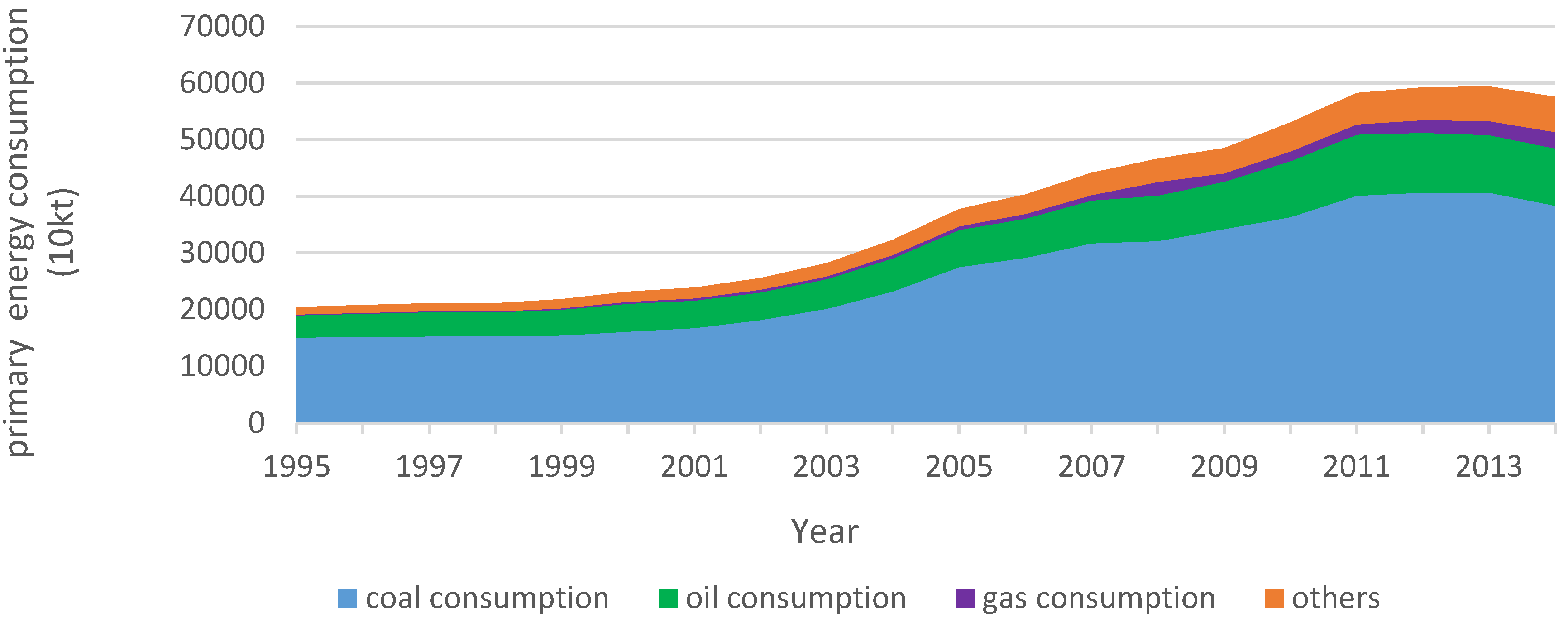
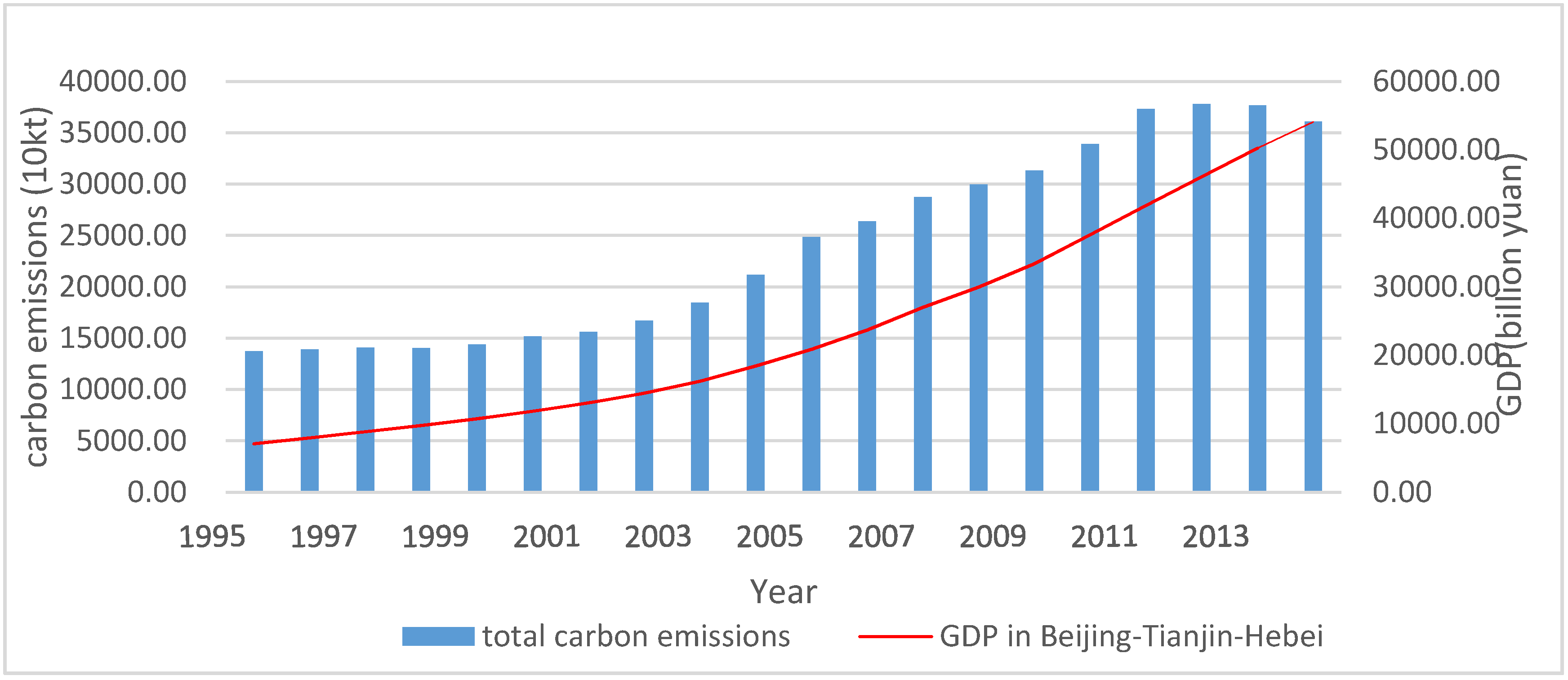
4.1. Evolution of Primary Energy Consumption, Carbon Emissions, and GDP

The total of the primary energy consumption in Beijing-Tianjin-Hebei region is shown in Figure 1. The amount of total energy consumption increased to 57,548.90 ktce in 2014 from 20,436.89 ktce in 1995, with a 9.08% annual increasing degree on average. Meanwhile, the coal consumption ratio in energy declined from 73.78% to 66.62% during the period of 1995–2014. On the whole, coal consumption had an absolute advantage, while the proportion of natural gas, oil and other energy sources were also increasing slowly in recent years, and the results demonstrate that the energy consumption structure will develop in the direction toward benign.

Figure source: The dates of primary energy consumption of various fossil energy types (1995–2014) were collected from the China Energy Statistical Yearbook, involving the energy consumption of raw coal, coke, crude oil, gasoline, kerosene, diesel oil, fuel oil, and gas.

The relationship between the carbon emissions of the energy consumption and economic growth is shown in Figure 2. From 1995 to 2014, the energy-related carbon emissions increased from 13,714.73 kt to 36,076.75 kt, with an average annual growth of 8.15%. During the same period, the average growth rate of economic growth and energy consumption were 33.44% and 8.40% respectively. Consequently, there was a strong correlation and synchronization between the economic growth and carbon emissions from energy consumption in Beijing-Tianjin-Hebei province.

Figure source: The GDP of Beijing, Tianjin, Hebei provinces were derived from the Beijing Statistical Yearbook, Tianjin Statistical Yearbook, and Hebei Economic Yearbook. Moreover, the GDP was be converted to 1995 price to eliminate inflation.

4.2. Generalized Fisher Index Results

Aiming to investigate the effective factors of carbon emissions from primary energy consumption in the Beijing-Tianjin-Hebei region, this study decomposed the influencing factors of carbon emissions into energy structure effect, energy intensity effect, economic output effect, and population scale effect. And we took 1995 as the base year and made yearly decompositions underlying the GFI model. The annual decomposition results and the contribution rate of influencing factors of carbon emissions are presented in

Table 3. Annual decomposition analysis results of changes in carbon emissions from energy consumption in the Beijing-Tianjin-Hebei region (1995–2014).

Time Interval	Energy Structure Effect	Energy Intensity Effect	Economic Output Effect	Population Scale Effect	Total Carbon Emissions Effect
1995–1996	0.9987	0.8981	1.1042	1.0176	1.0078
1996–1997	1.0038	0.8928	1.1145	1.0028	0.9963
1997–1998	1.0000	0.9271	1.0943	1.0064	1.0209
1998–1999	0.9966	0.9312	1.0897	1.0071	1.0185
1999–2000	0.9968	1.0139	1.0730	1.0286	1.1154
2000–2001	1.0011	0.9524	1.0952	1.0055	1.0500
2001–2002	1.0026	0.9633	1.0977	1.0085	1.0691
2002–2003	1.0015	0.9680	1.1119	1.0078	1.0864
2003–2004	1.0008	0.9881	1.1270	1.0097	1.1252
2004–2005	1.0025	0.9680	1.1206	1.0114	1.0997
2005–2006	0.9986	0.9617	1.1186	1.0151	1.0905
2006–2007	0.9994	0.9460	1.1193	1.0167	1.0760
2007–2008	0.9858	0.9317	1.0885	1.0208	1.0206
2008–2009	1.0098	0.9448	1.0938	1.0187	1.0631
2009–2010	0.9953	0.9695	1.0924	1.0329	1.0888
2010–2011	1.0009	0.9299	1.0994	1.0153	1.0389
2011–2012	0.9984	0.9427	1.0854	1.0147	1.0366
2012–2013	0.9998	0.9334	1.0765	1.0139	1.0185
2013–2014	0.9943	0.9354	1.0630	1.0122	1.0007
1995–2014	0.9813	0.3543	5.9105	1.3009	2.6733

and Figure 3.

Table source: Data interval covered 1995 to 2014. Energy structure $X_{2i}=E_i/E$ denotes the proportion of ith fossil energy in total energy consumption; Energy intensity $X_{3i}=E/Y$ refers to the energy consumption of per unit GDP; $X_{4i}=Y/P$ represents per capital of GDP; and $X_{5i}=P$ refers to population scale. The total population and GDP of the Beijing, Tianjin, Hebei provinces were derived from the Beijing Statistical Yearbook, Tianjin Statistical Yearbook, and Hebei Economic Yearbook. Moreover, the GDP was converted to 1995 price to eliminate inflation.

Figure source: The contribution rate of carbon emissions from energy consumption in Beijing-Tianjin-Hebei (1995–2014) were calculated using the GFI model.

4.2.1. Energy Structure Effect

The energy structure effect in the Beijing-Tianjin-Hebei region showed larger fluctuations during the period of 1995–2014. The cumulative energy structure effect of 1995 to 2014 was 0.9813, and the cumulative contribution rate was 12%. Overall, the larger fluctuation was divided into the stages of 1995–2005 and 2006–2014. At the first stage, energy structure effect values were all generally greater than 1, which denotes that energy structure effect is the main factor that promoted the increment of carbon emissions. Energy structure effect values were all generally smaller than 1 in the period of 2006–2014. Therefore, the inhibition of energy structure effect of carbon emissions from energy consumption became stronger in recent years. The results demonstrate that the predominance of energy consumption structure in Beijing-Tianjin-Hebei region was gradually optimized.

4.2.2. Energy Intensity Effect

The energy intensity effect was an important factor that restricts carbon emissions from energy consumption in the Beijing-Tianjin-Hebei region. The cumulative energy intensity effect of 1995 to 2014 was 0.3543, and the cumulative contribution rate was 4%. According to the yearly decomposition results, the energy intensity effect values were generally smaller than 1 from 1995 to 2014, which indicates that the energy intensity effect mainly inhibited carbon emissions from energy consumption. The energy intensity decreased from 2.7402 standard coal/million Yuan to 0.9709 standard coal/million Yuan, this shows that the technological progress and energy efficiency were significantly improved in Beijing-Tianjin-Hebei region. In other words, the decline of energy intensity denotes that the economy was developing rapidly in the Beijing-Tianjin-Hebei region, while the ratio of energy consumption was declining.

4.2.3. Economic Output Effect

The results of yearly decomposition show that economic output was a positive driving effect on carbon emissions from energy consumption, and it had a great contribution in this region from 1995 to 2014. The cumulative economic output effect of 1995 to 2014 was 5.9105, and the cumulative contribution rate was 69%, which was much larger than other factors and devotes the greatest contribution on carbon emission growth. Meanwhile, there were great differences in the extent of variation and change direction of carbon emissions during the three periods: 2001–2005, 2006–2008, and 2009–2014. During 2001–2005, the economic output of Beijing-Tianjin-Hebei region was on the rise, accordingly, the carbon emissions also increased. As a consequence of the arrival of twenty-first Century, Beijing-Tianjin-Hebei’s economy was in a period of vigorous development environment, thus the increment of carbon emissions was reasonable. During 2006–2008, the growth rate of economic output effect was gradually slowing down. On account of the Olympic Games in 2008, China adopted the energy conservation and other measures to protect the environment, accordingly, the energy consumption of the Beijing-Tianjin-Hebei region growth was limited. During 2009–2014, the region was affected by the financial crisis and the government’s policy of industrial structure adjustment, the economic output effect first rose and then declined.

4.2.4. Population Scale Effect

Population scale effect was another positive factor of carbon emissions in Beijing-Tianjin-Hebei region. The cumulative economic output effect of 1995 to 2014 was 1.3009, and the cumulative contribution rate was 15%. On the whole, the annual growth rate was relatively small, merely 1.47%. From 1995 to 2010, the population scale effect presented a rising trend, however, it began to decline year by year since 2011. The Beijing-Tianjin-Hebei region belongs to China’s important heavy industry and energy consumption areas, and the advantages of resources are more concentrated, especially, as the capital of China, Beijing attracts more and more talented people. Hebei is a province with a large population in China. The rigid demand for energy consumption contributes to the continuous increment of carbon emissions. From the overall development trend, the population scale effect of Beijing-Tianjin-Hebei region was enhancing year by year.

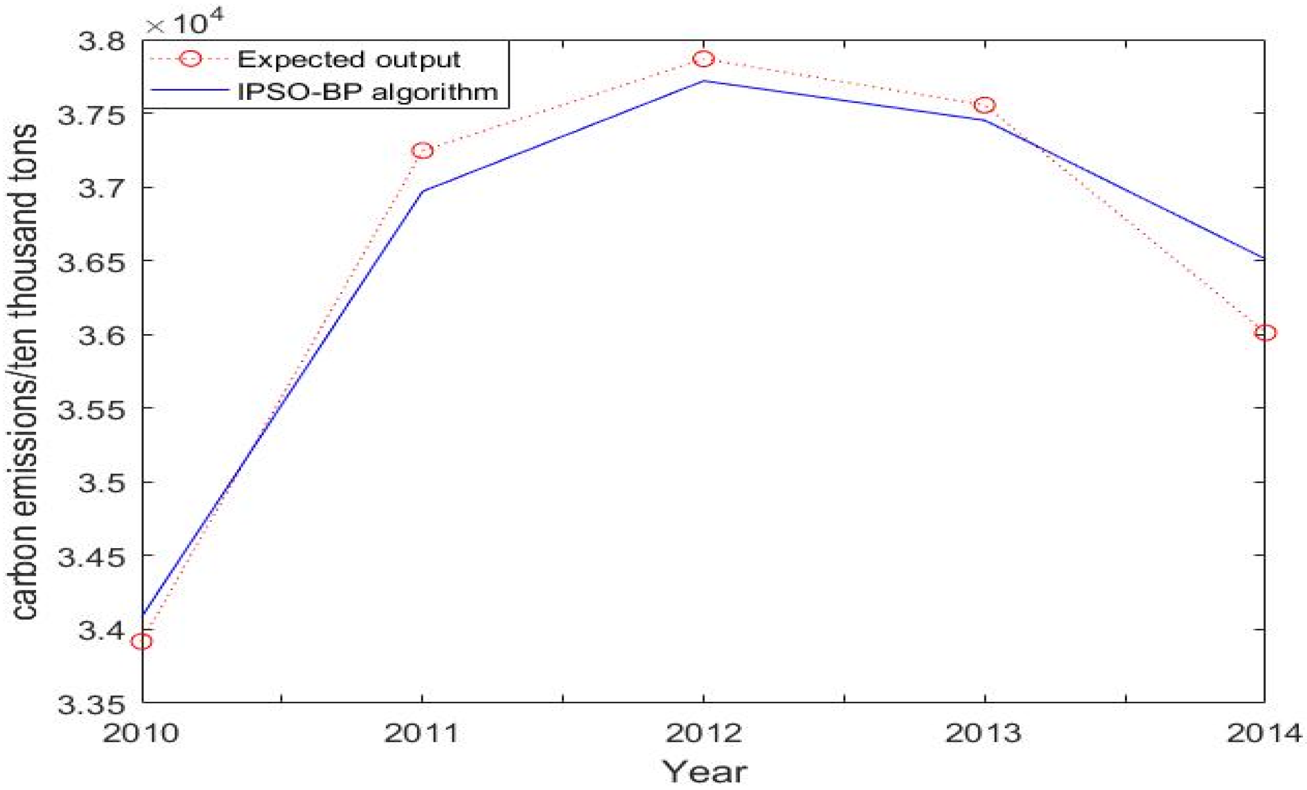
4.3. The Inspection Results of IPSO-BP Neural Network Model

Using the MATLAB (R2016a, MathWorks, Natick, MA, United States) programming language, this paper selected the data of carbon emissions from energy consumption in Beijing-Tianjin-Hebei region during the period of 1994–2009 as training samples, and used the remaining data during the period of 2010–2014 as testing samples. The aim was to train the IPSO-BP neural network and obtain the important parameters. The specific inspection results of this model are shown in Figure 4.

Figure source: This paper selected the data of carbon emissions from energy consumption in Beijing-Tianjin-Hebei region during the period of 1994–2009 as training samples, and the remaining data during the period of 2010–2014 as test samples, and obtained inspection results of the IPSO-BP neural network.

The IPSO-BP neural network can achieve the highest prediction accuracy through many training times when complying with the following conditions: The maximal algebra of network iteration is 140 times, meanwhile, the error precision and the learning rate are set to 0.0001 and 0.1, respectively. In the IPSO algorithm, the maximal algebra of iteration was 80 times, the number of population was 50, and the mutation probability was set to be 0.9; moreover, the search space was limited in [−3, 3], and velocity of swarm particles was in the interval [−1, 1]. The input indicators of this model were energy structure, energy intensity, economic output and population size, while the output indicator was carbon emissions from energy consumption in the Beijing-Tianjin-Hebei region. Under the above conditions, this paper employed the trained IPSO-BP neural network to predict the carbon emissions from energy consumption in the Beijing-Tianjin-Hebei region during 2010–2014, and through five training times, it obtained the average value. The results demonstrate that IPSO-BP neural network could better reflect the developing trend of carbon emissions during the time slot of 2010–2014. In predictive accuracy, the annual average relative error of IPSO-BP neural network was 2.53%, and it was believed that this model is well fitted to conduct the following study.

4.4. The Results of Scenario Prediction

4.4.1. Scenario Analysis Results for Influencing Factors

According to the decomposition results of carbon emissions from energy consumption in the Beijing-Tianjin-Hebei region, the main influencing factors were energy structure, energy intensity, economic output, and population scale. The decomposition results indicated that in the energy consumption structure, the proportion of coal consumption was the main proportion of energy consumption. Therefore, this paper employed the proportion of coal consumption instead of energy structure. The specific scenario prediction results of each influencing factors were as follows.

(1) The Scenario Analysis for Energy Structure

The result shows that the main source of the carbon emissions from energy consumption in Beijing-Tianjin-Hebei region was coal. Although the proportion of the oil and gas was slightly rising in recent years, the coal in energy consumption structure still accounted for a large proportion. Therefore, this paper employed the developing law of the proportion of the coal consumption in 2005–2014 to set the values in high carbon scenarios, and it could be obtained that the annual decline rate of coal consumption ratio was 0.86% during the period of 2015–2030 in high carbon scenario. According to the “energy development strategy action plan (2014–2020)”, China’s coal consumption ratio will be controlled within 62% by 2020. The national “12th Five-Year plan” clearly stated that non-fossil energy consumption accounted for 15% of total energy consumption by 2020. It can be obtained that the annual decline rate of coal consumption ratio was 0.99% in 2015–2030 in basic carbon scenario through calculation. In accordance with the experience of “China Energy Mid-and Long Term (2030, 2050) Development Strategy Research”, the annual decline rate of coal consumption ratio was 1.99% in low carbon scenario.

(2) The Scenario Analysis for Energy Intensity

On the basis of the decomposition results, the energy intensity effect was the main factor to inhibit the carbon emissions from energy consumption in Beijing-Tianjin-Hebei region. To ensure the objectivity of the high carbon scenario, this paper employed the developing law of energy intensity in 2005–2014 to set the values in high carbon scenarios, and it was obtained that the annual decline rate of energy intensity was 3.99%. According to the “2009 China sustainable development strategy report”, energy intensity will decrease by 40–60% in 2020. As the critical area of energy conserving and emission reduction, the Beijing-Tianjin-Hebei region is bound to accomplish these objectives. Therefore, this paper sets the decline rate of 60% as the basic scenario, and the decline rate of 65% as the low carbon scenario. Therefore, the annual decline rate of energy intensity in 2015–2030 under basic scenario and low carbon scenario will take the proportion of the value 4.77% and 5.96%, respectively.

(3) The Scenario Prediction for Population Scale

As the consequence of the “two-child policy” implemented widely in China in 2011, the growth rate of the population in the Beijing-Tianjin-Hebei region is likely to rise in recent years. Thus, this paper adopts the population development law of the past five years (2010–2014) to set the value of population scale in high carbon scenario, and it was obtained that the annual growth rate of population scale was 1.14% in 2015–2030. Based on the requirements of “Beijing 13th Five-Year Plan”, the total of resident population will reach approximately 1350 million in Beijing by the end of 2020. Similarly, in accordance with the “Tianjin 13th Five-Year Plan”, the total of residents population in Tianjin will be controlled within 18 million at the end of 2020. According to the “Hebei provincial population development strategy review meeting” in 2006, Hebei Province has entered the peak of the fourth birth population for more than ten years, and the total population will reach the peak around 2024, which is about 76.29 million. According to the above requirements, the annual population growth rate of Beijing, Tianjin, and Hebei in basic scenario were respectively designated as 0.98%, 2.67%, and 0.30% in 2015–2030. In compliance with the “the report on the population development strategy of Beijing, Tianjin and Hebei”, the total population will continue to maintain a slow growth trend by 2020. Moreover, restricted by the regional water resources, the Beijing-Tianjin-Hebei region has a reasonable population capacity of about 110 million. Therefore, in low carbon scenario, the annual population growth rate of Beijing-Tianjin-Hebei region can be set to 0.60% in 2015–2030.

(4) The Scenario Prediction for Economic Output

According to the results, the per capital GDP of Beijing-Tianjin-Hebei region was 36793.36 Yuan in 2014. The average annual growth rate of per capital GDP in Beijing-Tianjin-Hebei was 7.31% from 2010 to 2014. On the basis of the law of economic development in the developed countries, and accompanied with the rapid economic development, the trend tends of economic growth will be gentle. Consequently, it is reasonable to set the annual average growth rate in 2015–2020 and 2021–2030 as 7.31% and 6.81% in the high carbon scenario, respectively. In the basic scenario and the low carbon scenario, this paper firstly set the variation tendency of GDP. Then, the corresponding per capital GDP was calculated with the given data of population, according to the “Collaborative Development Planning of Beijing, Tianjin and Hebei Province” and the “13th Five-Year Plan” for the Beijing, Tianjin and Hebei province, which maintained an annual average growth rate of 6.5%, 8.5%, and 7% respectively in 2015–2020. In order to set the values of low carbon scenario, this study referred the scenario prediction for GDP put forward by reference [56], which believed that GDP will reduce by 0.5 percentage points per stage based on the basic scenario.

4.4.2. Scenario Prediction Results

In the light of the analysis and calculation, the specific scenario prediction values of four influencing factors was obtained during 2015–2030. Then, the well-trained IPSO-BP neural network model was applied to forecast the carbon emissions from energy consumption in the Beijing-Tianjin-Hebei region during 2015–2030 under the three different scenarios. Owing to the variation of the energy structure, energy intensity, economic output, and population scale, the total carbon emissions from energy consumption and the peak time were different under different scenarios. As shown in Figure 5, the predicted carbon emissions in high carbon scenario during 2015–2030 were the highest, followed by the basic scenario and low carbon scenario. In high carbon scenario, the carbon emissions will peak in 2028, which will be 40,280 million tons. In basic scenario, the carbon emissions will arrive at a peak around 2025 with 38,892 million tons, which was lower than the high carbon emissions. In low carbon scenario, the carbon emissions will have a decline stage between 2015 and 2018, with an annual decline rate of 0.38%, and then the carbon emissions will be in the ascending phase during 2019–2030. Furthermore, the peak of carbon emissions in the basic scenario will be three years ahead of the high carbon scenario and the peak value will also have a certain degree of reduction, which can reach 1388 million tons.

Figure source: Application of the well trained IPSO-BP neural network model to forecast the carbon emissions from energy consumption in the Beijing-Tianjin-Hebei region during 2015–2030 under three different scenarios, then obtaining the scenario prediction results of IPSO-BP neural network model.

5. Conclusions

In this study, the GFI model was utilized to delve into the influencing factors of carbon emissions from primary energy consumption, simultaneously, the IPSO-BP neural network and scenario prediction were exploited to analyze the carbon emissions from energy consumption in the Beijing-Tianjin-Hebei region under three scenarios during 2015–2030. The major conclusions are presented as follows:

(1)

Results reveal that energy consumption structure was developing toward benign direction in Beijing-Tianjin-Hebei region. Considering a strong correlation between the economic growth and carbon emissions from energy consumption, it is conducive to inhibit the increment of carbon emissions to some extent by reducing economic growth appropriately.

(2)

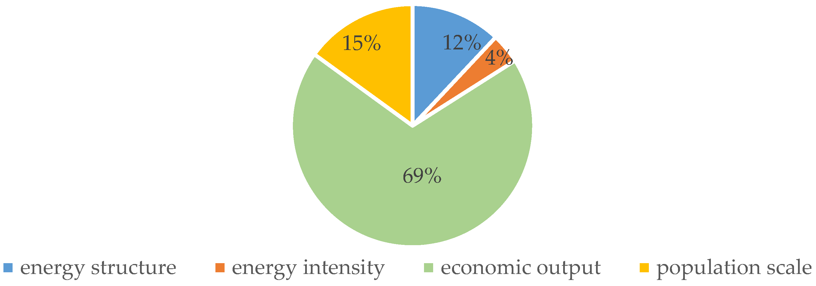
Over the study period, the effect of four driving factors on carbon emissions were different both in magnitude and in direction. The factors that drive the growth of carbon emissions from energy consumption in the Beijing-Tianjin-Hebei region were economic output and population scale, and the cumulative effect values were 5.9105 and 1.3009. Meanwhile, the contribution rates were 69% and 15%. On the contrary, the factors that mainly inhibited the carbon emissions were energy structure and energy intensity. The cumulative effect values were 0.3543 and 0.9813, and the contribution rates were 4% and 12%, respectively.

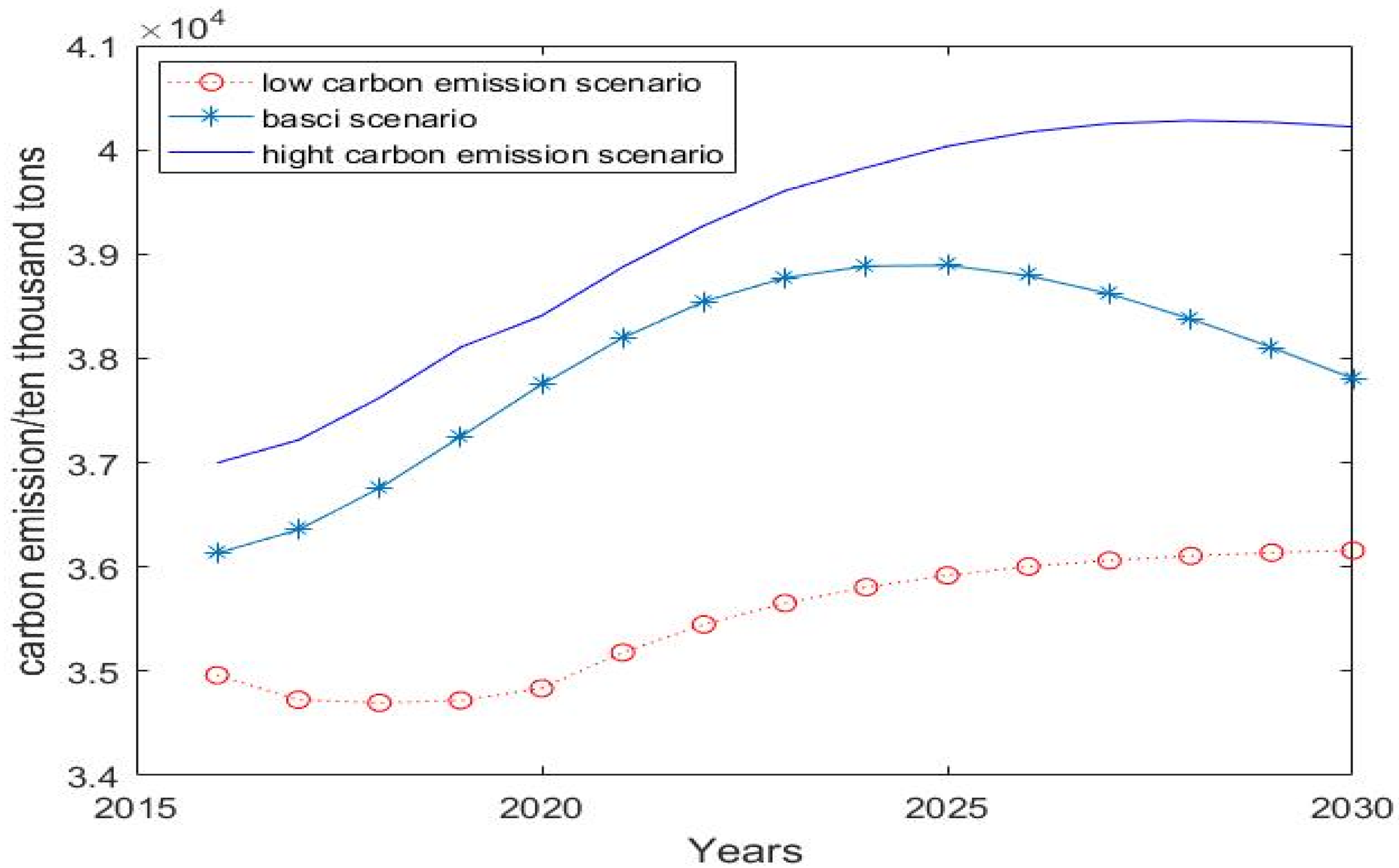
(3)

The predicted carbon emissions in high carbon scenario during 2015–2030 were the highest, followed by the basic scenario and low carbon scenarios. In the high carbon scenario, the carbon emissions will peak in 2028, which will be 40,280 million tons. In basic scenario, the carbon emissions will peak around 2025. In low carbon scenario, the carbon emissions will have a decline stage between 2015 and 2018, with an annual decline rate of 0.38%, and then the carbon emissions will be in the ascending phase during 2019–2030.

References

1. United Nations Framework Convention on Climate Change—The Paris Agreement. Available online: https://baike.sogou.com/v113787401.htm?fromTitle (accessed on 12 December 2015).
2. National Bureau of Statistics of the People’s Republic of China. Available online: http://www.stats.gov.cn/tjsj/ndsj/2017/indexch.htm (accessed on 13 October 2017).
3. Regional Planning for the Beijing-Tianjin-Hebei Metropolitan Area. Available online: https://baike.sogou.com/v71645024.htm (accessed on 5 August 2010).
4. National Development and Reform Commission (NDRC). Available online: http://www.ndrc.gov.cn/ (accessed on 8 December 2015).
5. The CPC Central Committee’s Proposal to Formulate the 11th Five-Year Plan for National Economic and Social Development. Available online: http://www.360doc.com/content/16/0308/21/19096873_540601354.shtml (accessed on 14 March 2006).
6. The CPC Central Committee’s Proposal to Formulate the 12th Five-Year Plan for National Economic and Social Development. Available online: http://news.hexun.com/2010/5yearplan/index.html (accessed on 18 May 2012).
7. Cheng, X.; Fan, L.; Wang, J. Can Energy Structure Optimization, Industrial Structure Changes, Technological Improvements, and Central and Local Governance Effectively Reduce Atmospheric Pollution in the Beijing-Tianjin-Hebei Area in China? Sustainability 2018, 10, 644. [Google Scholar] [CrossRef]
8. Wang, L.; Zhang, F.; Pilot, E.; Yu, J.; Nie, C.; Holdaway, J.; Yang, L.; Li, Y.; Wang, W.; Vardoulakis, S.; et al. Taking Action on Air Pollution Control in the Beijing-Tianjin-Hebei (BTH) Region: Progress, Challenges and Opportunities. Int. J. Environ. Res. Public Health 2018, 15, 306. [Google Scholar] [CrossRef] [PubMed]
9. Cai, B.; Li, W.; Dhakal, S.; Wang, J. Source data supported high resolution carbon emissions inventory for urban areas of the Beijing-Tianjin-Hebei region: Spatial patterns, decomposition and policy implications. J. Environ. Manag. 2018, 206, 786–799. [Google Scholar] [CrossRef] [PubMed]
10. Li, J. Scenario analysis of tourism’s water footprint for China’s Beijing-Tianjin-Hebei region in 2020: Implications for water policy. J. Sustain. Tour. 2018, 26, 127–145. [Google Scholar] [CrossRef]
11. Li, J.; Xiang, Y.; Jia, H.; Chen, L. Analysis of Total Factor Energy Efficiency and Its Influencing Factors on Key Energy-Intensive Industries in the Beijing-Tianjin-Hebei Region. Sustainability 2018, 10, 111. [Google Scholar] [CrossRef]
12. Qi, J.; Zheng, B.; Li, M.; Yu, F.; Chen, C.; Liu, F.; Zhou, X.; Yuan, J.; Zhang, Q.; He, K. A high-resolution air pollutants emission inventory in 2013 for the Beijing-Tianjin-Hebei region, China. Atmos. Environ. 2017, 170, 156–168. [Google Scholar] [CrossRef]
13. Can, W.; Jining, C.; Ji, Z. Decomposition of energy-related CO2 emission in China: 1957–2000. Energy 2005, 30, 73–83. [Google Scholar]
14. Salim, R.; Yao, Y.; Chen, G.; Zhang, L. Can foreign direct investment harness energy consumption in China? A time series investigation. Energy Econ. 2017, 66, 43–53. [Google Scholar] [CrossRef]
15. Yan, Q.; Yin, J.; Baležentis, T.; Makutėnienė, D.; Štreimikienė, D. Energy-related GHG emission in agriculture of the European countries: An application of the Generalized Divisia Index. J. Clean. Prod. 2017, 164, 686–694. [Google Scholar] [CrossRef]
16. Zhou, X.; Zhang, J.; Li, J. Industrial structural transformation and carbon dioxide emissions in China. Energy Policy 2013, 57, 43–51. [Google Scholar] [CrossRef]
17. Bhattacharya, M.; Paramati, S.R.; Ozturk, I.; Bhattacharya, S. The effect of renewable energy consumption on economic growth: Evidence from top 38 countries. Appl. Energy 2016, 162, 733–741. [Google Scholar] [CrossRef]
18. Zhang, L. Correcting the uneven burden sharing of emission reduction across provinces in China. Energy Econ. 2017, 64, 335–345. [Google Scholar] [CrossRef]
19. Chen, J.D.; Cheng, S.L.; Nikic, V.; Songm, M.L. Quo Vadis? Major Players in Global Coal Consumption and Emissions Reduction. Transform. Bus. Econ. 2018, 17, 112–132. [Google Scholar]
20. Sheinbaum, C.; Ruíz, B.J.; Ozawa, L. Energy consumption and related CO2 emissions in five Latin American countries: Changes from 1990 to 2006 and perspectives. Energy 2011, 36, 3629–3638. [Google Scholar] [CrossRef]
21. Lin, B.; Du, K. Decomposing energy intensity change: A combination of index decomposition analysis and production-theoretical decomposition analysis. Appl. Energy 2014, 129, 158–165. [Google Scholar] [CrossRef]
22. Hatzigeorgiou, E.; Polatidis, H.; Haralambopoulos, D. CO2 emissions in Greece for 1990–2002: A decomposition analysis and comparison of results using the Arithmetic Mean Divisia Index and Logarithmic Mean Divisia Index techniques. Energy 2008, 33, 492–499. [Google Scholar] [CrossRef]
23. Ang, B.W. Decomposition analysis for policymaking in energy: Which is the preferred method? Energy Policy 2004, 32, 1131–1139. [Google Scholar] [CrossRef]
24. Akpan, U.S.; Green, O.A.; Bhattacharyya, S.; Isihak, S. Effect of Technology Change on CO2 Emissions in Japan’s Industrial Sectors in the Period 1995–2005: An Input-Output Structural Decomposition Analysis. Environ. Resour. Econ. 2015, 61, 165–189. [Google Scholar] [CrossRef]
25. Croner, D.; Frankovic, I. A Structural Decomposition Analysis of Global and National Energy Intensity Trends. Energy J. 2018, 39, 103–122. [Google Scholar]
26. Su, B.; Ang, B.W. Multi-region comparisons of emission performance: The structural decomposition analysis approach. Ecol. Ind. 2016, 67, 78–87. [Google Scholar] [CrossRef]
27. Su, B.; Ang, B.W. Attribution of changes in the generalized Fisher index with application to embodied emission studies. Energy 2014, 69, 778–786. [Google Scholar] [CrossRef]
28. Wang, H.; Ang, B.W.; Su, B. Multiplicative structural decomposition analysis of energy and emission intensities: Some methodological issues. Energy 2017, 123, 47–63. [Google Scholar] [CrossRef]
29. Cansino, J.M.; Román, R.; Ordóñez, M. Main drivers of changes in CO2 emissions in the Spanish economy: A structural decomposition analysis. Energy Policy 2016, 89, 150–159. [Google Scholar] [CrossRef]
30. Koppány, K. Estimating growth contributions by structural decomposition of input-output tables. Acta Oecon. 2018, 67, 605–642. [Google Scholar] [CrossRef]
31. Román-Collado, R.; Colinet, M.J. Is energy efficiency a driver or an inhibitor of energy consumption changes in Spain? Two decomposition approaches. Energy Policy 2018, 115, 409–417. [Google Scholar] [CrossRef]
32. Jimenez, R.; Mercado, J. Energy intensity: A decomposition and counterfactual exercise for Latin American countries. Energy Econ. 2014, 42, 161–174. [Google Scholar] [CrossRef]
33. Xu, X.Y.; Ang, B.W. Multilevel index decomposition analysis: Approaches and application. Energy Econ. 2014, 44, 375–382. [Google Scholar] [CrossRef]
34. Kaivo-oja, J.; Luukkanen, J.; Panula-Ontto, J.; Vehmas, J.; Chen, Y.; Mikkonen, S.; Auffermann, B. Are structural change and modernisation leading to convergence in the CO2 economy? Decomposition analysis of China, EU and USA. Energy 2014, 72, 115–125. [Google Scholar] [CrossRef]
35. Román, R.; Cansino, J.M.; Rodas, J.A. Analysis of the main drivers of CO2 emissions changes in Colombia (1990–2012) and its political implications. Renew. Energy 2018, 116, 402–411. [Google Scholar] [CrossRef]
36. Winyuchakrit, P.; Limmeechokchai, B. Trends of energy intensity and CO2 emissions in the Thai industrial sector: The decomposition analysis. Energy Sources Part B Econ. Plan. Policy 2016, 11, 504–510. [Google Scholar] [CrossRef]
37. Chen, B.; Li, J.S.; Zhou, S.L.; Yang, Q.; Chen, G.Q. GHG emissions embodied in Macao’s internal energy consumption and external trade: Driving forces via decomposition analysis. Renew. Sustain. Energy Rev. 2018, 82, 4100–4106. [Google Scholar] [CrossRef]
38. Torrie, R.D.; Stone, C.; Layzell, D.B. Understanding energy systems change in Canada: 1. Decomposition of total energy intensity. Energy Econ. 2016, 56, 101–106. [Google Scholar] [CrossRef]
39. Xu, J.H.; Fleiter, T.; Eichhammer, W.; Fan, Y. Energy consumption and CO2 emissions in China’s cement industry: A perspective from LMDI decomposition analysis. Energy Policy 2012, 50, 821–832. [Google Scholar] [CrossRef]
40. Xu, S.C.; He, Z.X.; Long, R.Y. Factors that influence carbon emissions due to energy consumption in China: Decomposition analysis using LMDI. Appl. Energy 2014, 127, 182–193. [Google Scholar] [CrossRef]
41. Fang, D.; Zhang, X.; Yu, Q.; Jin, T.C.; Tian, L. A novel method for carbon dioxide emission forecasting based on improved Gaussian processes regression. J. Clean. Prod. 2018, 173, 143–150. [Google Scholar] [CrossRef]
42. Sun, W.; Xu, Y. Using a back propagation neural network based on improved particle swarm optimization to study the influential factors of carbon dioxide emissions in Hebei Province, China. J. Clean. Prod. 2016, 112, 1282–1291. [Google Scholar] [CrossRef]
43. Marjanović, V.; Milovančević, M.; Mladenović, I. Prediction of GDP growth rate based on carbon dioxide (CO2) emissions. J. CO2 Utilizat. 2016, 16, 212–217. [Google Scholar] [CrossRef]
44. Ito, K. CO2 emissions, renewable and non-renewable energy consumption, and economic growth: Evidence from panel data for developing countries. Int. Econ. 2017, 151, 1–6. [Google Scholar] [CrossRef]
45. Zoundi, Z. CO2 emissions, renewable energy and the Environmental Kuznets Curve, a panel cointegration approach. Renew. Sustain. Energy Rev. 2017, 72, 1067–1075. [Google Scholar] [CrossRef]
46. Mrabet, Z.; Alsamara, M. Testing the Kuznets Curve hypothesis for Qatar: A comparison between carbon dioxide and ecological footprint. Renew. Sustain. Energy Rev. 2017, 70, 1366–1375. [Google Scholar] [CrossRef]
47. Deviren, S.A.; Deviren, B. The relationship between carbon dioxide emission and economic growth: Hierarchical structure methods. Physica A 2016, 451, 429–439. [Google Scholar] [CrossRef]
48. Mladenović, I.; Sokolov-Mladenović, S.; Milovančević, M.; Marković, D.; Simeunović, N. Management and estimation of thermal comfort, carbon dioxide emission and economic growth by support vector machine. Renew. Sustain. Energy Rev. 2016, 64, 466–476. [Google Scholar] [CrossRef]
49. De Boer, P. Generalized Fisher index or Siegel–Shapley decomposition? Energy Econ. 2009, 31, 810–814. [Google Scholar] [CrossRef]
50. Ang, B.W.; Liu, F.L.; Chung, H.S. A generalized Fisher index approach to energy decomposition analysis. Energy Econ. 2004, 26, 757–763. [Google Scholar] [CrossRef]
51. IPCC (Intergovernmental Panel on Climate Change). 2006 IPCC Guidelines for National Greenhouse Gas Inventories; Eggleston, H.S., Buendia, L., Miwa, K., Ngara, T., Tanabe, K., Eds.; Prepared by the National Greenhouse Gas Inventories Programme; IGES: Hayama, Japan, 2006. [Google Scholar]
52. Kaya, Y. Impact of Carbon Dioxide Emission Control on GNP Growth: Interpretation of Proposed Scenarios; Paper presented at the IPCC Energy and Industry Subgroup; Response Strategies Working Group: Paris, France, 1990. [Google Scholar]
53. FallahHoseini, M.; Rafeh, R. Proposing a centralized algorithm to minimize message broadcasting energy in wireless sensor networks using directional antennas. Appl. Soft Comput. 2018, 64, 272–281. [Google Scholar] [CrossRef]
54. Vinita, J.; Punam, B. An improved hybrid ant particle optimization (IHAPO) algorithm for reducing travel time in VANETs. Appl. Soft Comput. 2018, 64, 526–535. [Google Scholar]
55. Yin, Y.; Mizokami, S.; Aikawa, K. Compact development and energy consumption: Scenario analysis of urban structures based on behavior simulation. Appl. Energy 2015, 159, 449–457. [Google Scholar] [CrossRef]
56. Wen, L.; Liu, Y. The Peak Value of Carbon Emissions in the Beijing-Tianjin-Hebei Region Based on the STIRPAT Model and Scenario Design. Pol. J. Environ. Stud. 2016, 25, 823–834. [Google Scholar] [Green Version]
Figure 1. The total of primary energy consumption in the Beijing-Tianjin-Hebei region from 1995 to 2014.
Energies 11 01489 g001
Figure 2. The relationship between the total carbon emissions and GDP in the Beijing-Tianjin-Hebei region from 1995 to 2014.
Energies 11 01489 g002
Figure 3. The influencing factors of carbon emissions from primary energy consumption in Beijing-Tianjin-Hebei (1995–2014).
Energies 11 01489 g003
Figure 4. The result of CO2 emission of expect output and the inspection results of the improved particle swarm optimization-back propagation (IPSO-BP) neural network during the period of 2010–2014.
Energies 11 01489 g004
Figure 5. The results of the CO2 emission predicted by IPSO-BP neural network model in the Beijing-Tianjin-Hebei region at three different scenarios during 2015–2030.
Energies 11 01489 g005