Impacts of the Allocation Mechanism Under the Third Phase of the European Emission Trading Scheme


Abstract
1. Introduction
- The move to a single Union-wide cap instead of national caps standardised the approach to improve the harmonisation of ambition between Member States and therefore the level of allocation to their industries.
- Auctioning has become the default method for allowance distribution, reducing the number of allowances that are provided for free. Theoretically auctioning of allowances is preferred since it avoids rent seeking behavior in decision about distribution of allocations. Further, auctioning is consistent with the polluter pays principle which likely increases the perceived fairness of the auction’s outcome [2]. However, in practice auctioning shares so far remained low except in the electricity sector because of concerns over carbon leakage. Free allocation is considered as second best to protect leakage exposed industries [4].
- Harmonised rules for free allocation based on benchmarks (for products and fall-back approaches for heat and fuels) standardised the approach for installations within each sector or subsector. The product benchmarks have been defined based on the 10% best performing installations. The benchmark-based allocation rewards efficient installations that will receive a relatively complete endowment with certificates to cover their emissions while installations with a relatively poor emission performance will face a deficit in allocations compared to emissions.
- How do allocations compare with actual installation verified emissions? The purpose of this analysis is to determine at detailed sector and country level, the evolution from Phase I/II (which have been characterised by large over-allocation) to Phase III.
- How do actual verified emissions of installations compare with benchmark values? For that purpose, we focus in an exemplary manner on four important products: cement clinker, pig iron production, ammonia production and the production of nitric acid (as an important emitter of nitrous oxide N2O, a powerful greenhouse gas).
2. Methodology and Data
2.1. Methodology for the Comparison of Allocation with Actual Emissions
- In a first step, the ratio of allocation to verified emissions was established for 2008, as a year of the second trading period that was probably not yet affected by the economic downturn, as well as for 2013 as the starting year for the 3rd trading period. The year 2013 was used to focus the analysis on effects from the introduction of benchmark-based allocation. Otherwise, the linear reduction of allocation to installations producing non-carbon leakage exposed products would also be captured. The two ratios indicate whether there had been surpluses in allocation.
- Second, the ratio of allocation 2008 to verified emissions 2008 was calculated as an indicator for potential over-allocation of free allowances at the start of the 2nd trading period.
- Third, the ratio of allocation 2013 to average allocation 2nd trading period was calculated. Substracting one from this ratio gives the percentage change in allocation.
2.2. Methodology for Measuring Impacts of Benchmarks for Allocation on Verified Emissions
- First, a subset of installation data concerning emissions is selected from the public European Transaction Log EUTL [19] for the sector which covers the whole period from 2005 up to the last available year in the register at the time of the analysis (2017, i.e., the fifth year in Phase III). Limitations in the availability of production data limited this, however, de facto to 2016, except for pig iron. Data for plants which have been closed or opened in the period of consideration were excluded from the dataset. For nitric acid and ammonia, this approach was not possible, as these products entered the ETS only in 2013; hence, in difference to cement clinker and pig iron, the EUTL does not contain data from 2005 to 2012 and analysis before Phase III had to be taken interviews with the association Fertilizers Europe [23].
- Second, the activity data for the different products and individual installations available for the period 2005–2010 were taken from a non-public database collected for the allocation for Phase III of the ETS, the so-called National Implementation Measures (NIMS) data. Production was available in an aggregate manner for each product considered in this paper but with the same underlying disaggregation of installations as for the emissions. Below we will discuss the importance of having the same installations for emissions and activities. Mostly this information is for the period 2005–2008. The activity measure is the same activity measure used for the benchmarks [3], i.e., usually physical production of the product group.
- As installations can be fairly heterogeneous entities, the installations had to be decomposed into sub-installations, where each sub-installation reflected as close as possible the definition of the processes underlying the benchmark definition of interest. The NIMS data mentioned above, further provide information on the share of an installation’s allocation at sub-installation level for product and fallback benchmarks. This was also based on average shares for the period 2005–2010. The assumption is made that the emissions shares for the product benchmarks for different sub-installations in overall emissions of the installation remain the same over time as the split indicated for the period 2005–2010. For cement clinker these average shares are 98% and for pig iron 79%. The emissions of the installations are then corrected with these factors to extract the emissions relevant for the product benchmark under consideration. This was only possible for cement clinker and pig iron, as ammonia and nitric acid were not part of the EUTL before 2013 (or only with production parts such as steam generators).
- The activities are then extended to 2016/2017—the last year for which data on emissions for installations or production data are available—by use of an index. This avoids the problem that the ratio of emissions and activity data is impacted by a different delimitation of numerator and denominator, at least to a large degree as the indices are less influenced than the absolute levels.
- Such indices can be derived in principle from the following data sources:
- ○
- Prodcom statistics (based on total production volume) [24]
- ○
- Activity statistics from associations
We discuss in the following the quality of these sources. In particular, Prodcom data may have problems with respect to the completeness of data. - The emission data corrected for the shares of the product benchmarks are then divided by the extrapolated activity data and compared with the benchmarks to calculate which emission reduction may have occurred. If an installation produces several products the share of each product would be considered separately with this approach to allow a comparison of emissions compared to the benchmark. The emission parts allocated to the fall back sub-installations are excluded from the consideration. However, for cement clinker and pig iron the share of the main sub-installation considered here is very large compared to other product groups.
3. Results
3.1. Comparison of Allocation with Actual Emissions
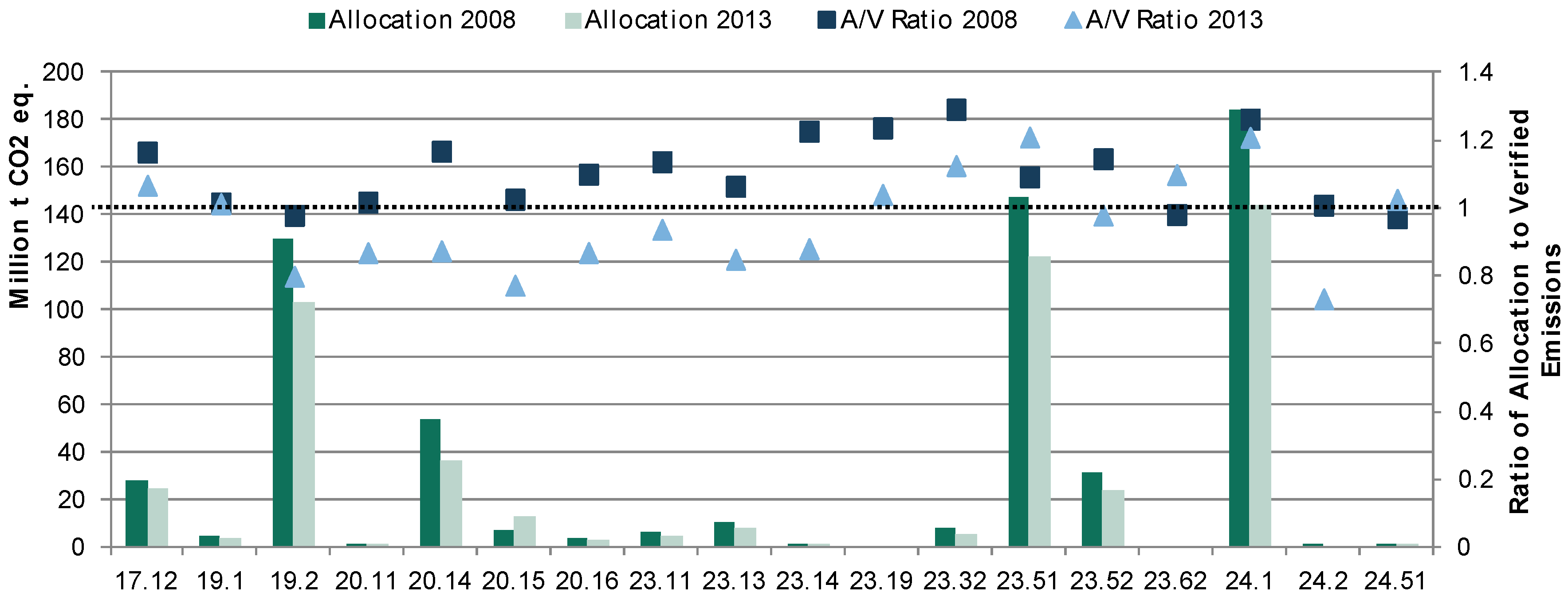
3.1.1. Allocation Changes at Sectoral Level
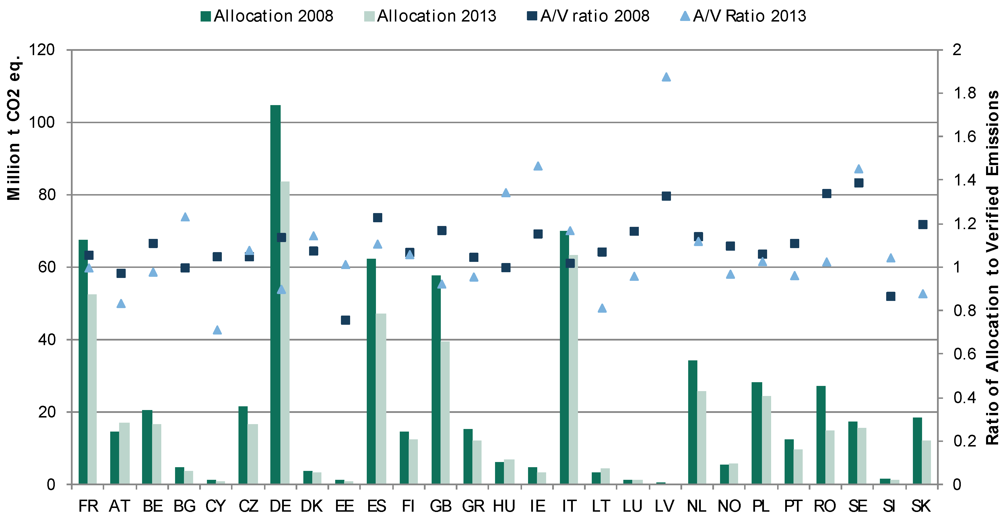
3.1.2. Allocation Changes at Country Level
3.1.3. Allocation Changes and Verified Emissions for Country-Sector Pairs
3.2. Impact of Benchmarks for Allocation on Verified Emissions
3.2.1. Cement
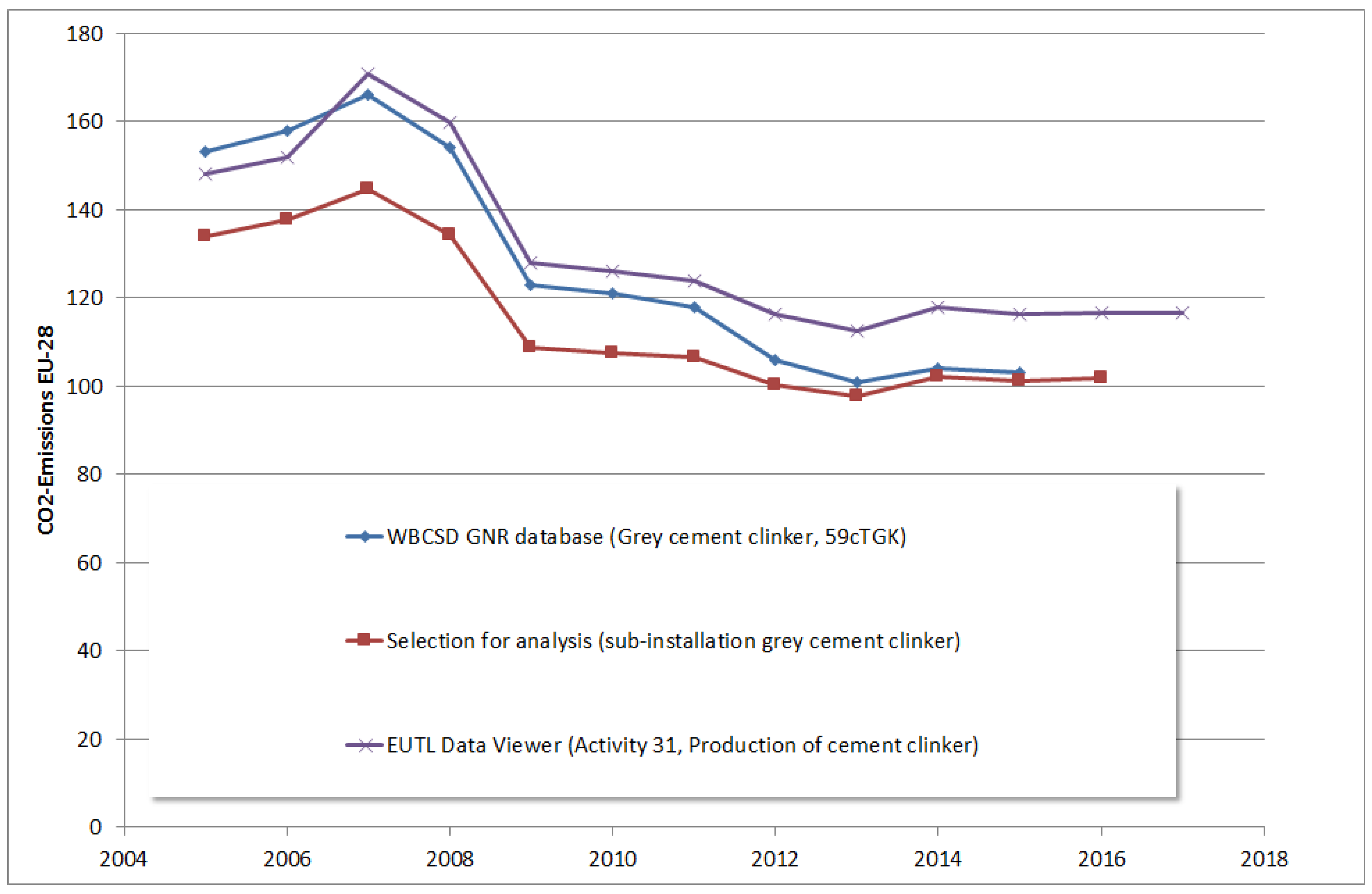
- data from the EUTL data viewer [25] (activity 29, production of cement clinker);
- data from the GNR database run by the World Business Council for Sustainable Development WBCSD [26];
- data prepared for our case study based on the EUTL registers [19]. This concerned a selection of installations which had a continued production in the period 2005–2016 (i.e., plants which were only producing part of the period were taken out from the analysis. The dataset was corrected for the effect that the verified emissions also contain partly emissions from other sub-installations than cement clinker. This data set is rather close to the verified emissions of the selected data set as cement clinker sub-installations represent the overwhelming parts of the verified emissions of the installations. The correction was made based on the share of the clinker sub-installations in the period 2005–2010 (as obtained from NIMS data).
- Coverage of installations: We identified 241 installations in the EU EUTL as cement clinker plants. The emissions of the selection of installations are shown in Figure 5. This curve follows the trend in the EUTL data viewer rather parallel. The emissions from the 241 plants do not show the strong decrease in emissions as evident from the GNR data from 2011 onwards. It was emphasised by Cembureau that the coverage of cement installations in the GNR database fell from 98% of the total in 2011 to 95% in 2013, which contributes to the observed difference in verified emissions. However, it may possibly not impact much on specific emissions as a change in coverage would impact both on emissions and on production. If a production index is derived from the GNR database for clinker and used in combination with the emission data derived from the register, the specific emissions would increase in 2012–2013, given the change in coverage in production (derived from GNR) but not impacting also on the emissions (derived from the registers). Finally, several EUTL installations were removed by Cembureau on the grounds that the installations were not correctly classified under EUTL activity code and may in fact contain emissions from other processes (i.e., lime production).
- Changes in reporting protocol: Cembureau confirmed that part of the decline in emissions after 2012 in the GNR database is due to a change in accounting rules for emissions from waste. The change in methodology for emission factors has been operated actually to improve the comparability between the EUTL and GNR datasets as the GNR dataset was previously more stringent in accounting for waste emissions than the EUTL (according to the previous methodology, emissions from tire combustion were considered as originating from fossil fuels and taken fully into account by GNR. However about one quarter is biomass-based and considered as CO2-free in the new methodology). The change was introduced, starting in 2012. However, not all companies have been reporting immediately according to the new methodology. It is likely that 2012 and 2013 (perhaps also still 2014) is a mixture of reporting according to old and new methodology. It is clear that this change in accounting rules lowers the emissions starting 2012, as compared to the previous years.
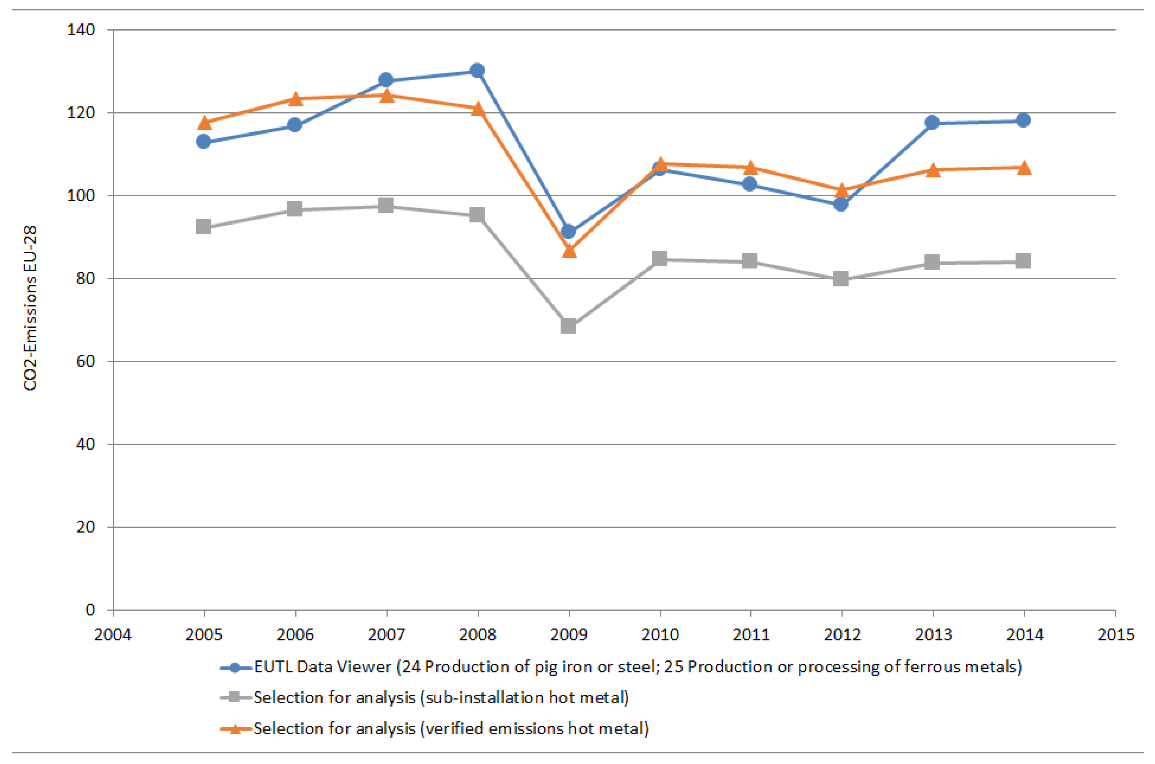
3.2.2. Pig Iron Production (Molten Metal)
- Differences in the volume of molten metal and pig iron, which was used here, as a proxy: However, the differences are not important.
- A variety of installations are registered in an emission “bubble” which also includes other installations in an integrated steel mill. However, this would have as a result rather higher emissions compared to the benchmark.
- The most important point is, however, that waste gases arising from blast furnaces and steel converter are also exported to generate electricity, i.e., either within the integrated steel mill and hence possibly within the associated emission bubble. Or the export goes to another site. The issue is then how these emissions are accounted for between the provider of the waste gas and the electricity generators and how the associated allowances are distributed between user and provider of the waste gas. Though normally electricity generation is not receiving allowances for free, waste gases receive nevertheless allowances up to the level which makes them comparable with natural gas for electricity generation. For blast furnace gas, this is roughly three quarters of the emissions from that type of gas. If the allowances for this are largely given to the user, then the specific emissions of molten metal appear as lower than the benchmark. This arrives with a variety of installations.
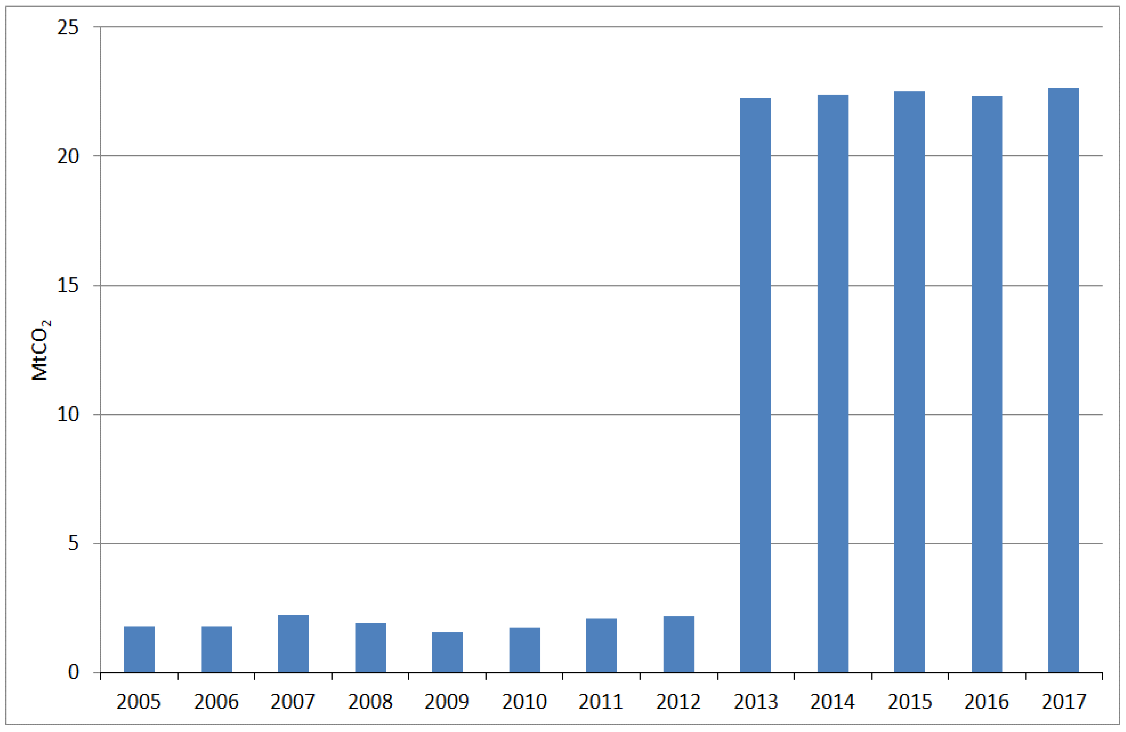
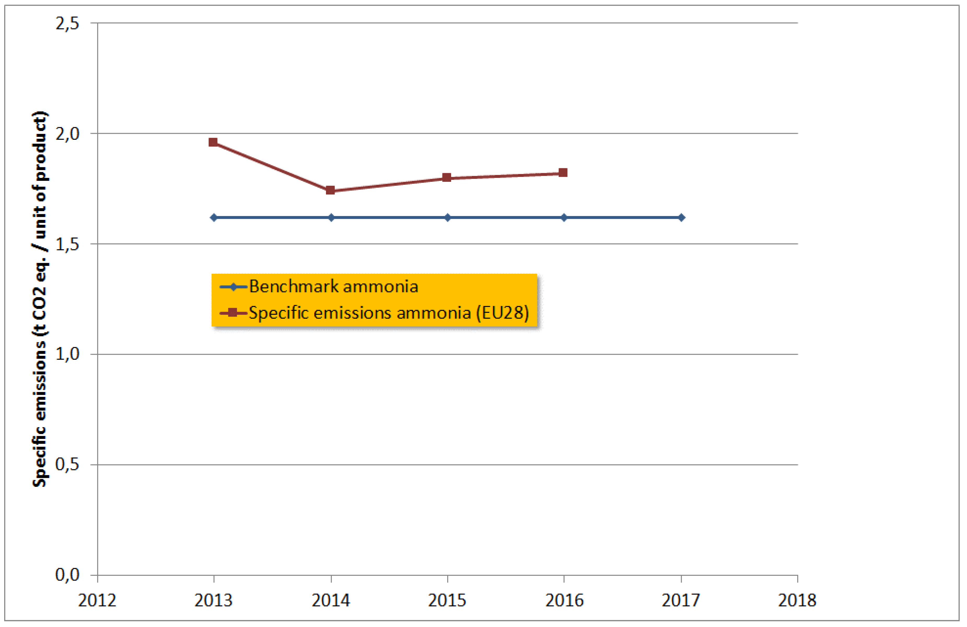
3.2.3. Ammonia
- The 2007–2008 average net energy efficiency of 35.2 GJ/mt NH3 was a 1.3% improvement over the previous period. This improvement is primarily a result of better efficiency performance by the same plants. Additional three new plants had a neutral impact on the average.
- The 2010–2011 average net energy efficiency of 34.9 GJ/mt NH3 was a 0.8% improvement over the previous period.
- The 2013–2014 average net energy efficiency of 34.8 GJ/mt NH3 was a 0.2% improvement over the previous period.
3.2.4. Nitric Acid
4. Discussion
4.1. Discussion of Results for the Comparison of Allocation with Actual Emissions
- Allocation changes at sectoral: At the aggregate level, i.e., comparing the sum of allocations 2008–2013 per sector, allocation decreased in all but two sectors. On average the changed allocation contributed to the reduction of a surplus in allocations compared to verified emissions. While the ratio of allocation to verified emissions was larger than 1 in all but three sectors, the ratio was smaller than one in all but six sectors in 2013. For three sectors, in particular cement, the allocation to verified emissions ratio is larger in 2013 than in 2008 (see discussion below).
- Allocation changes at country level: In 2008, in 23 out of 27 countries allocation exceeded verified emissions. Even though allocations decreased in most countries, still in more than half of the countries, allocations exceed verified emissions in 2013. However, changes are quite disperse within the countries in particular driven by the heterogeneity of changes observed at sectoral level.
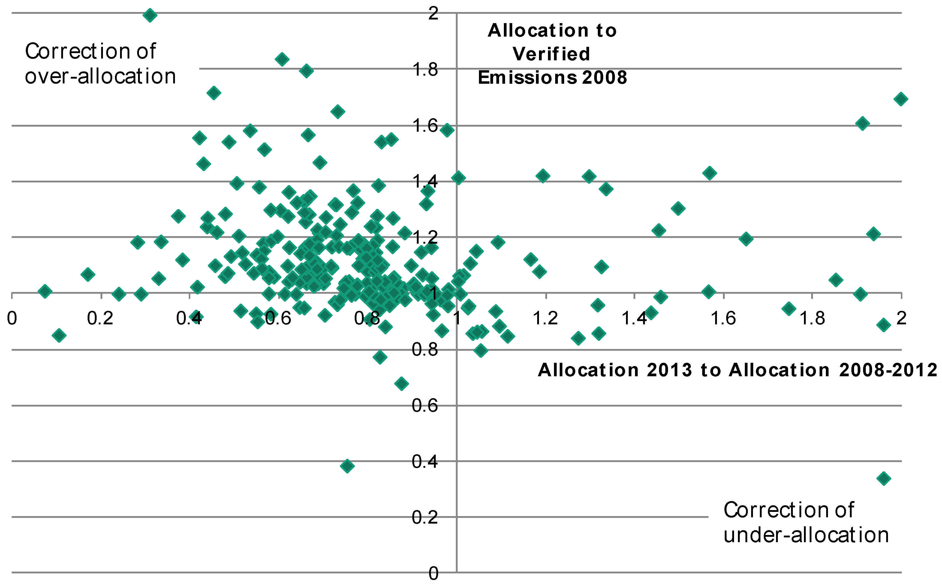
- Allocation changes and verified emissions for country-sector pairs: Looking at the heterogeneity of the allocation changes, the subsequent question is whether the changes contributed to reducing allocation surpluses that existed in 2008 and achieved a more harmonized allocation. The analysis of allocation/verified emission ratios for country-sector pairs shows that for the majority of country sector pairs, the ratio of Allocation 2013 to Average 2nd trading period was smaller than one while the ratio of allocations to verified emission in 2008 was larger than one. This can be interpreted as a correction of a potential historical over-allocation with the new allocation rules for the third trading period. The findings indicate that the benchmark-based allocation contributed to harmonizing allocation by reducing allocation more strongly for installations which have been over-allocated in the past.
- Cement: Previous analysis has found that for the cement sector installation emissions in 2012 clustered around capacity thresholds [30]. This indicates that installations’ operators reduced production and strategically exploited the rules for capacity changes to optimize their allocation situation. This effect contributes to explaining that despite decreased allocation, the cement sector has a higher allocation surplus over verified emissions in 2013 than in 2008. Notably, this is likely not related to improvements in operational efficiency. On the contrary, operating several plants at reduced capacity instead of closing one and operating the other at full capacity leads to decreased efficiency. Furthermore, the ambition to retain certain clinker production levels to meet the threshold may have led to increase clinker ratios in cement production.
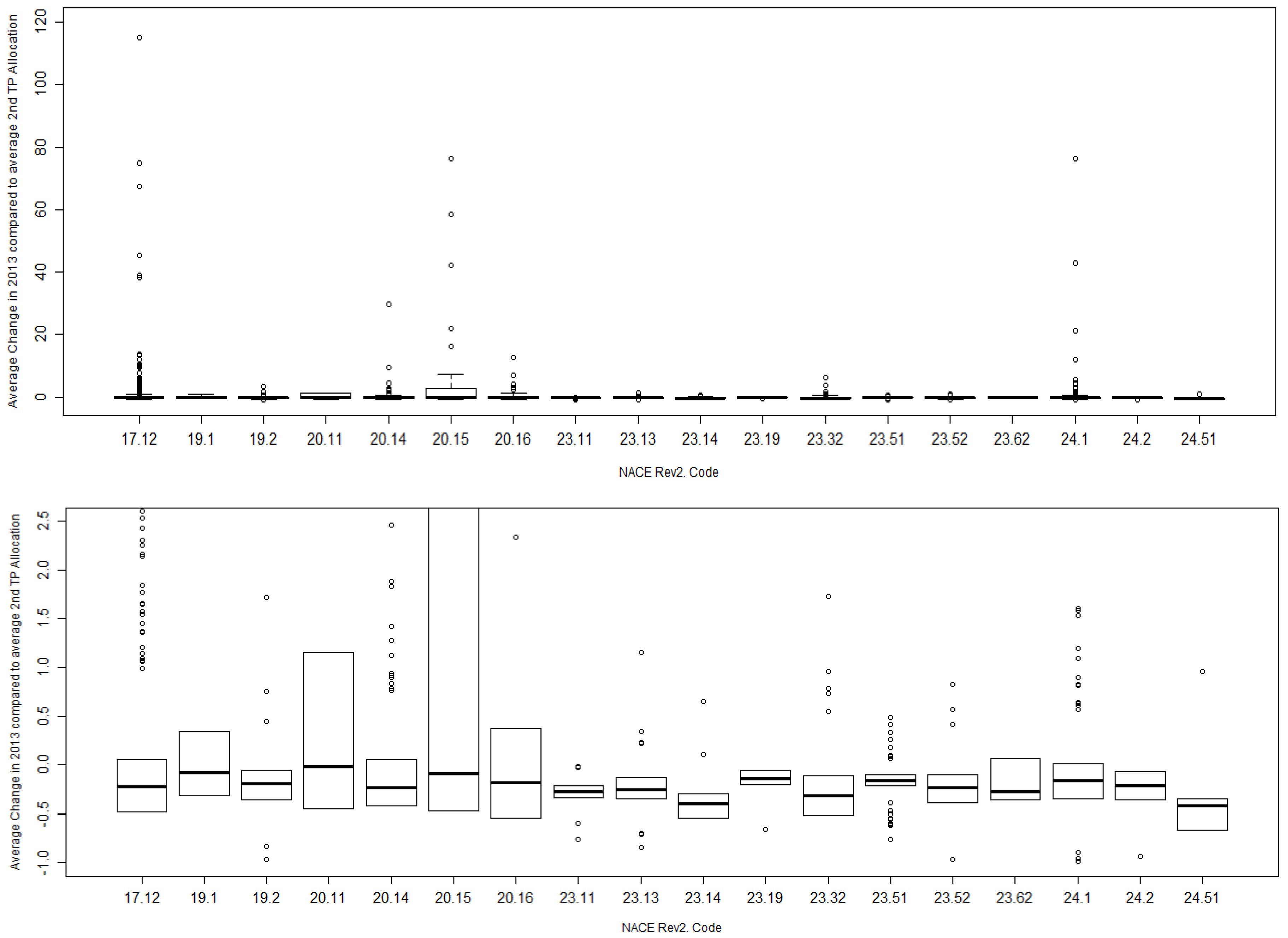
- Fertilisers and nitrogen compounds: The allocation increase in 2013 compared to 2008 at sector level for 20.15 Manufacture of fertilisers and nitrogen compounds (20.15) and 20.11 is driven by very high allocation changes in some installations. The median shows that most of the installations considered faced a decrease in allocation even though lower than in the other sectors. The installations with the largest allocation rise also had substantial changes in verified emissions from 2008 to 2013 which most likely relates to the changed scope of the EU ETS in its third trading period: Installations from the fertilizer sector only entered the EU ETS in 2013, but some installations have been liable to emissions trading before as thermal installations with a rated capacity of above 20 MW. Due to the low number of observations in the fertilizer sector particular effects from single installations have a stronger impact on the overall sector results.
- Pulp/paper: The treatment of cross-boundary heat flows probably strongly affected allocation in the paper sector in which combined heat and power installations are very common. For the paper sector in the Scandinavian countries numerous installations received an increased allocation in 2013 compared to the 2nd trading period even though allocations exceeded verified emissions in 2008. There are two explanatory factors: (a) Scandinavian paper mills are often integrated mills using a high share of biomass inputs and waste from the pulping process. Those mills are better off compared to stand-alone paper production under benchmark based allocation; (b) under allocation based on historical emissions, these installations will have had relatively low allocations compared to mills using less biomass and/or stand-alone mill because they have fewer emissions.
4.2. Discussion of Results for the Impacts of Benchmarks for Allocation on Verified Emissions
5. Conclusions and Outlook
Author Contributions
Acknowledgments
Conflicts of Interest
References
- Del Río González, P. Harmonization versus decentralization in the EU ETS: An economic analysis. Clim. Policy 2006, 6, 457–475. [Google Scholar] [CrossRef]
- Betz, R.; Rogge, K.; Schleich, J. EU emissions trading: An early analysis of national allocation plans for 2008–2012. Clim. Policy 2006, 6, 361–394. [Google Scholar] [CrossRef]
- European Commission. Commission Decision of 27 April 2011 determining transitional Union-wide rules for harmonised free allocation of emission allowances pursuant to Article 10a of Directive 2003/87/EC of the European Parliament and of the Council. Off. J. Eur. Union 2011, L130, 1–45. [Google Scholar]
- Sartor, O.; Pallière, C.; Lecourt, S. Benchmark-based allocations in EU ETS Phase 3: An early assessment. Clim. Policy 2014, 14, 507–524. [Google Scholar] [CrossRef]
- Ellerman, A.D.; Convery, F.J.; de Perthuis, C. Pricing Carbon: The European Union Emissions Trading Scheme; Cambridge University Press: Cambridge, UK, 2010; ISBN 978-05-21-19647-5. [Google Scholar]
- Ellermann, A.D.; Mercantonini, A.; Zaklan, A. The European Union Emissions Trading System: Ten Years and Counting. Rev. Environ. Econ. Policy 2010, 10, 89–107. [Google Scholar] [CrossRef]
- Muûls, M.; Colmer, J.; Martin, R.; Wagner, U.J. Evaluating the EU Emissions Trading System: Take It or Leave It? An Assessment of the Data after Ten Years. Grantham Institute Briefing Paper No. 21. Imperial College London. October 2016. Available online: https://www.imperial.ac.uk/media/imperial-college/grantham-institute/public/publications/briefing-papers/Evaluating-the-EU-emissions-trading-system_Grantham-BP-21_web.pdf (accessed on 31 May 2018).
- Fallmann, H.; Heller, C.; Seuss, K.; Voogt, M.; Phylipsen, D.; van Iersel, S.; Oudenes, M.; Zelljadt, E.; Tröltzsch, J.; Duwe, M.; et al. Evaluation of the EU ETS Directive; Publications Office of the European Union: Luxembourg, 2016; ISBN 978-92-79-55340-0. Available online: https://publications.europa.eu/en/publication-detail/-/publication/0478baf0-d6d4-11e5-8fea-01aa75ed71a1/language-en (accessed on 31 May 2018).
- Sato, L.; Laing, T.; Cooper, S.; Wang, L. Methods for Evaluating the Performance of Emissions Trading Schemes. Climate Strategies Discussion Paper. November 2015. Available online: https://climatestrategies.org/wp-content/uploads/2015/11/CS-ChinaETS-Evaluation-paper-final1.pdf (accessed on 31 May 2018).
- Umweltbundesamt. Evaluierung und Weiterentwicklung des EU-Emissionshandels. Climate Change 16/2016. Umweltbundesamt: Berlin, Germany. Available online: https://www.umweltbundesamt.de/sites/default/files/medien/378/publikationen/climate_change_16_2016_evaluierung_und_weiterentwicklung_des_eu-emissionshandels.pdf (accessed on 31 May 2018). (In German).
- Healy, S.; Schumacher, K.; Eichhammer, W. Analysis of Carbon Leakage under Phase III of the EU Emissions Trading System: Trading Patterns in the Cement and Aluminium Sectors. Energies 2018, 11, 1231. [Google Scholar] [CrossRef]
- Nils, A.; Oberndorfer, U. Firm Performance and Employment in the EU Emissions Trading Scheme: An Empirical Assessment for Germany. Energy Policy 2008, 36, 12–22. [Google Scholar] [CrossRef]
- Rogge, K. Reviewing the Evidence on the Innovation Impact of the EU Emission Trading System. SSRN Electron. J. 2016. [Google Scholar] [CrossRef]
- Finance for Innovation: Towards the ETS Innovation Fund. Available online: https://ec.europa.eu/clima/events/articles/0115_en (accessed on 2 May 2018).
- Betz, R.A.; Schmidt, T.S. Transfer patterns in Phase I of the EU Emissions Trading System: A first reality check based on cluster analysis. Clim. Policy 2015, 16, 474–495. [Google Scholar] [CrossRef]
- Duscha, V.; del Rio, P. An economic analysis of the interactions between renewable support and other climate and energy policies. Energy Environ. 2016, 28, 11–33. [Google Scholar] [CrossRef]
- Schlomann, B.; Eichhammer, W. Interaction between Climate, Emissions Trading and Energy Efficiency Targets. Energy Environ. 2014, 25, 709–731. [Google Scholar] [CrossRef]
- Heindl, P. The impact of administrative transaction costs in the EU emissions trading system. Clim. Policy 2015, 17, 314–329. [Google Scholar] [CrossRef]
- European Union Transaction Log (EUTL). Available online: http://ec.europa.eu/environment/ets/welcome.do (accessed on 2 May 2018).
- NACE Rev. 2—Statistical Classification of Economic Activities. Available online: http://ec.europa.eu/eurostat/web/products-manuals-and-guidelines/-/KS-RA-07-015 (accessed on 2 May 2018).
- European Commission. Commission Decision of 27 October 2014 determining, pursuant to Directive 2003/87/EC of the European Parliament and of the Council, a list of sectors and subsectors which are deemed to be exposed to a significant risk of carbon leakage, for the period 2015 to 2019. Off. J. Eur. Union 2014, L308/114, 114–124. [Google Scholar]
- Reuter, M.; Eichhammer, W. Applying ex-post index decomposition analysis to final energy consumption for evaluating European energy efficiency policies and targets. Energy Effic. 2018. under review. [Google Scholar]
- Fertilizers Europe (Auderghem, Belgium). Phillip Townsend Associates PTAI on behalf of Fertilizer Europe. Personal communication, 2016. [Google Scholar]
- Prodcom—Statistics by Product. Excel Files (NACE Rev.2), Various Years. Available online: http://ec.europa.eu/eurostat/web/prodcom/data/excel-files-nace-rev.2 (accessed on 2 May 2018).
- EU Emissions Trading System (ETS) Data Viewer. Available online: https://www.eea.europa.eu/data-and-maps/dashboards/emissions-trading-viewer-1 (accessed on 2 May 2018).
- Global Cement Database on CO2 and Energy Information. “Getting the Numbers Right” (GNR) Atabase. World Business Council for Sustainable Development WBCSD. Available online: http://www.wbcsdcement.org/index.php/key-issues/climate-protection/gnr-database (accessed on 2 May 2018).
- World Steel Association. Steel Statistical Yearbook 2017. Available online: https://www.worldsteel.org/en/dam/jcr:3e275c73-6f11-4e7f-a5d8-23d9bc5c508f/Steel+Statistical+Yearbook+2017.pdf and previous years (accessed on 2 May 2018).
- Arens, M.; Worrell, E.; Eichhammer, W. Drivers and barriers to the diffusion of energy-efficient technologies—A plant-level analysis of the German steel industry. Energy Effic. 2017, 2, 441–457. [Google Scholar] [CrossRef]
- Anderson, B.; Di Maria, C. Abatement and Allocation in the Pilot Phase of the EU ETS. Environ. Resour. Econ. 2011, 48, 83–103. [Google Scholar] [CrossRef]
- Climate Strategies. Carbon Control and Competitiveness Post 2020: The Cement Report. Final Report. February 2014. Available online: http://climatestrategies.org/wp-content/uploads/2014/02/climate-strategies-cement-report-final.pdf (accessed on 2 May 2018).


| NACE Rev. 2 | Subsector Name | Number of Installations in Sample | Average Allocation 2008–2012 (Mt CO2eq) | Allocation 2013 (Mt CO2eq) | Allocation Change 2013 Compared to Average 2nd TP |
|---|---|---|---|---|---|
| 17.12 | paper and paperboard | 493 | 30.14 | 24.24 | −20% |
| 19.1 | coke oven products | 17 | 4.93 | 4.11 | −17% |
| 19.2 | refined petroleum products | 112 | 133.49 | 102.90 | −23% |
| 20.11 | industrial gases | 5 | 1.26 | 1.40 | 11% |
| 20.14 | other organic basic chemical | 147 | 55.23 | 35.92 | −35% |
| 20.15 | fertilisers and nitrogen compounds | 46 | 8.17 | 13.00 | 59% |
| 20.16 | plastics in primary forms | 47 | 3.43 | 2.84 | −17% |
| 23.11 | flat glass | 42 | 6.04 | 4.20 | −31% |
| 23.13 | hollow glass | 167 | 10.98 | 7.86 | −28% |
| 23.14 | glass fibres | 44 | 1.44 | 0.89 | −38% |
| 23.19 | other glass, incl. technical glassware | 35 | 0.79 | 0.62 | −22% |
| 23.32 | bricks, tiles, construction products, in baked clay | 360 | 8.04 | 5.12 | −36% |
| 23.51 | cement | 198 | 149.25 | 122.29 | −18% |
| 23.52 | lime and plaster | 184 | 32.11 | 23.94 | −25% |
| 23.62 | plaster products for construction purposes | 7 | 0.20 | 0.17 | −15% |
| 24.1 | basic iron and steel and of ferro-alloys | 226 | 184.88 | 144.00 | −22% |
| 24.2 | tubes, pipes, hollow profiles and related fittings, of steel | 11 | 1.01 | 0.64 | −36% |
| 24.51 | casting of iron | 9 | 1.54 | 0.89 | −43% |
| Total | 2150 | 632.94 | 495.01 | −22% |
| Registry Code/Country | Number of Installations in Sample | Average Allocation 2008–2012 (Mt CO2eq) | Allocation 2013 (Mt CO2eq) | Allocation Change 2013 Compared to Average 2nd TP |
|---|---|---|---|---|
| AT-Austria | 70 | 14.72 | 16.87 | 15% |
| BE-Belgium | 91 | 21.01 | 16.67 | −21% |
| BG-Bulgaria | 19 | 4.89 | 3.65 | −25% |
| CY-Cyprus | 1 | 1.34 | 0.84 | −37% |
| CZ-Czech Republic | 87 | 20.74 | 16.78 | −19% |
| DE-Germany | 435 | 107.70 | 83.68 | −22% |
| DK-Denmark | 26 | 3.87 | 3.33 | −14% |
| EE-Estonia | 7 | 1.15 | 1.06 | −8% |
| ES-Spain | 221 | 64.56 | 47.11 | −27% |
| FI-Finland | 40 | 14.58 | 12.50 | −14% |
| FR-France | 233 | 68.47 | 52.38 | −23% |
| GB-Great Britain | 118 | 58.42 | 39.33 | −33% |
| GR-Greece | 43 | 15.23 | 11.94 | −22% |
| HU-Hungary | 33 | 6.03 | 7.01 | 16% |
| IE-Ireland | 10 | 4.74 | 3.32 | −30% |
| IT-Italy | 283 | 70.50 | 63.39 | −10% |
| LT-Latvia | 11 | 3.72 | 4.33 | 16% |
| LU-Luxembourg | 5 | 1.20 | 1.09 | −10% |
| LV-Latvia | 6 | 0.53 | 0.19 | −64% |
| NL-Netherlands | 75 | 36.27 | 25.84 | −29% |
| NO-Norway | 27 | 5.80 | 5.63 | −3% |
| PL-Poland | 87 | 29.26 | 24.44 | −16% |
| PT-Portugal | 55 | 12.78 | 9.65 | −24% |
| RO-Romania | 53 | 28.28 | 14.81 | −48% |
| SE-Sweden | 71 | 17.71 | 15.66 | −12% |
| SI-Slovenia | 18 | 1.50 | 1.29 | −14% |
| SK-Slovak Republic | 25 | 17.94 | 12.21 | −32% |
| Total | 2150 | 632.94 | 495.01 | −22% |
| NACE Rev. 2 | Number of Installations | Quantiles | |||||
|---|---|---|---|---|---|---|---|
| x.0% | x.25% | x.50% | x.75% | x.100% | |||
| 17.12 | paper and paperboard | 493 | −98% | −48% | −22% | 5% | 175,330% |
| 19.1 | coke oven products | 17 | −40% | −32% | −8% | 34% | 98% |
| 19.2 | refined petroleum products | 112 | −96% | −36% | −20% | −6% | 334% |
| 20.11 | industrial gases | 5 | −83% | −45% | −2% | 115% | 129% |
| 20.14 | other organic basic chemical | 147 | −98% | −42% | −24% | 5% | 2976% |
| 20.15 | fertilisers/nitrogen compounds | 46 | −93% | −46% | −9% | 256% | 7628% |
| 20.16 | plastics in primary forms | 47 | −86% | −55% | −18% | 37% | 1281% |
| 23.11 | flat glass | 42 | −76% | −33% | −28% | −22% | −2% |
| 23.13 | hollow glass | 167 | −84% | −35% | −26% | −13% | 115% |
| 23.14 | glass fibres | 44 | −84% | −55% | −40% | −30% | 65% |
| 23.19 | other glass, including technical glassware | 35 | −66% | −21% | −15% | −6% | 16% |
| 23.32 | bricks, tiles and construction products, in baked clay | 360 | −98% | −51% | −31% | −11% | 610% |
| 23.51 | cement | 198 | −76% | −22% | −16% | −10% | 49% |
| 23.52 | lime and plaster | 184 | −96% | −39% | −24% | −10% | 82% |
| 23.62 | plaster products for construction purposes | 7 | −42% | −36% | −28% | 7% | 22% |
| 24.1 | basic iron/steel; ferro−alloys | 226 | −99% | −35% | −16% | 2% | 7621% |
| 24.2 | tubes, pipes, hollow profiles and related fittings, of steel | 11 | −94% | −36% | −22% | −7% | 29% |
| 24.51 | Casting of iron | 9 | −90% | −67% | −42% | −34% | 96% |
| Product | Observation |
|---|---|
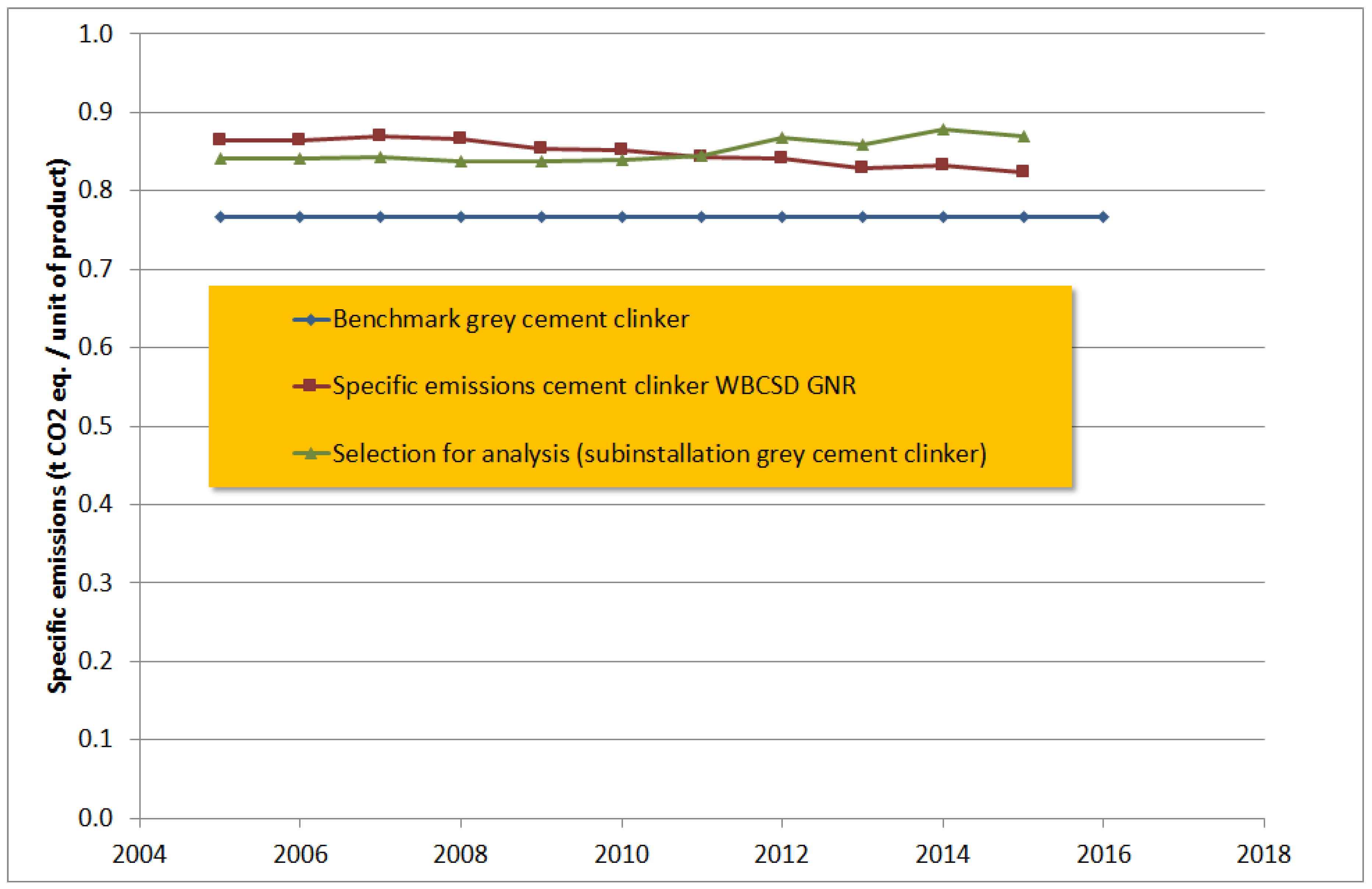
| Cement clinker | Specific emissions have been fairly stable between 2005 and 2011 and were consistently above the benchmark value. Our results show an increase in specific emissions between 2011 and 2013, which imply that the benchmarking rules have so far not encouraged a decline in the specific emissions of cement clinker plants in Europe. It is possible that the specific emissions of several cement clinker plants may have increased due to lower rates of capacity utilisation and a temporary increase in the ratio of clinker used in cement due to declining domestic demand following the economic recession. |
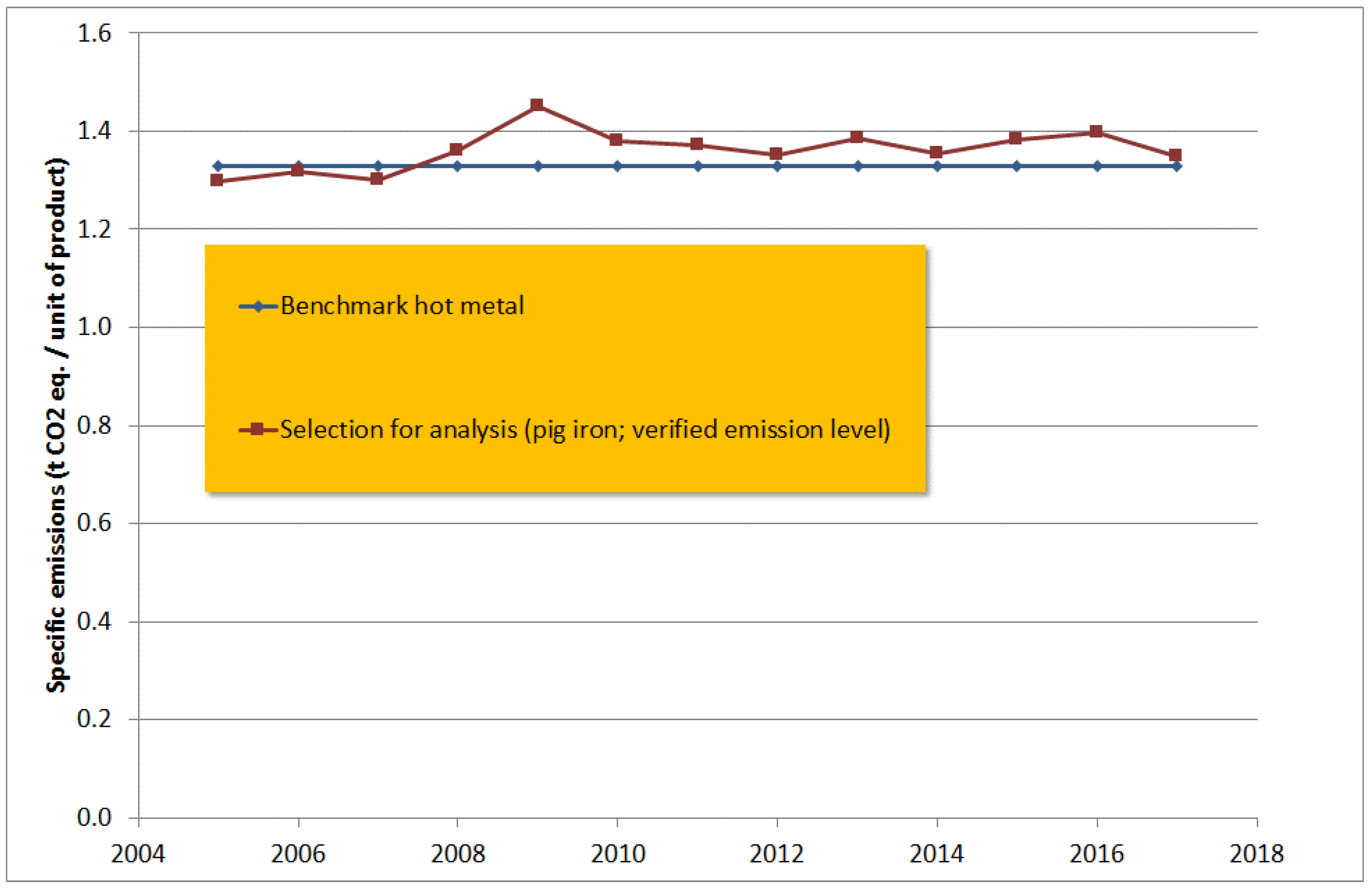
| Pig iron | The relative change of the specific emissions over time is small, suggesting—except for the period of the economic crisis in 2009, which has led to a rather low capacity use—no indication of low carbon technology being implemented to a substantial degree. Our specific emission calculation provide an absolute level below the hot metal benchmark: the reason is that emissions and allowances can be shared among producers and users of blast furnace gases for electricity generation. Though normally electricity generation is not receiving allowances for free, waste gases receive nevertheless allowances up to the level which makes them comparable with natural gas for electricity generation (For blast furnace gas roughly three quarters of the emissions). If the allowances for this are largely given to the user, then the specific emissions of molten metal appear as lower than the benchmark. This arrives with a variety of installations. |
| Ammonia | Energy efficiency improved through three surveys carried out by Fertilizer Europe by around 2.3% in 9 years, or about 0.25% per year in the period 2004–2013 (mostly in Eastern Member States where the processes were still more inefficient and the change brought economic benefits given increasing prices for natural gas) The ETS would have had a minor role, especially as ammonia only entered the ETS formally in 2013. However, the perspective of the ETS could have spurred the uptake of new technology. The analysis provided for the period 2013–2016 shows a rather flat evolution of specific emissions from ammonia appears. |
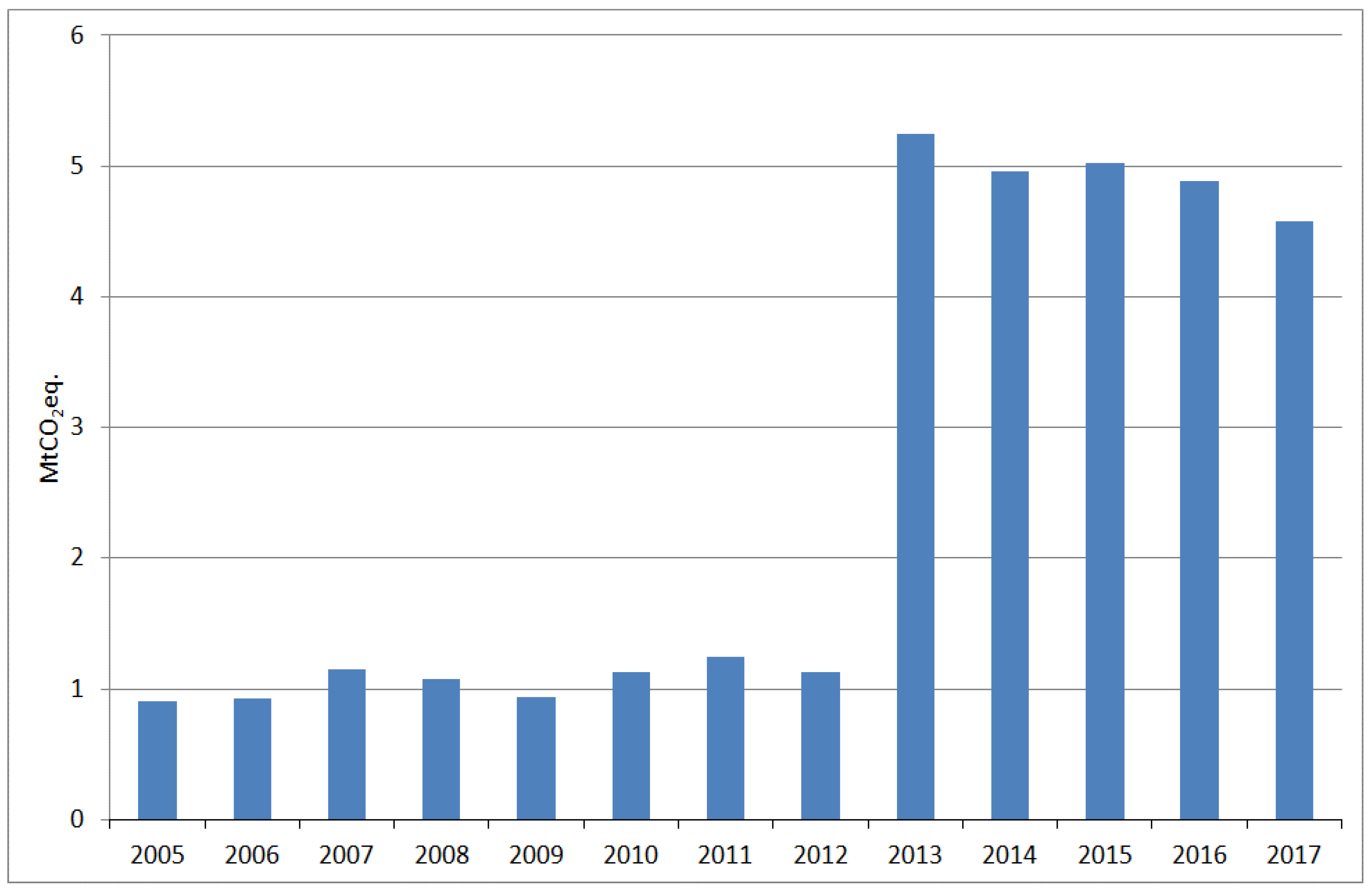
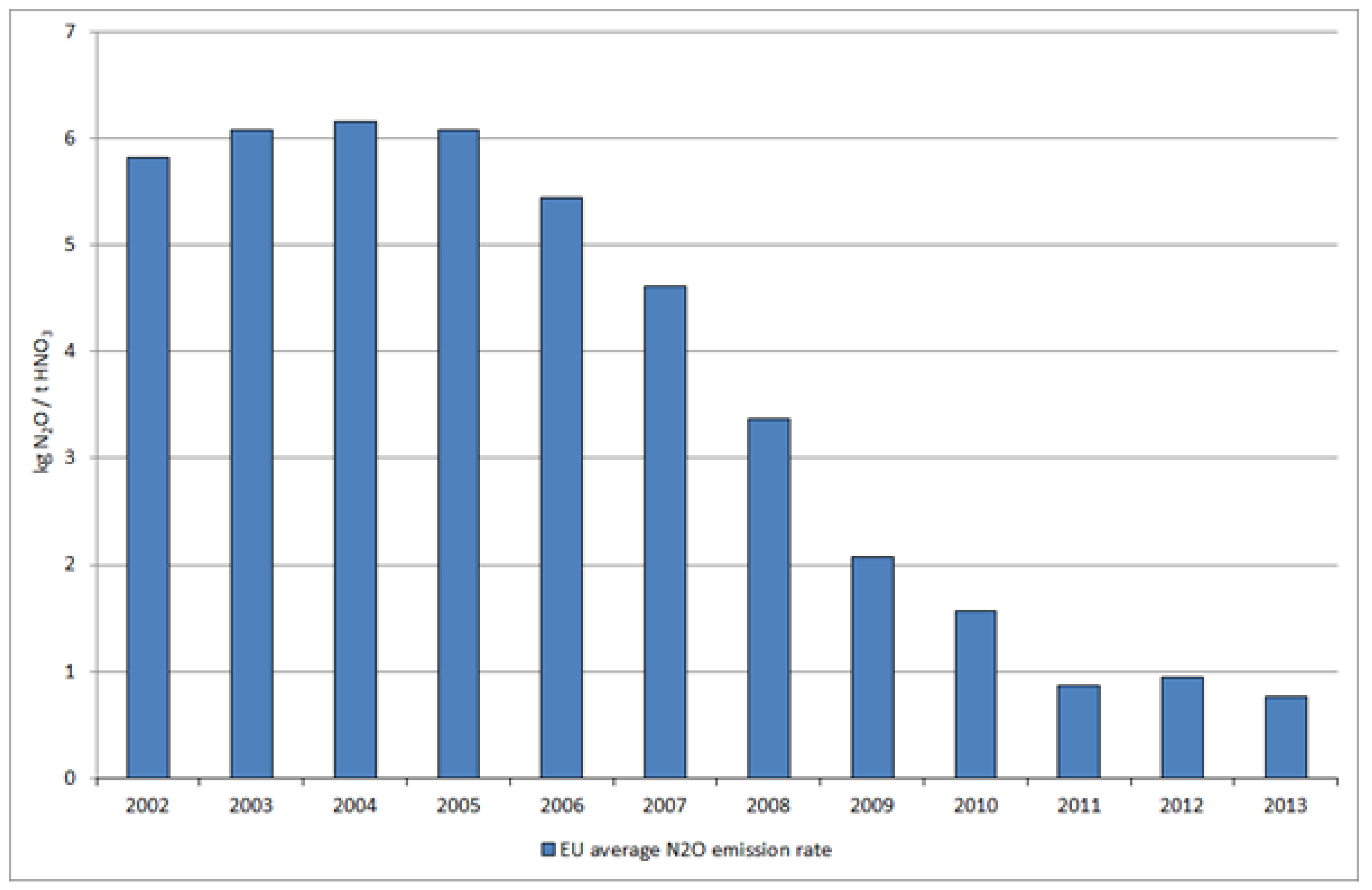
| Nitric acid | Overall emissions for nitric acid are on the rise but this is due to the fact that not all emissions were included before 2013 The specific emissions of nitric acid have been decreasing by factor of 10 since 2005, due to the availability of the catalytic reduction technology. Already in 2009, when the benchmarks were established for nitric acid, the spread across the benchmarking curve was about 300 from best to worst, indicating the availability of a reduction technology which was already in the market. The question is raised about the role of the ETS in this change as this has been triggered before nitric acid entered the ETS in 2013. However, here also the discussion on the ETS and the benchmarks before 2013 could have played an important role in the decision making processes of companies. |
© 2018 by the authors. Licensee MDPI, Basel, Switzerland. This article is an open access article distributed under the terms and conditions of the Creative Commons Attribution (CC BY) license (http://creativecommons.org/licenses/by/4.0/).
Share and Cite
Eichhammer, W.; Friedrichsen, N.; Healy, S.; Schumacher, K. Impacts of the Allocation Mechanism Under the Third Phase of the European Emission Trading Scheme. Energies 2018, 11, 1443. https://doi.org/10.3390/en11061443
Eichhammer W, Friedrichsen N, Healy S, Schumacher K. Impacts of the Allocation Mechanism Under the Third Phase of the European Emission Trading Scheme. Energies. 2018; 11(6):1443. https://doi.org/10.3390/en11061443
Chicago/Turabian StyleEichhammer, Wolfgang, Nele Friedrichsen, Sean Healy, and Katja Schumacher. 2018. "Impacts of the Allocation Mechanism Under the Third Phase of the European Emission Trading Scheme" Energies 11, no. 6: 1443. https://doi.org/10.3390/en11061443
APA StyleEichhammer, W., Friedrichsen, N., Healy, S., & Schumacher, K. (2018). Impacts of the Allocation Mechanism Under the Third Phase of the European Emission Trading Scheme. Energies, 11(6), 1443. https://doi.org/10.3390/en11061443