On the Optimal Pole Width for Direct Drive Linear Wave Power Generators Using Ferrite Magnets

Abstract

In this work, ferrite magnet linear generators for wave power applications are considered. These machines operate at unusually low speeds, around and even below 1 m/s, at which the optimal geometry differs from standard machines, since the copper loss and the force density become considerably more important. The focus is on translator design, and analytical two-dimensional (2D) expressions for the optimal 2D geometry are derived. Finite Element Analysis (FEA) is also applied to verify the analytical expressions and to determine effects from leakage fluxes and iron saturation. Demagnetization of ferrite magnets is also discussed and calculations are made to show the demagnetization situation for the magnets in different geometries. Finally, an example generator design is made to illustrate the findings. This generator is compared to three other generator concepts. It is concluded that ferrite magnet generators can have at least nearly the same shear stress as surface mounted neodymium magnet generators at low speed if the airgap is 3 mm or less, provided that a proper pole length is chosen, and that they can be economically competitive to neodymium magnet generators for wave power. It is also concluded that the demagnetization situation for the magnets can be severe, and that the choice of magnet grade and pole length is crucial in this respect.

1. Introduction

Wave power is a promising future alternative for renewable energy conversion, where the global resource has been estimated to about 2.11 TW [1] by Gunn and Stock-Williams, which corresponds to perhaps 5–15% of the world’s power demands today, depending on how large fraction of that resource that can be harvested in an economically viable way. Although the resource is large, the commercialization of wave power has this far largely been unsuccessful due to the difficulties in converting the energy at sufficiently low cost and at the same time, making the energy conversion devices durable enough so that they survive at the harsh conditions at sea. One of the key challenges is that wave energy is delivered with low speeds and large forces when compared to other renewable energy sources, such as wind power. Since the size and cost of the Power Take-Off (PTO) units, which convert mechanical power to electricity, and mechanical structures are related to force rather than power, this is unfavorable. This challenge is further complicated by the fact that maintenance is likely to be very expensive at sea, which may further increase the cost of wave power substantially.

Direct driven linear generators for wave power are PTO solutions that in principle can be made maintenance free with a proper bearing arrangement, or at least can have long service intervals. They however typically become large and expensive due to the low speeds that are involved in wave power. In principle, the size problem is two-fold and it derives from the fact mentioned above that power is speed times force, where wave power is delivered with the for power generation rather unusual combination of very large forces and very slow speeds in the order of 1 m/s. First, since the size of the generator is approximately proportional to force, not power, the power density of these machines inherently becomes low. However, any PTO system must deal with that force, and it will become rather large, although some other PTO systems, like hydraulic systems, have considerably higher force densities. Second, the slow speed makes it difficult to perform direct driven energy conversion to electricity, since the induced voltage is proportional to speed, and the resistive losses in the windings thereby become a large fraction of the total power if the current density in the windings is not reduced. By reducing the current, a higher efficiency can be achieved, but at the cost of reduced power density. Thereby, the design of a direct driven generator at these low speeds is often a trade-off between power density and efficiency.

In this work, ferrite magnet linear permanent magnet generators are considered. Ferrite magnets have poor characteristics when compared to neodymium-iron-boron magnets in almost every aspect, except cost and sensibility to heat. Rotating ferrite magnet generators have been well known for decades. Already in the 1960ies, development was made on ferrite generators [2], and Spooner was rather active in the 1990ies [3,4,5]. Even ferrite magnet transverse flux machines have been proposed [6]. Although some studies indicate that it in general does not pay off to replace neodymium magnets with ferrite magnets [7], it strongly depends on the neodymium price, and ferrites may be an alternative in situations where the larger weight of the machine is of little importance or even advantageous, provided that the actual cost of neodymium is sufficiently high so that the extra iron and winding needed is paid by the reduction in magnet cost. In recent years, the high cost, unpredictable future costs, and the scarcity of neodymium has again shed some light on the ferrite generator alternative, and linear ferrite magnet generators for wave power have been suggested, designed and built by the Uppsala group [8]. The performance of these machines is, however, strongly dependent on the pole length, and an optimization on pole length can increase the power density and/or efficiency substantially as will be evident in the remainder of this text. This is in strong contrast to the corresponding standard case where surface mounted neodymium magnets are used, where performance does not have a strong dependence on the pole length. The reason for this difference is that the flux concentrating setup of the ferrite magnets gives a different magnetic circuit compared to the surface mounted neodymium case, which introduces strong dependencies on pole length in three different aspects; the flux density in the airgap that strongly affects the power density and/or the efficiency, the demagnetization situation for the magnets, which is very important since ferrite magnets are sensitive to demagnetization, and of course the iron losses, which depend on frequency and may become substantial if the pole length is too short. All these three aspects are very important for both the initial and operational costs of the generator per kWh, the focus of this paper is to describe the first two by deriving analytical expressions that are verified by Finite Element Analysis (FEA). The iron losses are briefly addressed. Such a description has not been found for this rather special case, and although the ferrite magnet machine type itself is old the situation with extremely slow moving linear generators is in principle rather new, which motivates this article. The analytical derivation is on purpose kept simple to give clear expressions and emphasize the main point with the article, and fringing fluxes are approximated by a modification of the airgap. Further, the analysis is primarily made in two-dimensions (2D). Finally, a simple example machine is simulated and compared to other wave power generator concepts to show how important this is for ferrite generator technology and to demonstrate how much can be gained if an appropriate optimization is made.

Linear generators for wave power in general has been suggested and also built by several groups over the last two decades. Pioneers were the Archimedes Wave Swing (AWS) team who has designed and built a large generator for the AWS prototype [9]. This generator was a rather well performing Permanent Magnet Synchronous Generator (PMSG) utilizing neodymium magnets with a shear stress in the range of 40–50 kN/m². It is however designed for higher speeds, 2.2 m/s, than intended in this paper. These team members has since then explored a number of different machines, such as Transverse Flux Machines (TFM) [10], Vernier Hybrids [11], and air-cored machines [12,13]. A Vernier Hybrid has been built and tested [11], as well as an air-cored machine based on the C-gen concept [13]. The main point with the air-cored machines is that the cogging forces and the normal attraction forces between the translator and the stator are eliminated where the latter reduces the cost of the linear bearings and the structure material that would otherwise need to be dimensioned to withstand these forces. This gives a very light-weight machine. The iron losses are almost eliminated in such a machine, but a drawback is that the copper losses are instead increased since the non-magnetic gap in the magnetic circuit increases, which decreases the average magnetic flux density in the airgap. Also, considerably more magnet material is required, and the cooling capability of the copper winding is possibly lowered by the surrounding epoxy. The main point with the TFM and the Vernier Hybrids is that they have lower copper losses and higher shear stresses, which makes them very well suited for low speed applications. The drawbacks are primarily the complex and the non-standard construction (especially for the TFM) and the low power factor. The Uppsala group in Sweden has developed PMSG generators utilizing first neodymium magnets [14], and later on ferrite magnets replaced the neodymium magnets to reduce cost [8]. In the United States (US), there have also been some design and prototyping activities, where Prudell et al. have designed and built a tubular linear PMSG with the specialization that it can be run in salt water without having a seal [15]. In China, flux-switching machines have been proposed by Huang et al. to achieve some so-called magnetic gearing effect without adding the complexity of the TFM and similar machines [16]. Also, true magnetically geared machines with an integrated linear magnetic gear have been proposed by Du et al. [17] in order to reduce the low speed challenges.

2. Results

2.1. Opimalperformance for Slow Speed Wave Power Generators

For wave power generators, the involved speeds are extremely low, typically in the order of 1 m/s. Thereby, their design should be focused on reducing the copper losses and increasing the force density, which is described more in detail in Appendix A. In general, the minimization of copper losses calls for special machines, such as transverse flux machines, which implement magnetic gearing and reduces copper losses grossly [18,19]. The fraction of copper losses can be expressed as

$$p_{cu}=\frac{E_{res,RMS}}{E_{Ind,RMS}}$$

(1)

if the machine operates at unity power factor and the end windings and saturation effects are neglected. Here, $E_{Ind,RMS}$ is the average Root Mean Square (RMS) induced no-load electric field in the winding and

$$E_{res,RMS}={\rho }_{cu}J$$

(2)

represents the resistive voltage drop in the winding where ${\rho }_{cu}$ is the temperature dependent resistivity of annealed copper and $J$ is the current density. For PMSGs, the induced electric field in the winding can be expressed using the motional ElectroMotive Force (EMF), as briefly described in [20], if the end windings are neglected. With some typical geometrical assumptions, 50% iron and 50% slot in the stator, it can be shown (see Appendix A) that

$$E_{Ind,RMS}=\frac{\pi }{2\sqrt{2}}v\times {\widehat{B}}_{avg}=1.11v\times {\widehat{B}}_{avg}$$

(3)

where ${\widehat{B}}_{avg}$ is the average magnetic flux density in the airgap at direct position and a sinusoidal waveform is assumed. This expression is clearly independent on the pole length as long as ${\widehat{B}}_{avg}$ is unaffected, and it clearly shows the linear dependence between the average magnetic flux density and the induced electric field.

It is obvious from Equation (3) that the average magnetic flux density in the airgap should be maximized. However, for a neodymium magnet generator, the stator iron is typically saturated or close to saturated and it limits the flux density. For a ferrite magnet generator, the situation is quite different. Since the remanent flux density of the ferrite magnets is so low, the iron in the rotor/translator is not saturated for most geometries. In the following, a flux concentrating setup is assumed for the ferrite magnets since surface mounted configurations or similar do not give an acceptable shear stress due to the low remanent flux density of ferrite magnets. With such a configuration, the pole length has a strong impact on the magnetic flux density in the airgap, and there exists an optimum pole length for maximization. Thereby, the pole length has a profound impact on machine performance and also on the demagnetization situation for the ferrite magnets, since it affects the magnetic flux density in the magnets as well. The pole length that maximizes the flux is proportional to the square root of the airgap length as well as the square root of the width of the magnet stack, which will become evident in the analytical derivation that follows.

2.2. Optimal Pole Length for Airgap Magnetic Flux Density

To clearly illustrate the impact of the pole length on the average airgap flux density and the machine performance, the analytical approach is kept simple. The magnetic fluxes are calculated using magnetic circuit theory in 2D, where the leakage fluxes are neglected. Further, the reluctance of the iron is neglected, which is reasonable if the iron is not saturated. Saturation effects are important and limit the flux density for some geometries, but can as an approximation be taken into regard afterwards, and the flux density found with this method can be regarded as an upper limit. Thereby, a relatively simple expression of the average flux density in the airgap can be found, where the derivative with respect to pole length will yield the maximum. 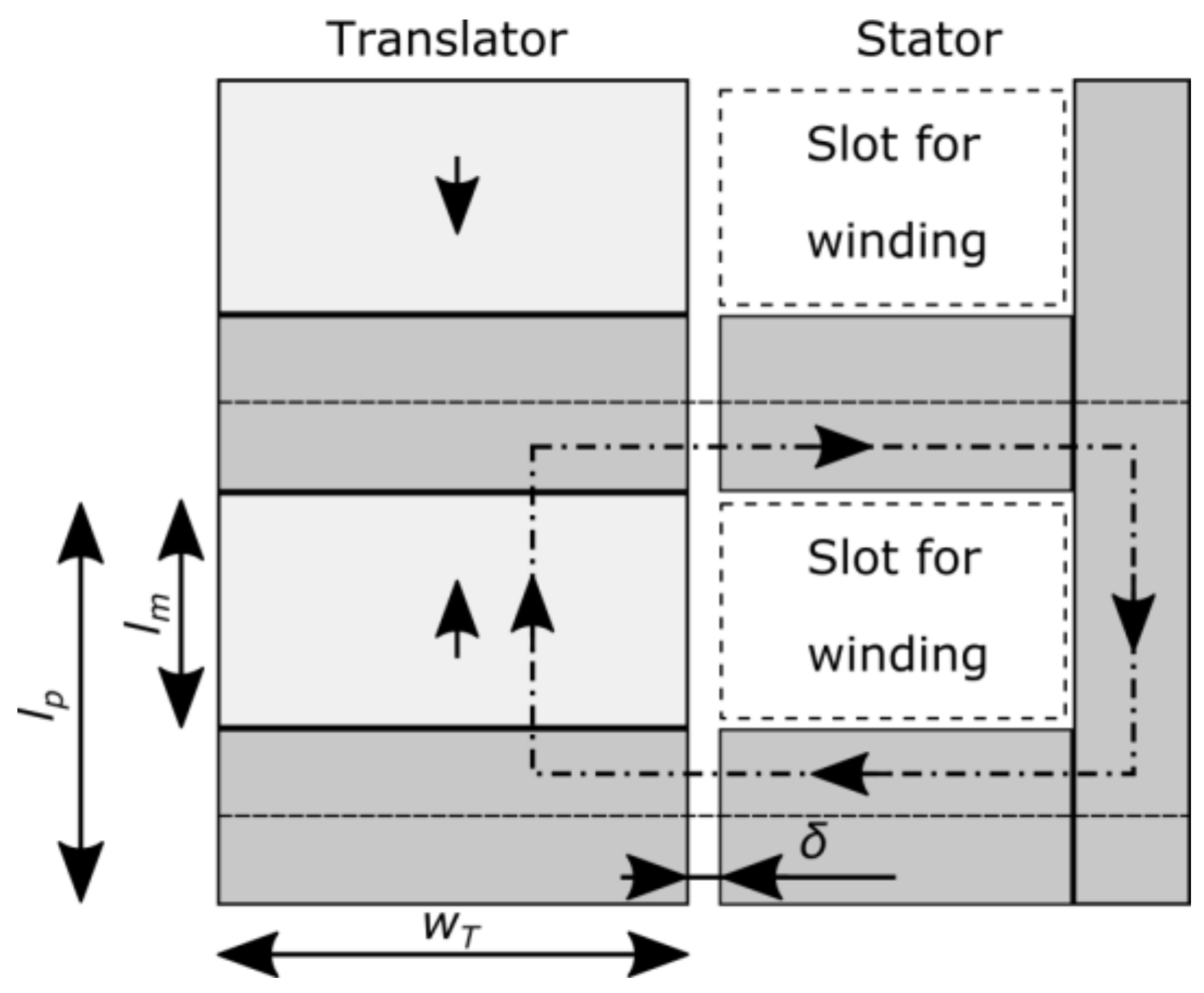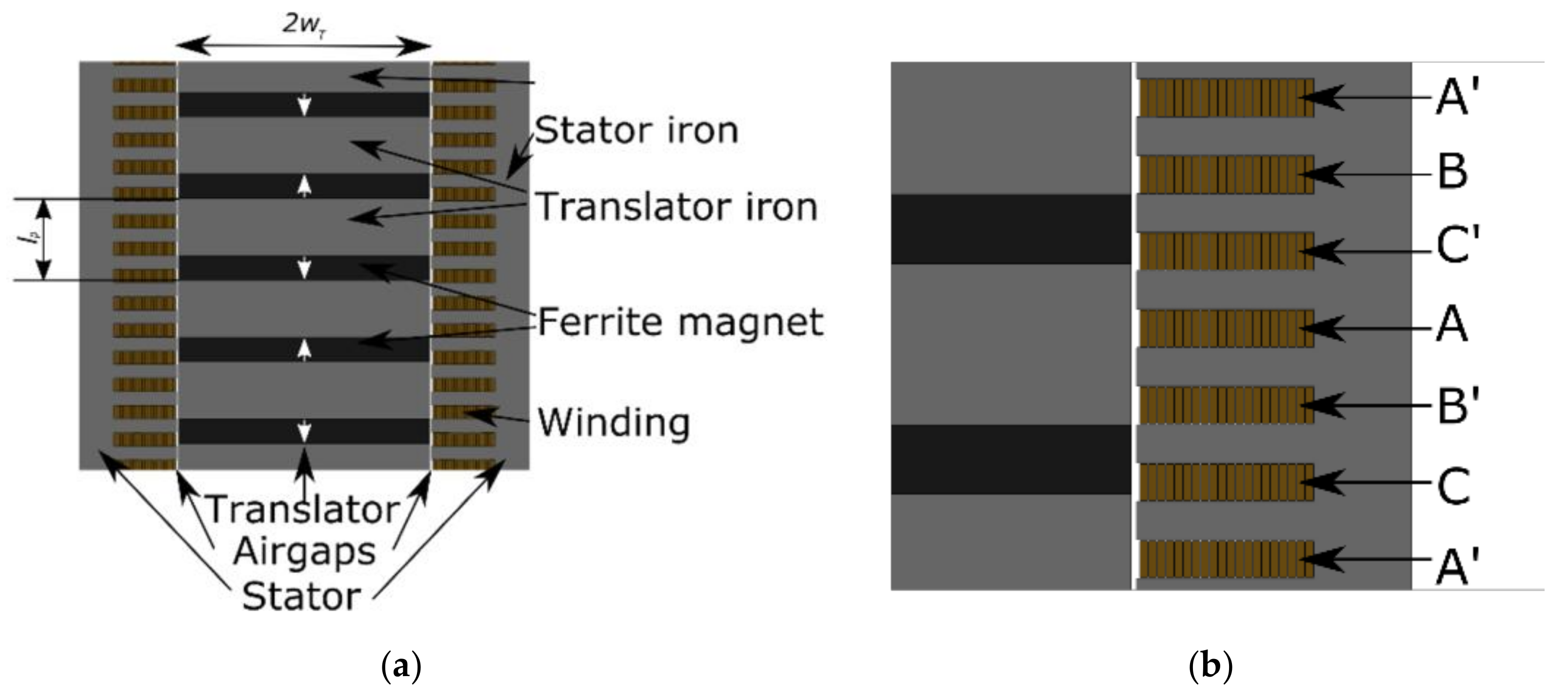In Figure 1, the cross section of a linear PMSG with ferrite magnets in a flux concentrating setup is shown, where ferrite magnets are in light grey and iron in dark grey. The stator side is simplified in the figure since its geometry anyhow will be neglected in the calculations that follow. The translator is in direct position, i.e., at d axis electrically in d-q coordinates for one phase, where the magnetic flux has its peak value at no-load. In this translator position, there is a line of symmetry between each pole where no flux passes at any position along the line, so that the boundary condition $B\cdot \widehat{n}=0$ is valid on that line. These symmetry lines are the dashed horizontal lines in Figure 1.

The magnetic circuit follows the dash-dotted line in Figure 1, where $\delta$ is the airgap, $l_p$ is the pole length, $l_m$ is the thickness of the ferrite magnets, and $w_T$ is the width of the flux concentrators in the translator. The magnetic circuit is here single-sided, and the flux leakage on the left side of the translator is ignored. If a double-sided approach is made so that a stator is placed on the left side as well, $w_T$ should be divided by 2 due to symmetry in the calculations that follow. The derivation starts from Amperes law for the free currents,

$${\displaystyle \underset{C}{\oint }H\cdot dl}=0$$

(4)

where the integral is to be taken along the dash-dotted curve in Figure 1 and the stator current is assumed to be zero. Assuming infinite permeability for the iron yields

$$H_m{l}_m+2H_a\delta =0$$

(5)

where $H_m$ and $H_a$ are the magnetic field intensity in the ferrite magnets and the airgap, respectively. Normally, the magnets operate in the second quadrant of the B-H curve. It is assumed in the derivations below that $H_m$ only assumes values on the linear part of the normal curve, and consequently that no permanent demagnetization occurs. For each particular case, it can afterwards be checked if this assumption was valid. In the linear region the magnetization can be divided into two parts, where one is the remanent magnetization $M_{m,r}$, which is independent on $H_m$ and the other part $M_{m,H}$ is proportional to $H_m$ so that $M_{m,H}={\chi }_m{H}_m$ where ${\chi }_m$ is the magnetic susceptibility of the magnet material. Then, the magnetic field intensity in the magnets becomes

$$H_m=\frac{B_m}{{\mu }_0{\mu }_{r,m}}-\frac{M_{m,r}}{{\mu }_{r,m}}$$

(6)

where $B_m$ and ${\mu }_{r,m}=1+{\chi }_m$ are the magnetic flux density and the relative permeability in the magnets, respectively. The machine is assumed to have a stacking length $l_s$ in direction into Figure 1, and combining Equations (5) and (6) yields

$$\mathsf{\Phi }=\frac{M_{m,r}{l}_m/{\mu }_{r,m}}{\frac{l_m}{l_s{w}_T{\mu }_0{\mu }_{r,m}}+\frac{2\delta }{l_s{\mu }_0(l_p-l_m)/2}}$$

(7)

where Φ = BA is the magnetic flux in the circuit, A is the cross sectional area of the block where the flux is calculated, and B is the corresponding magnetic flux density within that block, the constitutive relation $H_a=B_a/{\mu }_0$ was used and the usual reluctance terms for the ferrite magnet and the two airgaps are recognized in the denominator. Fringing fluxes are neglected in this expression, and B is assumed to be constant within any block in the magnetic circuit. Note that the height of the airgaps in the reluctance terms are only half the tooth height, since the other half of the tooth is outside the symmetry boundary and it is magnetized by another magnet. A real design is likely to have a three phase stator, which would then have several slots per pole. Thereby, the stator iron cross section at the airgap will become smaller and the airgap reluctance will increase. Also, fringing fluxes will have an impact. To approximate the effect of the tooth geometry and fringing fluxes, which are important, $\delta$ can be replaced by

$${\delta }^{\prime }=c_{s,1}\delta$$

(8)

which will be done consequently in the following, where $c_{s,1}$ is dependent on the tooth geometry and also on $\delta$ and can be expressed using the Carter coefficient [21]

$$c_s=\frac{w_{tooth}+w_{slot}}{w_{tooth}+\frac{4\delta }{\pi }\ln \left(1+\frac{\pi w_{slot}}{4\delta }\right)}$$

(9)

where $w_{tooth}$ is the tooth width and $w_{slot}$ is the slot width. The object is now to maximize the flux per unit active area with respect to the pole length, i.e., to maximize ${\left|B\right|}_{AVG}=2\mathsf{\Phi }/(l_p{l}_s)$, where it should be noted that the flux passes two airgaps. To accomplish this, the magnet length $l_m$ is set to a fraction of the pole length,

$$l_m=k{l}_p, 0<k<1$$

(10)

which yields

$$\frac{2\mathsf{\Phi }}{l_p{l}_s}=\frac{2M_{m,r}k/{\mu }_{r,m}}{\frac{k{l}_p}{w_T{\mu }_0{\mu }_{r,m}}+\frac{2{\delta }^{\prime }}{{\mu }_0{l}_p(1-k)/2}}$$

(11)

Often, the remanent flux density $B_{m,r}={\mu }_0{M}_{m,r}$ is given from the magnet manufacturer instead of the remanent magnetization, which then yields

$$\frac{2\mathsf{\Phi }}{l_p{l}_s}=\frac{2B_{m,r}k}{\frac{k{l}_p}{w_T}+\frac{2{\delta }^{\prime }{\mu }_{r,m}}{l_p(1-k)/2}}$$

(12)

The maximum of Equation (12) is found by taking the derivative with respect to pole length and setting it to zero, yielding

$$\frac{d}{d{l}_p}\left(\frac{2\mathsf{\Phi }}{l_p{l}_s}\right)=\frac{-2B_{m,r}k}{{\left[\frac{k{l}_p}{w_T}+\frac{2{\delta }^{\prime }{\mu }_{r,m}}{l_p(1-k)/2}\right]}^2}\left[\frac{k}{w_T}-\frac{2{\delta }^{\prime }{\mu }_{r,m}}{l_p^2(1-k)/2}\right]=0$$

(13)

To yield equality, the expression in the brackets to the right must be zero. This gives

$$l_p=\sqrt{\frac{4{\delta }^{\prime }{w}_T{\mu }_{r,m}}{k(1-k)}}$$

(14)

Typical values are $k=0.45$, ${\delta }^{\prime }=0.003 \mathrm{m}$, $w_T=0.2 \mathrm{m}$, and ${\mu }_{r,m}=1.1$, which yields an optimum of $l_p=10.3 \mathrm{cm}$. A half as wide stack of magnets having $w_T=0.1 \mathrm{m}$ would instead yield $l_p=7.3 \mathrm{cm}$. Note that although the flux is affected by $k$, actually mainly due to saturation effects, the optimum value of $l_p$ here is not sensitive to variations in $k$ and the variation in optimum $l_p$ is less than 9% for $0.3\le k\le 0.7$.

Having found the optimum pole length, the average magnetic flux density in the airgap can be calculated, which yields

$$B_a=\frac{{\delta }^{\prime }}{\delta }\frac{2\mathsf{\Phi }}{l_s{l}_p(1-k)}=\frac{{\delta }^{\prime }}{\delta }\frac{B_{m,r}}{\frac{l_p(1-k)}{2w_T}+\frac{2{\delta }^{\prime }{\mu }_{r,m}}{k{l}_p}}$$

(15)

where $\frac{{\delta }^{\prime }}{\delta }$ accounts for the decreased area due to the stator teeth structure. The magnetic flux density in the airgap obviously depends on the magnet grade. As an example, generic Y40 magnets are used here, which have a remanent flux density of 0.45 T and $H_c\approx -300 \mathrm{kA}/\mathrm{m}.$ There seems to be some variation in the performance of magnet grades between different manufacturers and a generic type is therefore used, which is typical, although different subcategories exist with very different $H_c.$ For $k=0.45$, $\delta =0.003 \mathrm{m}$, $w_T=0.2 \mathrm{m}$, and ${\mu }_{r,m}=1.1$, this yields $B_a=1.58 \mathrm{T},$ stating that the iron is not heavily saturated. If the model gives $B_a>1.8 \mathrm{T},$ the iron will be heavily saturated and the real value will be somewhere around 1.6–1.8 T, depending on the type of iron. A very simple model for the iron can then be employed where the maximum magnetic flux density is set to 1.8 T, giving the real value

$$B_{a,real}=\mathrm{Min} (1.8,B_a)$$

(16)

Obviously, if the saturation effects are pronounced, then $k$ can be reduced to make the iron part in the magnet stacks longer and the magnet shorter, which would reduce the saturation effects and increase the flux per unit active airgap area. In the following, the Figure 2, Figure 3, Figure 4, Figure 5 and Figure 6 assumes ${\delta }^{\prime }=\delta$ and the geometry of Figure 1 for FEA simulations for simplicity. 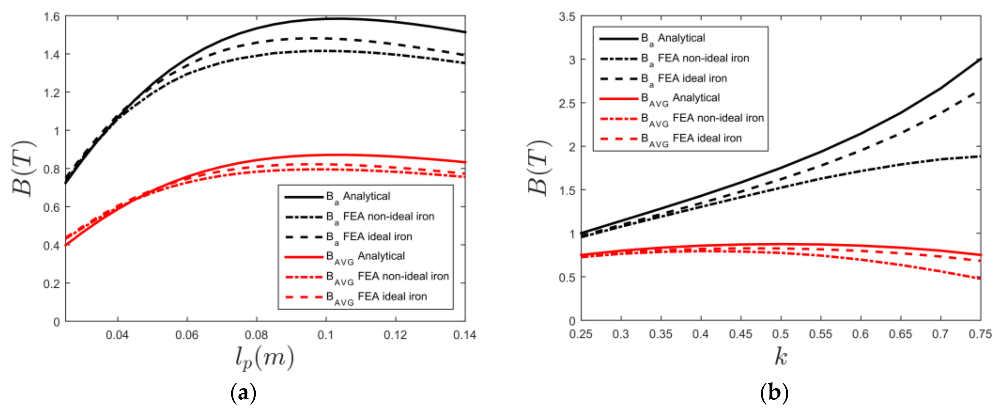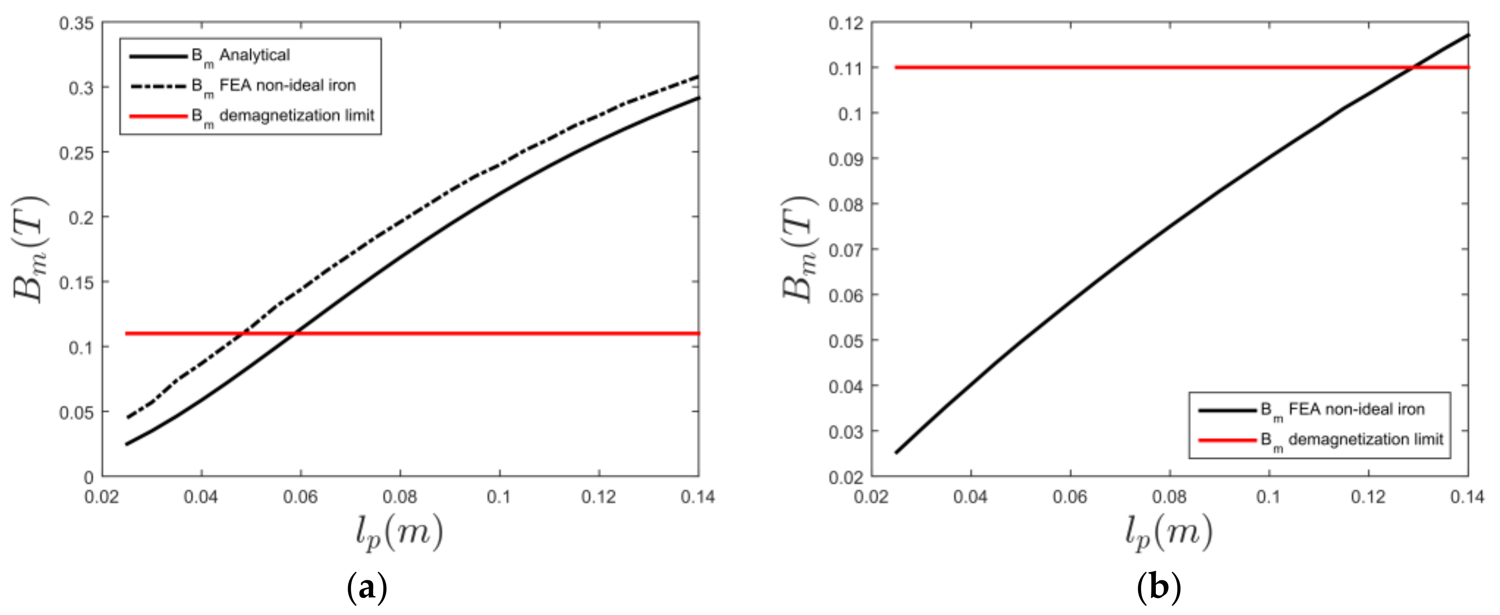Figure 2a shows how the average flux in Equation (12) and the airgap flux density $B_a$ in Equation (15) depends on $l_p$ with $k=0.45,$ and Figure 2b shows the dependence on $k$ for $l_p=0.103 \mathrm{m}.$ The parameters that are used are $\delta =0.003 \mathrm{m},$ $w_T=0.2 \mathrm{m},$ and ${\mu }_{r,m}=1.1$. 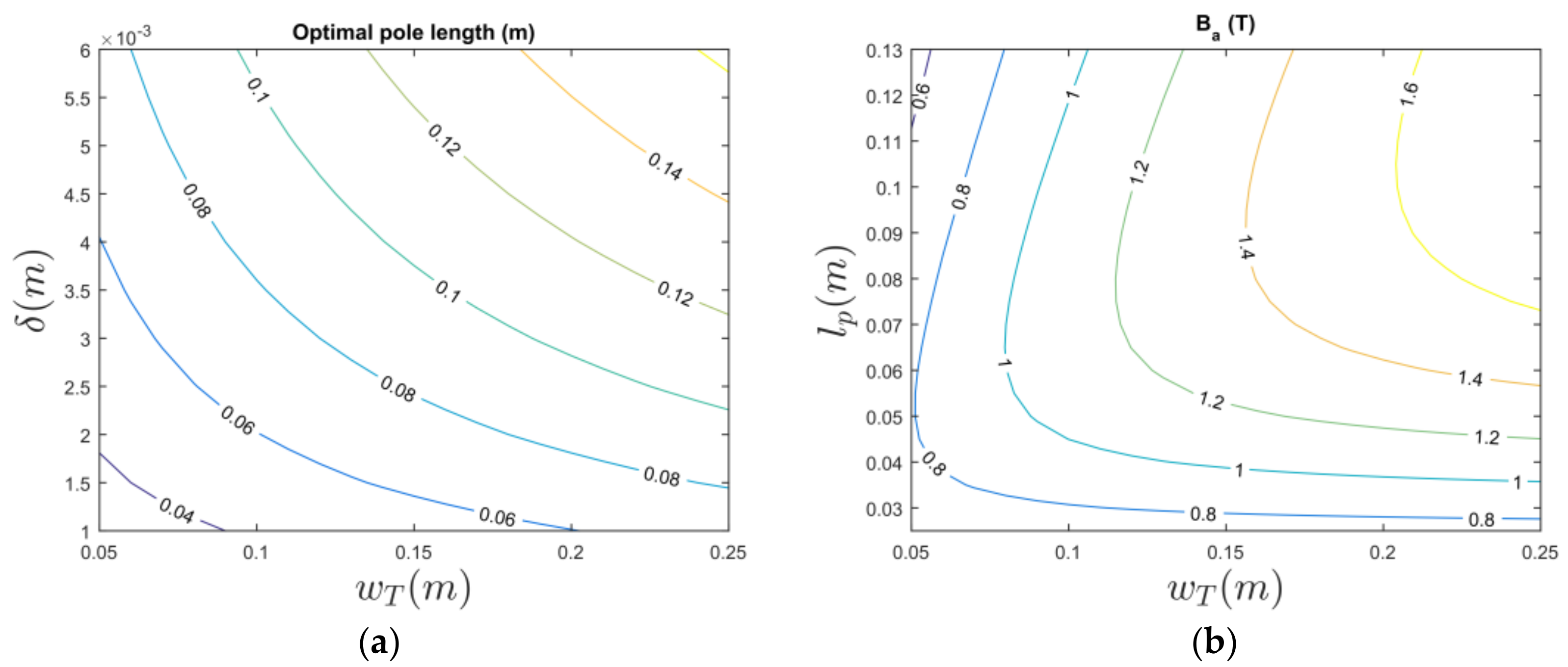Figure 3 shows contour plots of the optimal pole length from Equation (12) vs. $\delta$ and $w_T$ in Figure 3a, and contour plots of $B_a$ from Equation (13) vs. $l_p$ and $w_T$ in Figure 3b. 2D FEA simulated values has also been calculated to verify the analytical model and to illustrate the deviations that are imposed by the approximations. The FEA calculations are made both with ideal iron and iron with saturation effects to show the saturation effects clearly. The FEA calculations give higher B values than the analytical model at shorter pole lengths, since the fringing fluxes at the airgap become more important for short pole lengths. Further, the FEA calculations give lower values than the analytical model for longer pole lengths due to the increased importance of the leakage flux on the non-active side of the translator and due to the saturation effects for the non-ideal iron case. If the machine is optimized for performance, $k$ should be in the range of 0.3–0.5. Note that the cost of the ferrite magnets is in the same order as the cost for the iron, and that neither $k$ nor the pole length $l_p$ will affect the material cost significantly if the machine size is kept constant. However, shorter poles is expected be more expensive to manufacture since more parts need to be handled and manufactured, and since the cut length of the iron laminations will be longer.

The width of the magnet stack, $w_T,$ obviously has an impact on the airgap flux density $B_a$ and the performance of the machine. In Equation (7), the dependence on $w_T$ enters in the reluctance term associated with the ferrite magnet in the magnetic circuit,

$$R_m=\frac{l_m}{l_s{w}_T{\mu }_0{\mu }_{r,m}}=\frac{k{l}_p}{l_s{w}_T{\mu }_0{\mu }_{r,m}}$$

(17)

Thereby, a broader magnet stack gives a lower reluctance and a larger flux. The source expression in Equation (7), $M_{m,r}{l}_m/{\mu }_{r,m},$ is however not dependent on $w_T.$ Thereby, the magnetic flux in the magnetic circuit can be increased by increasing $w_T$, as long as the reluctance of the magnet $R_m$ is of significant magnitude when compared to the total reluctance in the magnetic circuit. If the airgap reluctance is considerably larger than $R_m$ or if the iron is saturated, then the flux cannot be significantly increased by increasing $w_T.$ There is also a limit on how low the magnetic field intensity in the magnet $H_m$ can become due to demagnetization, which limits the geometry for many of the ferrite magnet grades. As an example, the generic Y40 grade with $H_c=-300 \mathrm{kA}/\mathrm{m}$ is used, which corresponds to a magnetic flux density in the magnets $B_{Demag}\approx 0.11 \mathrm{T}.$ Since

$$B_m=\frac{R_m}{R_m+R_a}{B}_{m,r}$$

(18)

where

$$R_a=\frac{2{\delta }^{\prime }}{l_s{\mu }_0{l}_p(1-k)/2}$$

(19)

is the reluctance of the two airgaps in the magnetic circuit, the lower bound on $R_m$ becomes with $B_m=B_{Demag}$.

$$R_m=\frac{B_{Demag}}{B_{m,r}-B_{Demag}}{R}_a$$

(20)

Inserting $B_{m,r}=0.45 \mathrm{T}$ and $B_{Demag}\approx 0.11 \mathrm{T}$ yields

$$R_m=0.32R_a$$

(21)

The airgap length ${\delta }^{\prime }$ is obviously an important parameter, and the average airgap flux density and the power density of the machine is strongly dependent on the airgap. In fact, ferrite magnet generators are considerably more sensitive to variations in the airgap when compared to neodymium magnet generators in the sense that the average flux density in the airgap will drop considerably faster for the ferrite magnet generator when the airgap is increased. This can directly be seen from the magnetic circuit or from Equation (12). In a typical surface mounted neodymium magnet generator, the magnet is several times thicker than the airgap. Thereby, the main reluctance in the magnetic circuit is associated with the magnet itself, and the airgap reluctance is only a smaller fraction of the total reluctance. A small increase in the airgap would, in this case, only modify the reluctance and the flux slightly. For the ferrite case, the airgap constitutes a major part of the total reluctance in the magnetic circuit, especially if the pole length is short. A small increase in the airgap will therefore increase the reluctance and decrease the airgap flux at a possibly several times higher rate for a ferrite generator than for a surface mounted neodymium magnet generator. For really short pole lengths, where

$$\frac{R_a}{R_m}=\frac{4{\delta }^{\prime }{w}_T{\mu }_{r,m}}{l_p^{2}k(1-k)}>4$$

(22)

the magnet reluctance can almost be neglected in the magnetic circuit and the average flux density in the airgap then becomes inversely proportional to the airgap. Thereby, the power density of the machine becomes proportional to $1/{{\delta }^{\prime }}^2$ if the fraction of copper losses is kept constant. This is an important observation, since the long translators and the stators in linear machines are difficult to manufacture with precise accuracy. For typical values $k=0.45$, ${\delta }^{\prime }=0.003 \mathrm{m}$, $w_T=0.2 \mathrm{m}$, and ${\mu }_{r,m}=1.1$, Equation (22) holds for $l_p<52 \mathrm{mm}$. The normal negative magnetic stiffness of the translator is also affected by this, which is a drawback for the ferrite generators when compared to the neodymium case. The normal forces on a symmetric translator will simply not cancel as efficiently if the translator is displaced as compared to the neodymium case, since the flux density on the opposing sides will differ more. Thereby, the net normal force will become considerably larger for ferrite generators when compared to the neodymium case if the machines have the same power rating, which increases the bearing cost.

2.3. Demagnetization of Ferrite Magnets

Ferrite magnets are not only several times weaker than neodymium iron boron magnets in terms of remanent flux densities. Most ferrite magnet grades are also considerably more sensitive to demagnetizing magnetic fields, and if the internal magnetic flux density is lowered below a certain level permanent demagnetization will occur. Nowadays, however, there exist ferrite magnet grades with decent remanent magnetization that can withstand zero flux densities or even reversed fields without experiencing permanent demagnetization. As will become evident below, the choice of magnet grade is very important for ferrite magnet generators. Note here that for rather substantial permanent demagnetization to occur in many grades of ferrite magnets, the magnetic flux density field does not need to be in the opposite direction of the remanent magnetization. It is sufficient that the magnetic flux density in the magnet $B_m$ falls below the original threshold value for demagnetization $B_{Demag}$, and the remanent flux density would then approximately be lowered by $B_{Demag}-B_m$, as well as the threshold value $B_{Demag}$. 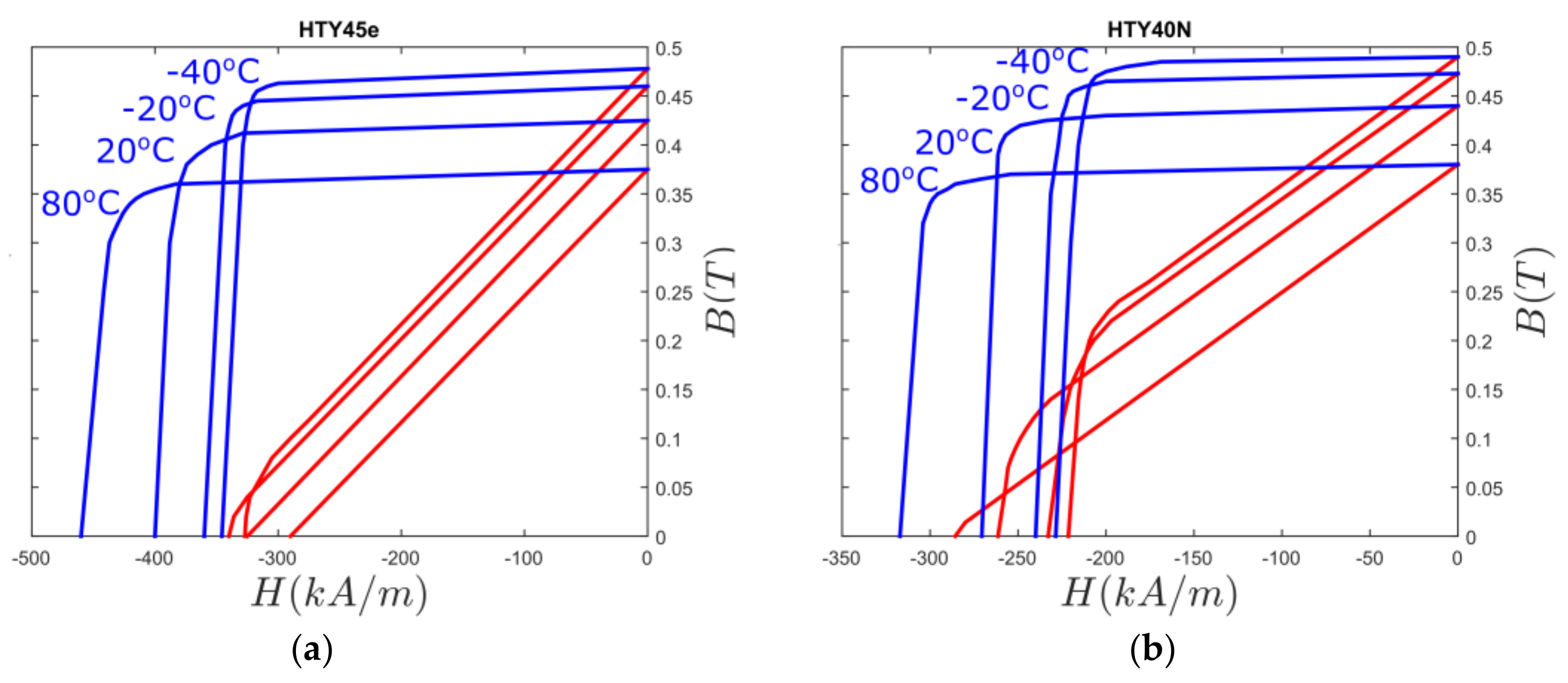Thereby, not only the current loading may cause demagnetization, but also the shape of the magnets and the geometrical layout. The magnet can simply be demagnetized by other parts of the magnet or by other magnets. The demagnetization is permanent, and it is sufficient that the demagnetizing flux density is reached on one single occasion for demagnetization to occur. A very sensitive such case is the mounting process, which actually may produce the lowest magnetic flux densities inside the magnet that the magnets will experience during their lifetime if the magnets are short and broad. To illustrate this, the B-H curves in the second quadrant for two different ferrite magnet grades, HTY45E and HTY40N, are shown in Figure 4, where HTY40N is sensitive to demagnetizing fields at room temperature, but HTY45E is not.

In the simplified analytical approach, the magnetic flux density in the magnet can be calculated by distributing the flux evenly in the magnet. This yields

$$B_m=B_a\frac{l_p(1-k)/2}{w_T}=\frac{B_{m,r}}{1+\frac{4w_T{\delta }^{\prime }{\mu }_{r,m}}{(1-k)k{l}_p^2}}$$

(23)

The dependence on pole length for $B_m$ for values $k=0.45,$ ${\delta }^{\prime }=0.003 \mathrm{m},$ $w_T=0.2 \mathrm{m},$ and ${\mu }_{r,m}=1.1$ is given in Figure 5a, where also the demagnetization limit for the generic Y40 magnets $B_{Demag}=0.11 \mathrm{T}$ is plotted. As can be seen, at normal operation the magnets get demagnetized even at no-load if the pole length is shorter than 5 cm, but is safe with a margin at the optimal pole length 10.3 cm. For example, for a pole length of 3.5 cm, it seems that the remanent flux density of the magnets would be reduced by about 0.04 T from 0.45 T to 0.41 T for the FEA calculation, which is 8.9%, just by being in the stator. However, considerably more severe demagnetization situations will be experienced by the magnets. For a linear machine, most of the translator normally leaves the stator at some position during a full stroke since the translator is normally longer than the stator. This lowers $B_m$ significantly since the iron path in the stator no longer conducts the flux, especially for the longer pole lengths, and it should be taken into regard. The simple analytical model cannot however be used to analyze this case, and FEA analysis is required. In Figure 5b, $B_m$ is shown for the same translator when the stator is not present. As can be seen, permanent demagnetization will happen even at the optimal pole length 0.103 m, but it is considerably less severe than for the shorter pole lengths. Note, however, that 3D effects will lower the strain on the magnets and will increase $B_m,$ depending on how large $l_s$ is. Also, the demagnetization effect is rather insignificant for pole lengths that are longer than 0.1 m.

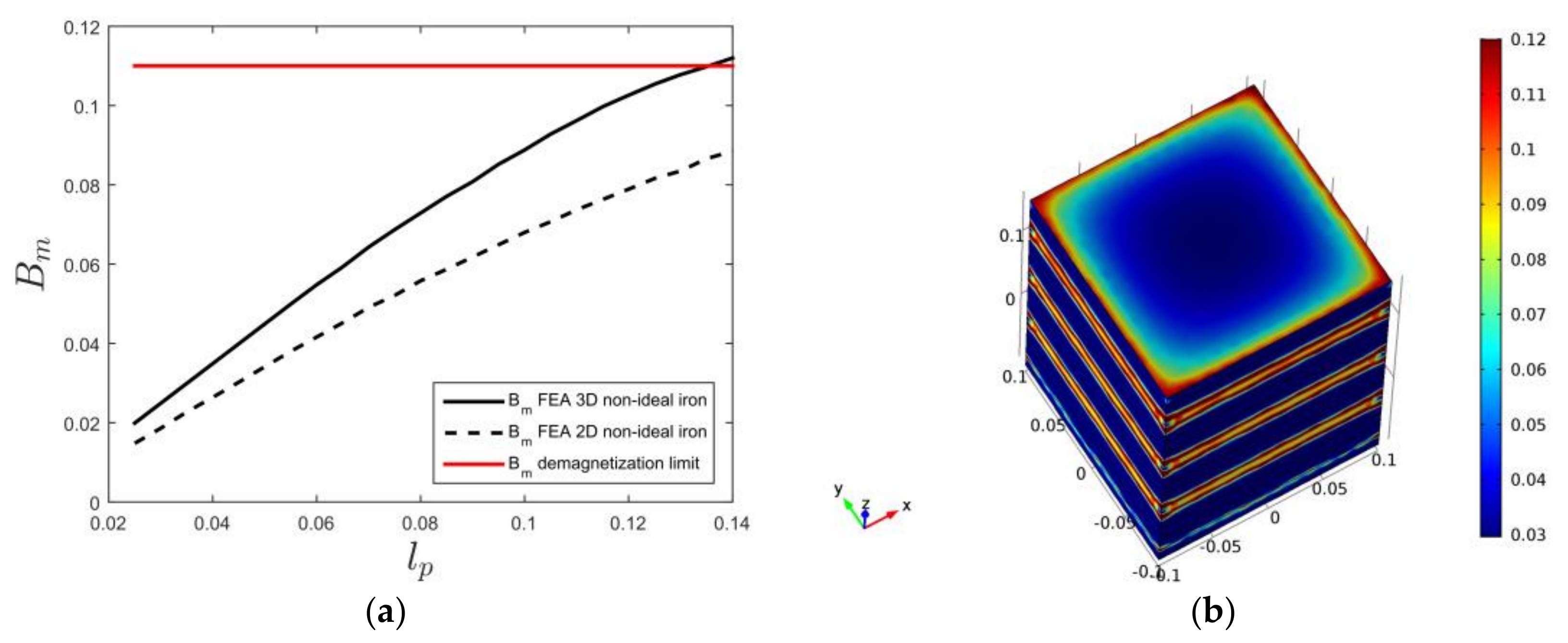
Finally, the demagnetization effects during manufacturing and mounting are considered. As is well known, the individual magnets must not be too wide when compared to how long they are in the direction of magnetization. If they are, they will suffer from demagnetization already when they are magnetized during the manufacturing process. This can easily be checked in a FEA program, such as Comsol Multiphysics, or by examining the load line in the magnetic circuit. However, the mounting process is also a hazardous step that may cause demagnetization. This can be illustrated by just adding a number of poles on the translator and leaving the top iron layer unmounted. Then, the magnetic field in the top magnet layer will become lower in the center of the magnet when compared to the fully mounted case since no iron will help to conduct the flux from the center of the top to the translator edge. A simulation is shown in Figure 6a, where both 2D data and 3D data with $l_s=w_T$ are shown to show the 3D effects. Note that the demagnetization situation is significantly improved with the quadratic translator in 3D, but that also the shear stress is decreased when compared to the 2D case. In Figure 6b, the z component of the magnetic flux density in the magnets is shown in 3D for a short pole length of 35 mm. As can be seen, demagnetization can be severe for sensitive magnet grades everywhere in the magnets except at the outermost cm or so, if not, special measures are taken to avoid this during mounting. One such measure would actually be to heat the magnets before mounting (see Figure 4).

2.4. Suggested Machine Design

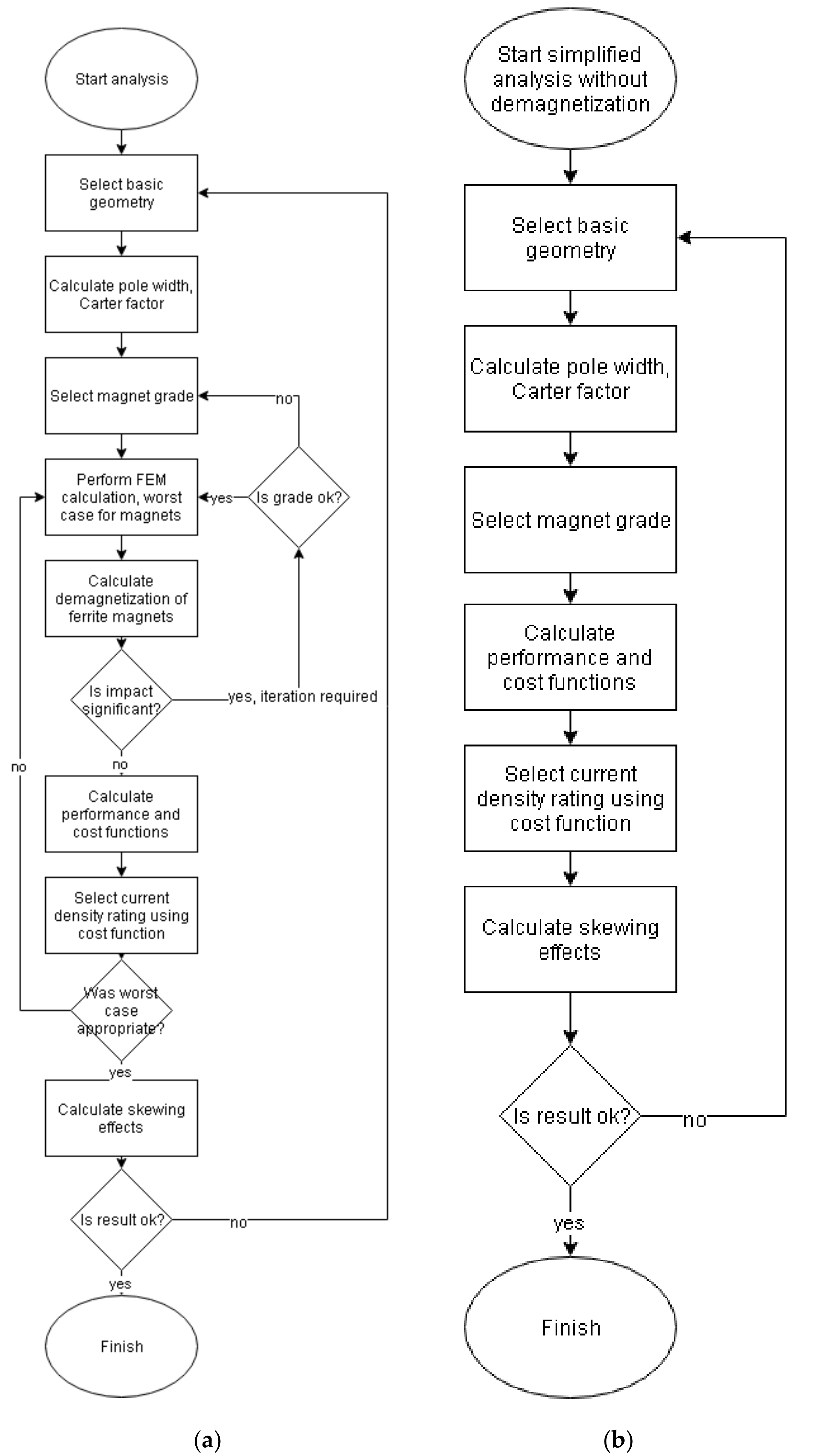
To illustrate the results in the previous sections, a simplified 2D electromagnetic design of a three-phase machine with 3 mm airgap is made, using the generic Y40 ferrite magnet type. The design procedure can be done in many different ways. In Figure 7, the flow chart for the design process that was used in this work is given. There are two flow charts, one that regards demagnetization effects in Figure 7a and one simplified that does not in Figure 7b. In this work, the simplified flow chart is followed, since we do not currently have a demagnetization code available. A detailed demagnetization analysis is complex, since the skewing should preferably be taken into regard. In the last step, the design can be iterated numerous times to increase properties, such as the no-load voltage total harmonic distortion (THD), typically by changing k, and to optimize total cost per kW. In a full final design, the full analysis is preferable to follow before a machine is built where the demagnetization effects on the magnets are analyzed in detail for different magnet grades, and a cost analysis is made to choose grade. Also, iterations in the last step should be done to fine tune optimization in combination with the demagnetization analysis.

An illustration of the design is shown in Figure 8. The width of the translator is selected to 400 mm with a double-sided flat approach so that a symmetry line is found at the center of the translator, giving $w_T=0.2$ m. The stator design is more or less copied from the work of Polinder et al. [9,10], which is well optimized for a neodymium magnet translator. This design has three teeth per pole, and to allow for flux to pass through all three teeth simultaneously a low value of k = 0.3 is selected for the machine, which gives a long iron part and a short magnet. Further, we select the height of the slots to be the same as the height of the teeth, $l_p/6$, and we assume a slot fill factor of 65%, assuming that rectangular copper bars are used. The slot depth is set to 100 mm. To find the optimal pole length in Equation (13), the Carter factor in Equation (9) is required, which in turn depend on the pole length. A few iterations (4 is sufficient) solve this to sufficient accuracy, which yields $\delta \prime =4.53 \mathrm{mm}$ and $l_p=138 \mathrm{mm}$. At direct position more teeth than slots are occupying the airgap, and the Carter coefficient then slightly overestimates the optimal pole length. We therefore round down to $l_p=130 \mathrm{mm}$ for the suggested machine. The mechanical design is assumed to be similar to the one in [9,10], which has been built.

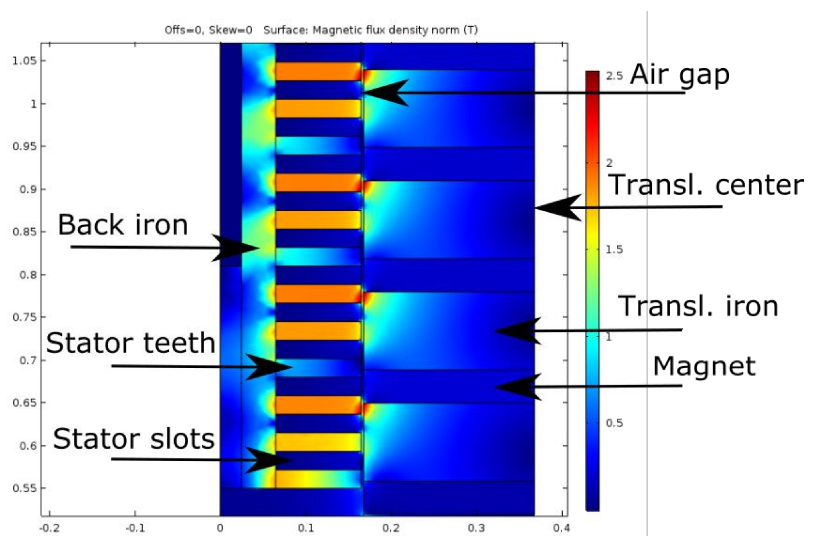
A FEA 2D simulation of the machine in direct position for phase A is shown in Figure 9, where the RMS current density is 2.5 A/mm². Skewing is employed to reduce the cogging and force ripple, which would otherwise have an unacceptable amplitude in the order of 25–50% of the maximum force. Figure 9 shows the non-skewed case. The skewing is performed linearly over a third of a pole, i.e., over one whole tooth and slot. Then, only the end effects of the cogging force remain. The skewing reduces the power with about 3%, but reduces the cogging/force ripple amplitude to about 3–4% of the maximum force that is acceptable.

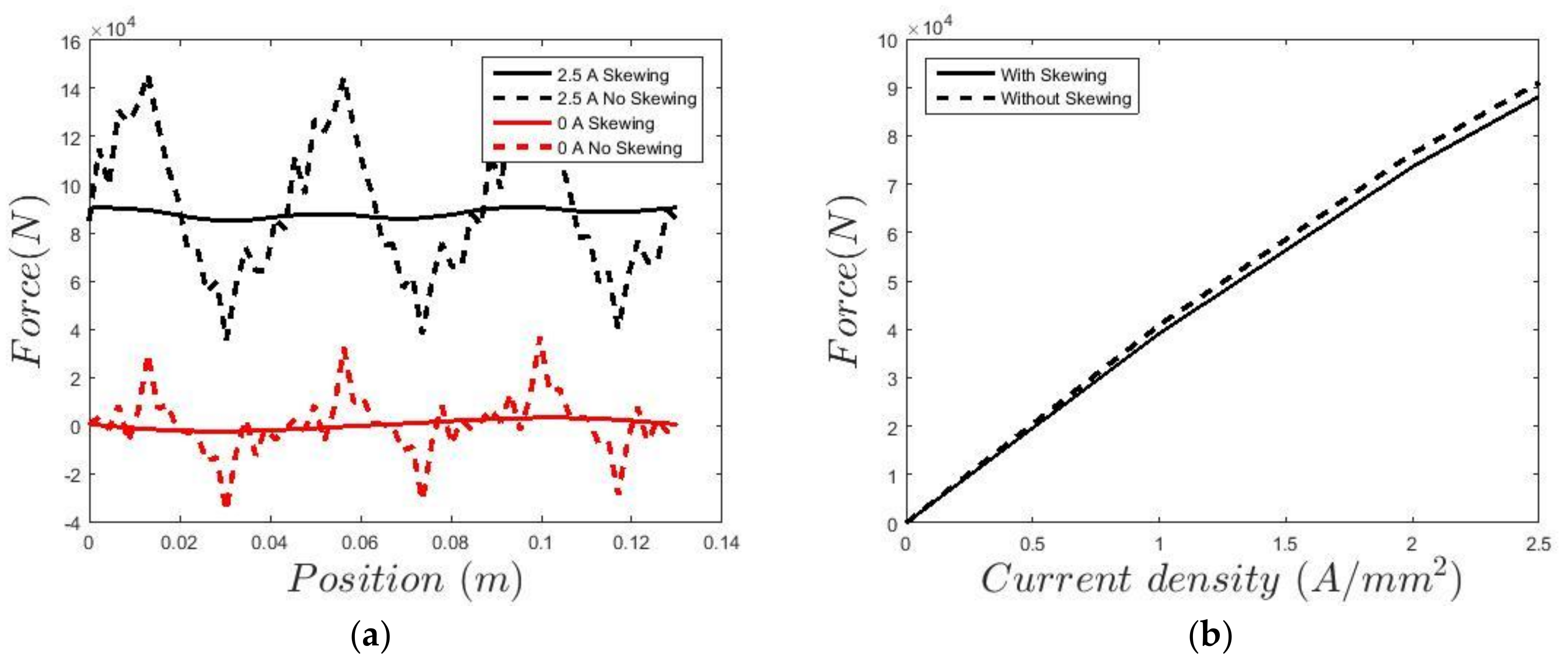
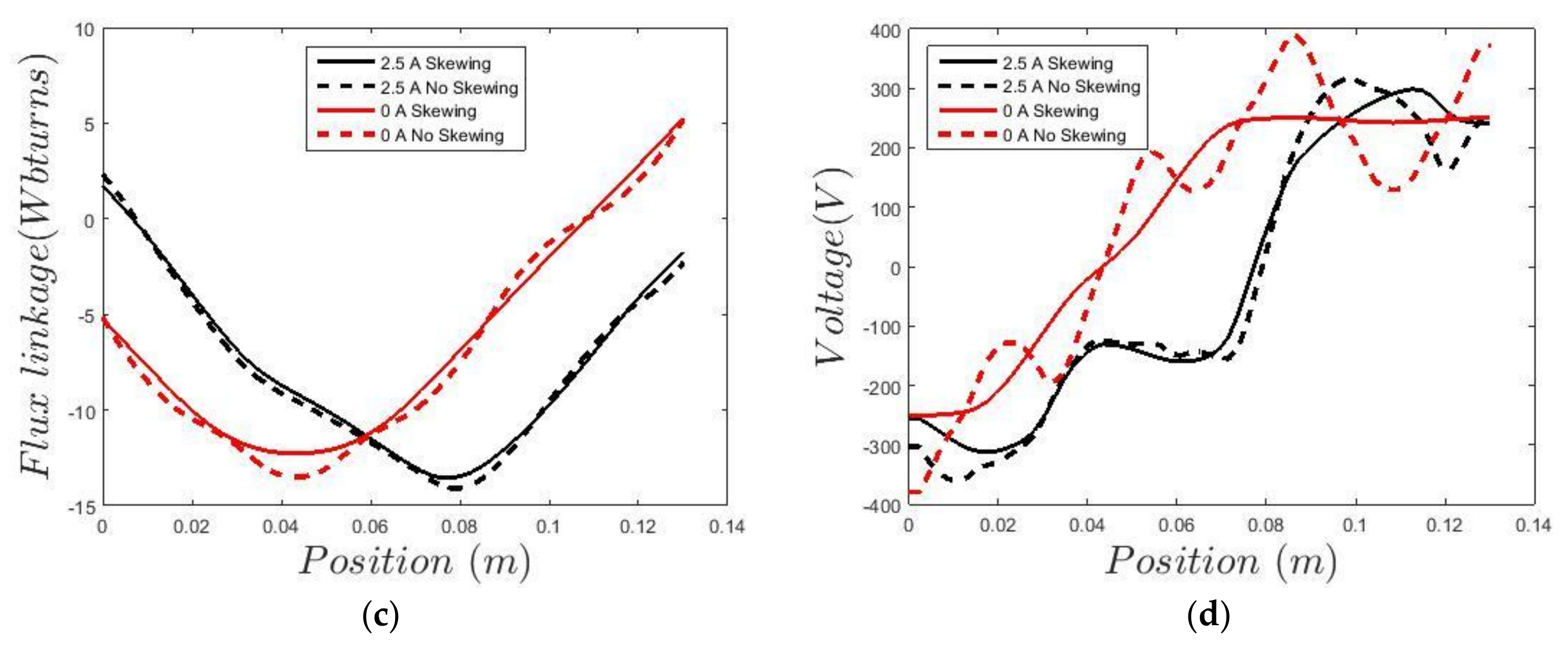
The force, voltage and flux linkage characteristics of the ferrite generator are shown in Figure 10, where the current is sinusoidal having only a q component.

The stator is made 2.08 m high, i.e., with 16 poles. The machine is designed for 1 m/s, and a current density of only 2.5 A/mm² is used to retain copper losses at a reasonable level. Note that if the slot fill factor of 0.65 cannot be reached, then the current density should instead be increased resulting in larger copper losses. Already at 2 A/mm² saturation effects start to show, and increasing the current density from 2 to 4 A/mm² only increases the damping force with 62%. For the winding, 20 turns and a slot depth of 100 mm is assumed. This gives a current rating of 114 A. Further, a stacking width of 0.5 m is assumed, which gives an active airgap area of 2.1 m² in total for both sides. The simulated performance of this machine is given in

Table 1. Properties of the designed generator.

Parameter	Value	%
Rated speed	1 m/s	-
Pole width	130 mm	-
Frequency	3.85 Hz	-
Rated EM force	88 kN	-
Shear stress	42 kN/m2	-
Stator iron mass	1540 kg	19.4%
Stator Cu mass	812 kg	10.1%
Translator iron mass	4420 kg	55.2%
Magnet mass	1230 kg	15.3%
Total active mass	8002 kg	-
Rated power	76 kW	-
Copper loss	12.1 kW	13.8%
Iron loss	630 W	0.7%
Friction loss	1 kW	1.1%
Efficiency at 1 m/s	-	84.7%
Efficiency at 0.7 m/s	-	78.9%
No-load voltage 1	208 V	-
Phase current	176 A	-
Phase resistance	0.12 Ω	-

¹ Voltage is non-sinusoidal.

, where 3D effects are not included. Since the iron losses are small when compared to the copper losses, a very simple model for the iron losses is assumed. The losses per kg are separated into hysteresis losses and eddy current losses, where the hysteresis losses are assumed to be proportional to frequency, 2.5 W/kg at 50 Hz, 1.5 T, and the eddy current losses is assumed to be proportional to frequency squared, 2 W/kg at 50 Hz, 1.5 T. After applying the frequency, this value is multiplied with a build factor of 2 to take manufacturing effects and non-sinusoidal fields into account, and then just multiplied with the stator iron mass. The resistivity is assumed to be $2.13\times {10}^{-8} \mathsf{\Omega }\cdot \mathrm{m}$, corresponding to annealed copper at 80 °C. To account for end windings, the winding resistance, copper losses and copper mass are multiplied with a factor 1.35. The bearing system is very roughly assumed to add 1 kW friction losses, corresponding to rather well balanced steel rollers. The iron losses in the translator are not included. The stroke length is considered to be 2 m, which gives a translator that is 4.1 m.

To get an idea of how serious the demagnetization problem is, a simplified approach has been made. A manual investigation on the internal fields in the magnets at full load shows that the bulk of the magnets are safe with a margin at normal operating conditions when the translator is inside the stator, as consistent with results in Figure 5a. When the translator is outside the stator, the bulk of the magnets have a magnetic flux density of 0.05 T, indicating that some permanent demagnetization would take place if the generic Y40 magnet type is used. Thereby, up to 10% of the magnetization could be lost. This can be avoided by using the magnet type HTY45E, see Figure 4a, although they are a more expensive ferrite grade. It is also worth noting that the translator should not be stored outdoors during cold winters. The demagnetization effects would then become larger due to the temperature dependence on the coercivity, see Figure 4. Further, the corners of the magnets become demagnetized to various extent in an area approximately formed like a triangle with 10 × 10 mm sides due to the current loading. This would also affect HTY45E magnets, but to a lesser extent. By assuming that the remanent magnetization completely disappears in these triangles, a pragmatic (although not strict) worst case scenario for this demagnetization can be simulated. The results show that the shear stress is then reduced to 35 kN/m² at full load, corresponding to a reduction of 16.7%. This is rather severe, but the real case should most likely be less severe, probably considerably less.

2.5. Comparison to Other Generators

To put the ferrite generator design into perspective, it is compared to three other wave power generators, where two have already been designed and built and one is under construction. The machine in this paper is called machine A. The other machines are:

• Machine B. The neodymium magnet generator designed and built by Polinder et al. for the Achimedes Wave Swing, from [9,10].
• Machine C. The ferrite magnet generator L12 designed and built by the Uppsala group [8].
• Machine D. The generator of transverse flux type given in [18,19] which is currently being built by the author.

To compare the generators, they are all simulated in FEA at unity power factor with a sinusoidal current that is in phase with the no-load voltage. This, in general, gives higher shear stresses than presented/indicated in [8,9,10] for a certain current density, and assumes that an active rectifier is present. The speed is set to 1 m/s for all of the machines. To compare the cost of the generators, active material costs, and costs for losses are approximated. Note that these costs may differ significantly from the real costs of the machines, and mainly should be regarded as a tool for comparison. Optimization of the structure by selecting geometry is, for example, important to push down costs, but is not regarded. This has most likely been done for machine C. It can, however, be done in the same way for all the machines A, B, and C, and will not affect the comparison of these. Machine D look very different [19]. Maintenance costs, installation costs, etc. is considered to be the same for all machines, although the ferrite machines are heavier, and are not included in the comparison. The assembly costs are not regarded. The cost is expressed in costs per kN shear force, where the translator for simplicity is assumed to be twice as long as the stator for machines A–C. Note that the simulated size for machines A–C is not important as long as the end effects are negligible, since the cost of the active materials per kN is largely unaffected by size. For machine D, costs are more dependent on size. In this comparison, 2.1 m stroke is assumed for machine D, as consistent with machine A, and 200 kN damping force as given in [18,19] is used for material and efficiency calculations. The active material costs are estimated from the mass of each material per kN shear force multiplied with the approximated costs/kg given in

Table 2. Material costs in €/kg and densities.

Material	€/kg	Density (kg/dm³)
Translator iron	1.5, 3 for machine D	7.7
Stator iron	3	7.7
Ferrite magnet	3	5
N42 magnet	50	7
Copper	9	8.9
Aluminium winding	4.5	2.7

. Also, the densities that were used for the materials are given in Table 2. The structural design is not addressed in the design of machine A, and not published in detail for machines B, C, or D. To give some crude indication of the difference in structure cost between the different machines, it is observed that the weight and cost of the structure is to a large extent dependent on the clamping magnetic normal forces between the two stator sides per kN shear force, which differ between the machines that are compared here. The normal force per kN shear force is

$$F_{N,norm}=\frac{{\sigma }_N}{{\sigma }_s}$$

(24)

where ${\sigma }_N$ is the normal stress and ${\sigma }_s$ is the shear stress at the airgap. For machine D, the average normal stress is used since it has several airgaps of different type. The structure cost is also dependent on machine size per kN shear force, i.e., the structure will become larger for machines with low shear stresses, since the beams then will become longer and thicker.

The linear bearings are also costly components. Plain bearings are robust and low cost, but they have typically 20 times larger friction losses than roller bearings. Thereby, roller bearings will be considered here. Since the normal forces on the translator ideally cancel with a symmetric construction, the bearings are dimensioned by the change in magnetic normal force on the opposing sides due to a small translator displacement, i.e., the negative magnetic stiffness (or spring constant) of the translator. Since this parameter differs grossly for the machines that are investigated, the bearing costs will be different. The translator weight also affects bearing costs, since the lowest mechanical resonance frequency should preferably be avoided. The bearing cost is of course complex and depends a lot on design. Especially, the racetracks need to have fine tolerances since the stiffness of the roller bearing mountings need to be high to counteract the negative magnetic stiffness with a margin. If the race tracks are not precise, then the fatigue load limit of the bearings will be violated due to the stiffness of the mountings and the bearings will eventually break. The tolerance requirements on the racetracks are considerably stricter than those on the airgap in the magnetic circuit. The bearing cost is not modelled here, since it is regarded to be too complex and a simple model will be misleading to readers. However, the cost is indicated by calculating the negative magnetic stiffness per kN shear force,

$$c_{bearing}=\frac{k_{mag}}{{\sigma }_s}$$

(25)

where $k_{mag}$ is the negative magnetic stiffness per m² active airgap area on each side of the machine, so that the net force on the translator per m² active airgap area for a displacement $\Delta l$ becomes

$$F_{tr}=\frac{1}{2}{k}_{mag}\Delta l$$

(26)

where the factor ½ takes into account that there are two sides.

The negative magnetic stiffness of the translator is best calculated using FEA analysis by simply displacing the translator 0.5 mm sideways and calculating the change in normal force. Except for machine D, tests were also made with 1 mm displacements in order to verify the approximate linearity of $k_{mag}$. The negative magnetic stiffness of the translator also set stiffness and strength requirements on the translator structural design, especially for machine D. This is not further pursued here, but is discussed in [18,19].

The frictional losses generally depend on bearing type and the required pretension of the bearings. They are generally hard to determine, and they are modelled by setting the friction losses of machine A to 1.1% from Table 1, which is a reasonable level. The friction losses for machines B and C are modelled by scaling them linearly with $c_{bearing}$, so that the fraction becomes $0.055+0.055\hspace{0.17em}{c}_{bearing}/c_{bearing,A}$ where $c_{bearing,A}$ is the negative magnetic stiffness per kN shear force for machine A. Machine C does not have steel rollers, but rubber wheels [22]. This will increase friction grossly, which is indicated in [23], but steel wheels will be assumed for all of the machines in this comparison. For machine D, friction loss is set to 0.5% from [19], which is possible for this machine despite the high $c_{bearing}$ due to some mechanical tricks that has been implemented, which are not straight forward to implement on the other machines.

The iron losses and copper losses for machines B–D are calculated in the same way as for machine A. The losses per kN are valued assuming a rated speed of 1 m/s, giving 1 kW/kN. The machine is assumed to operate with linear damping, so that the damping force of the generator is proportional to speed. This is a typical operation scheme for point absorbers, where the damping force then is typically matched to the hydrodynamic radiation force. An additional control force can increase the power output significantly, but is here assumed to be provided by another system. With linear damping, the fraction of copper losses, iron losses, and friction losses, i.e., in % of the power, remains approximately independent on speed if the shear stress can be assumed to be proportional to the current. Thereby, the losses can be calculated with an assumed utilization factor for the power rating. Here, 15% is selected for comparison purposes for the rating at 1 m/s, and 20 years of operation. The electricity cost is assumed to be €0.1/kWh, and the price of electricity is, for simplicity, assumed to increase as much as the interest rate. Thereby, 1% of losses cost 26.3 €/kN. Performance and costs per kN shear force for machines A–D is summarized in

Table 3. Cost and performance comparison of the four machines A–D per kN. Material costs are from Table 2, and should mainly be regarded as a mean of comparison between the different machines, not real costs.

Parameter	Machine A	Machine B	Machine C	Machine D
Rated speed	1 m/s	1 m/s	1 m/s	1 m/s
Pole width	130 mm	100 mm	35 mm	25 mm
Frequency	3.85 Hz	5 Hz	14.3 Hz	20 Hz
Rated EM force	88 kN	95 kN	9 kN	200 kN
Shear stress, ${\sigma }_s$	42 kN/m2	45 kN/m2	9 kN/m2	100 1 kN/m2
Stator iron mass	20.0 kg/kN	15.9 kg/kN	68.4 kg/kN	15 kg/kN
Stator Cu mass	9.2 kg/kN	8.1 kg/kN	16.9 kg/kN	0
Stator Al mass	0	0	0	1.5 kg/kN
Translator iron mass	52.3 kg/kN	16.7 kg/kN	158 kg/kN	2.9 kg/kN
Ferrite magnet mass	14.2 kg/kN	0	126 kg/kN	0
Neodymium mass	0	3.5 kg/kN	0	0.9 kg/kN
Total active mass	95.7 kg/kN	44.2 kg/kN	369.3 kg/kN	20.3 kg/kN
Active material cost	439 €/kN	496 €/kN	972 €/kN	106 €/kN
$k_{mag}$ in kN/(mm × m2)	46.8	17.2	130	150
$c_{bearing}$	1.1	0.38	14.5	1.50
$F_{N,norm}$	3.69	2.25	15.56	0.61
Cu/Al loss	13.8%	12.1%	9.1%	0.4%
Estimated iron loss	0.7%	0.7%	12.2%	0.8%
Estimated friction loss	1.1%	0.7%	5.8%	0.5%
Efficiency at 1 m/s	84.7%	86.5%	72.9%	98.3%
Cost of 20 year losses	402 €/kN	355 €/kN	712 €/kN	45 €/kN
Total cost	841 €/kN	851 €/kN	1684 €/kN	151 €/kN

¹ Corresponds to 200 kN/m² if only half the active airgap area is counted, which is typical for such machines.

.

Machine B is simulated in 2D and is scaled to a similar size as Machine A. We have used 15 mm thick magnets with a remanent flux density of 1.2 T and 5 mm airgap from [24], and 100 mm pole width from [9,10]. The distance between the magnets is set to 20 mm (approximated from pictures in [9,10]), so that the magnet for one pole becomes 80 mm high. The stator is assumed to be the same as in machine A, with the exception that the pole width is scaled down to 100 mm. Thereby, the iron back is made 10 mm thinner and the end windings become slightly smaller so that they can be modelled using a factor of 1.29 instead of 1.35. Further, this machine is optimized for 2.2 m/s, which is the rated speed of the wave power concept Archimedes Wave Swing, for which it was built. For the slower moving devices that are addressed here, where the speed is rated to 1 m/s, the fraction of copper losses (in %) becomes 2.2 times larger than presented in [9,10]. 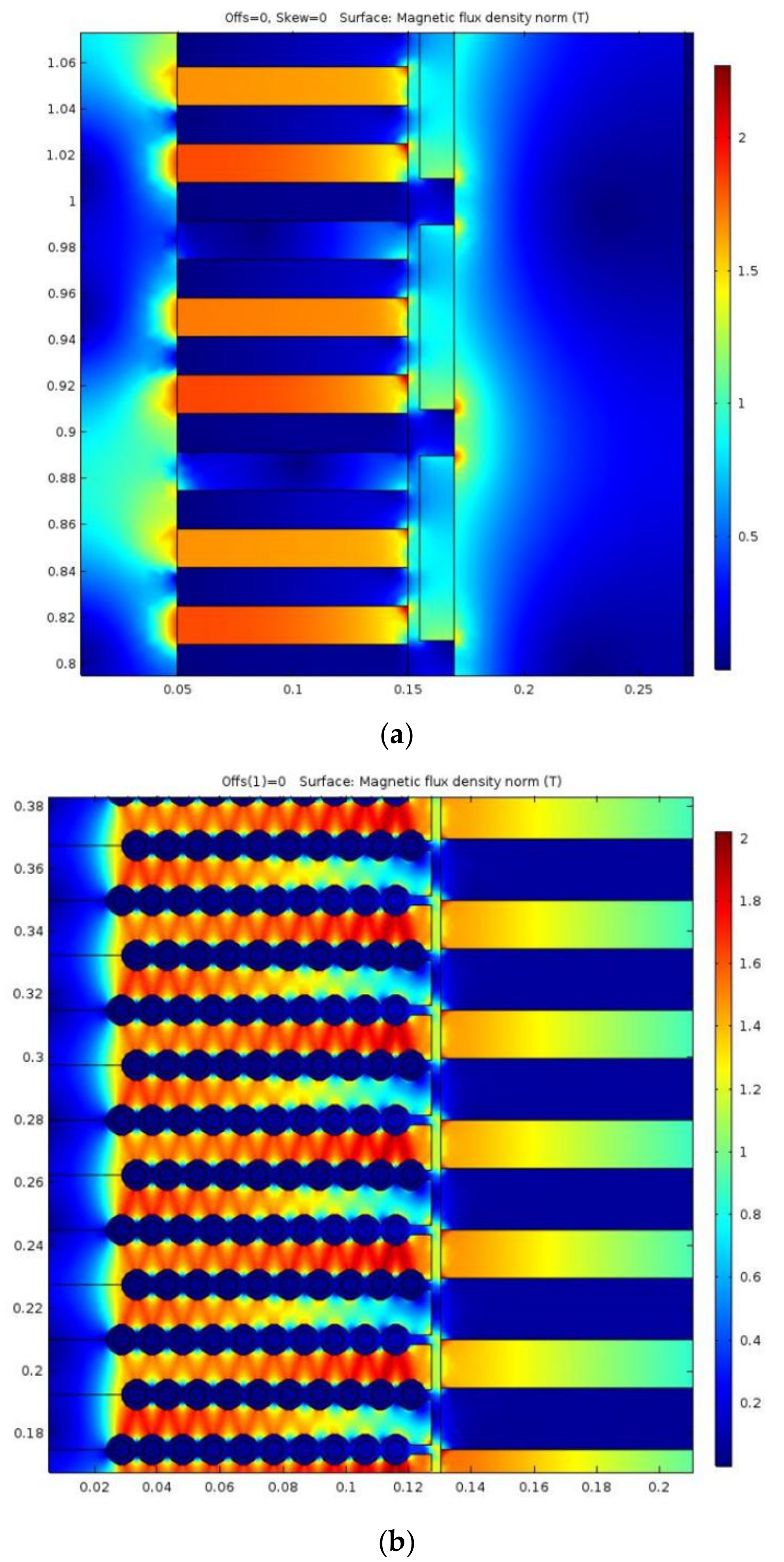To give a similar efficiency as for the ferrite generator, this machine is also rated at 2.5 A/mm² here. The machine is skewed in the same way as for machine A. A FEM simulation for machine B is shown in Figure 11a.

Machine C is simulated in 2D with a height of 30 poles, where the pole length is 35 mm. The same translator width as in machine A was used in the 2D simulation, which is probably larger than in their 3D design, which will give a heavier and more expensive translator. Also, this is the first ferrite prototype that they built, which may now be obsolete. Machine C has a very different stator than the machines A and B, and is composed of three parallel single phase sections to form a three phase machine [8]. A noticeable difference is also that this machine is cable wound, which gives a lower slot fill factor. All of the parameters for the geometry of machine C has not been found, but has been estimated from images in [8], and the simulation results found seem to be consistent with the concept. The end windings are assumed to add 20% extra length of the winding, which is less than for machines A and B due to the short pole length. The current density used has been estimated to 1.5 A/mm², which seems to be consistent with their power rating of around 30 kW at 0.7 m/s. This current density has been used in the comparison. As for machine A, which is the other ferrite machine, saturation effects are important for machine C and increasing the current density to 2.5 A/mm² only increases the shear stress from 9 to 13 N/mm², which is considerably less than expected from simple circuit theory. In the economic analysis that is made here, it would still be beneficial, although there might be a thermal current limit on the cables that prevent this. The efficiency would drop to 70.0%, but the material costs would drop by a factor 9/13, which also approximately yields for the clamping force and magnetic stiffness factors. In Table 3, the cost for the losses would increase with 76 €/kN, but the material cost per kN would decrease with 299 €/kN, giving a total cost reduction of 223 €/kN or 13.2% in Table 3. The reason why this could pay off is that the relatively large iron and friction losses is largely unaffected by the current, reducing them by a factor 9/13 per kN, which then counteracts the increase in copper losses and it limits the total efficiency reduction to 2.9%. A FEM simulation for machine C is shown in Figure 11b.

Machine D is the first prototype machine of transverse flux type being developed and built by the author, which is presented in [18,19]. The performance and active mass for this machine is simply taken from that design, with slight modifications that has been made after this publication. The prototype will now be built of half this size, 100 kN, due to lack of time. This machine looks like a three phase transformer, with aluminum winding and grain-oriented steel in the transformer core. It is of transverse flux type, but it does actually not have a transverse magnetic flux. In this machine, six airgaps are magnetically connected in series, which reduces the amount of iron in the stator and translator. Although grain-oriented steel is more expensive than non-oriented steel, there is no spill while building the transformer core and the cost for the stator steel is assumed to be the same as for the other machines. Neodymium magnets are placed in the stator, and the translator only contains iron and structure material. Thereby, all of the magnets are used all the time, which lowers the magnet cost. A drawback with machine D is that the power factor is only 0.5, which will increase the cost of the converter and the associated converter losses. Since the first prototype of this machine is currently under construction, the simulations have not yet been experimentally verified. The numbers that are presented here indicate that it will grossly outperform the other machines, both on efficiency, force density, and cost, but it should be remembered that the generator is not yet built and that a number of mechanical tricks have to be employed to maintain the 1 mm airgap that is required for the machine to perform this well. It is therefore a great challenge to develop and build such a machine, considerably more challenging than for machines A–C, which is a drawback for machine D that should be seriously taken into regard. Thereby, it does not disqualify the other concepts, at least not yet. Images of FEM simulations are given in [19].

The demagnetization of ferrite magnets will slightly lower the performance for machines A and C. This has not been regarded in the comparison.

3. Discussion

In the optimization and in machine A and C, the width $w_T=0.2 \mathrm{m}$ has been used for the translator, which is rather broad. A double-sided or multisided symmetric approach is the most likely solution, since the attraction forces from the stator on the translator then ideally cancel by symmetry. With such a solution, the width $w_T$ is likely to be smaller to save some material, and then the optimal pole length becomes a bit shorter. 3D effects will also affect the optimal pole length. However, it is evident that the optimal pole length for typical slow speed ferrite magnet machines is in the range of 7–15 cm, unless the airgap is very small (see Figure 3), and that the choice of pole length is very important for the performance of slow speed ferrite magnet generators although the optimum is flat. Also note here that the iron losses can be very large, potentially over 10%, as predicted for machine C, if the pole length is chosen too short. This is since the lower shear stress will increase the amount of iron magnetized per kN and since the iron losses are approximately proportional to frequency at low frequencies. Note also that the iron losses are mainly independent on the stator current, and thereby becomes a larger fraction of the power at partial current load in contrast to the copper losses that becomes a smaller fraction of the total power at partial current load. The iron losses in the translator are expected to be very small if the iron is laminated, since the flux density in these parts only varies with a small amplitude, except at the teeth. The optimization shows that if the airgap is sufficiently small, 3 mm or less, an average airgap magnetic flux density of 0.8–0.9 T can be reached, which indicates that similar shear stresses as with surface mounted neodymium magnets can be reached. The shear stress in the generator that is presented here is only slightly lower than in the work by Polinder et al. [9,10], and the cost per kN of these machines seem to be similar. The demagnetization effects slightly lower the performance of machine A, and sets some requirements on the magnet grade used. It seems that a ferrite generator similar to machine A can be a fully viable alternative to classical neodymium magnet generators for wave power, especially if the neodymium magnet price would increase. However, although the magnets are available at a very low cost, linear ferrite magnet generators for wave power applications has several drawbacks when compared to neodymium magnet generators that should be taken into regard:

• The demagnetization needs to be carefully regarded in the design, and the choice of magnet grade may be crucial for performance. Demagnetization from the current loading and fault cases should be analyzed, as well as demagnetization effects from sheer geometry choices.
• The linear bearings, which are a rather expensive part of the machine, could potentially experience several times larger normal forces with a ferrite solution when compared to a surface mounted neodymium magnet solution and need to be dimensioned for them. This will add to cost.
• The translator will be heavier, which may or may not be a drawback.

Although the ferrite magnet technology for generators has been known for decades, it seems that the results that are presented here are not well known to the wave power community and the findings here may therefore be rather important. The comparison between machines A and C strongly indicates that there are great opportunities to cut costs for the concept that was described in [8] by increasing the pole length. The shear stress in [8] is not given, but it is calculated to around 9 kN/m² from the simulations. Machine A is made of the same materials as machine C, and it has a calculated shear stress of 42 kN/m², which indicates that the force density can be increased by a factor of 4 or so if the pole length is increased four times and the stator layout is modified. This would reduce the cost and size of the machine. Also, this would reduce the iron losses in the machine grossly and relax the demagnetization of the ferrite magnets, which possibly enables the use of other magnet grades.

It is popular to form linear wave power generators into a tubular shape, instead of using a flat structure. This is beneficial in some aspects, and it can reduce the end windings grossly. Such a concept is presented in [25]. A mechanical analysis, where the structure and the bearing system are designed, is however required to determine if this could improve the concept or not.

Machine D, which is shown in the comparison, illustrates the strength of the transverse flux type machines for low speed applications, where so-called magnetic gearing solves the low-speed problem of high copper losses and increases the force density. The future will tell whether these machines could reach maturity and outcompete the more standard types of generators analyzed here. If so, the levelized cost of energy for wave power devices could be reduced significantly.

4. Materials and Methods

The numerical calculations in this text have been made using Comsol Multiphysics 5.2 (COMSOL, Stockholm, Sweden). A generic iron similar to M470-50A has been used with unity stacking factor as non-linear iron. The skewing has been performed by calculating 21 different skewed positions and calculating the average values of force and flux in MATLAB (R2015a, The MathWorks, Inc., Natick, MA, USA). Only static simulations have been made, and 61 discrete steps with sinusoidal currents were used in Section 2.4 and Section 2.5 over one pole length displacement. The voltage was generally calculated assuming a speed of 1 m/s.

5. Conclusions

In this text, the translator geometry for linear ferrite magnet generators with the application of wave power has been examined and optimized for the extremely low speeds that are involved in wave power, around 1 m/s or even less. An analytical expression for the optimal pole length has been derived, where it has been found that, for typical values, the pole length should be around 7–15 cm for airgaps of 3 mm where it is emphasized that the choice of pole length is very important for the performance of the generator. With a proper pole length and an airgap of 3 mm or less, it seems fully possible to achieve similar shear stresses as in the case with surface mounted neodymium magnets. Demagnetization effects are also examined, and it is evident that the demagnetization effects must carefully be taken into regard in the design, where especially the mounting process needs to be examined carefully. Failure to do so may lower the performance of the machine significantly. Finally, an example machine is designed and analyzed, in order to illustrate that reasonable shear stresses can be achieved at these low speeds. This machine is compared to three other concepts, showing that it is competitive to neodymium generator counterparts. Future analysis should be focused on demagnetization studies and optimization of k, as well as structural design and bearing design, where different geometrical layouts should be investigated and evaluated from a cost perspective. 3D effects should also be considered.

References

1. Gunn, K.; Stock-Williams, C. Quantifying the wave power resource. Renew. Energy 2012, 44, 296–304. [Google Scholar] [CrossRef]
2. Binns, K.J.; Kurdali, A. Permanent-magnet ac generators. In Proceedings of the Institution of Electrical Engineers; IET Digital Library: London, UK, 1979; pp. 690–696. [Google Scholar]
3. Chen, Z.; Spooner, E. A modular, permanent-magnet generator for variable speed wind turbines. In Proceedings of the 1995 Seventh International Conference on Electrical Machines and Drives, Durham, UK, 11–13 September 1995; IET: Stevenage, UK, 1995. [Google Scholar]
4. Spooner, E.; Williamson, A.C. Direct coupled, permanent magnet generators for wind turbine applications. IEE Proc.-Electr. Power Appl. 1996, 143, 1–8. [Google Scholar] [CrossRef]
5. Spooner, E.; Williamson, A.C.; Catto, G. Modular design of permanent-magnet generators for wind turbines. IEE Proc.-Electr. Power Appl. 1996, 143, 388–395. [Google Scholar] [CrossRef]
6. Muljadi, E.; Butterfield, C.P.; Wan, Y.-H. Axial-flux modular permanent-magnet generator with a toroidal winding for wind-turbine applications. IEEE Trans. Ind. Appl. 1999, 35, 831–836. [Google Scholar] [CrossRef]
7. Dubois, M.R.; Polinder, H.; Ferreira, J.A. Comparison of generator topologies for direct-drive wind turbines. In Proceedings of the 2000 IEEE Nordic Workshop on Power and Industrial Electronics, Aalborg, Denmark, 13–16 June 2000; pp. 22–26. [Google Scholar]
8. Ekergård, B. Full Scale Applications of Permanent Magnet Electromagnetic Energy Converters: From Nd2Fe14B to Ferrite. Ph.D. Thesis, Uppsala University, Uppsala, Sweden, 2013. [Google Scholar]
9. Polinder, H.; Damen, M.E.; Gardner, F. Linear PM generator system for wave energy conversion in the AWS. IEEE Trans. Energy Convers. 2004, 19, 583–589. [Google Scholar] [CrossRef]
10. Polinder, H.; Mecrow, B.C.; Jack, A.G.; Dickinson, P.G.; Mueller, M.A. Conventional and TFPM linear generators for direct-drive wave energy conversion. IEEE Trans. Energy Convers. 2005, 20, 260–267. [Google Scholar] [CrossRef]
11. Mueller, M.A.; Xiang, J.; Baker, N.J.; Brooking, P.R.M. Dynamic Modeling of a Linear Vernier Hybrid Permanent Magnet Machine Coupled to a Wave Energy Emulator Test Rig. In Recent Developments of Electrical Drives; Springer: Dordrecht, The Netherlands, 2006; pp. 39–49. [Google Scholar]
12. Baker, N.J.; Spooner, E.; Mueller, M.A. Permanent magnet air-cored tubular linear generator for marine energy converters. In Proceedings of the 2004 Second International Conference on Power Electronics, Machines and Drives, Edinburgh, UK, 31 March–2 April 2004. [Google Scholar]
13. Hodgins, N.; Keysan, O.; McDonald, A.S.; Mueller, M.A. Design and testing of a linear generator for wave-energy applications. IEEE Trans. Ind. Electr. 2012, 59, 2094–2103. [Google Scholar] [CrossRef]
14. Leijon, M.; Bernhoff, H.; Agren, O.; Isberg, J.; Sundberg, J.; Berg, M.; Karlsson, K.E.; Wolfbrandt, A. Multiphysics simulation of wave energy to electric energy conversion by permanent magnet linear generator. IEEE Trans. Energy Convers. 2005, 20, 219–224. [Google Scholar] [CrossRef]
15. Prudell, J.; Stoddard, M.; Amon, E.; Brekken, T.K.; Von Jouanne, A. A permanent-magnet tubular linear generator for ocean wave energy conversion. IEEE Trans. Ind. Appl. 2010, 46, 2392–2400. [Google Scholar] [CrossRef]
16. Huang, L.; Yu, H.; Hu, M.; Zhao, J.; Cheng, Z. A novel flux-switching permanent-magnet linear generator for wave energy extraction application. IEEE Trans. Magn. 2011, 47, 1034–1037. [Google Scholar] [CrossRef]
17. Du, Y.; Chau, K.T.; Cheng, M.; Wang, Y. A linear magnetic-geared permanent magnet machine for wave energy generation. In Proceedings of the 2010 International Conference on Electrical Machines and Systems (ICEMS), Incheon, Korea, 10–13 October 2010; IEEE: Piscataway, NJ, USA, 2010. [Google Scholar]
18. Hagnestål, A. A low cost and highly efficient TFM generator for wave power. In Proceedings of the 2006 3rd Asian Wave and Tidal Energy Conference (AWTEC), Singapore, 24–28 October 2016; pp. 822–828. [Google Scholar]
19. Hagnestål, A. A highly efficient and low-cost linear TFM generator for wave power. In Proceedings of the 2017 EWTEC 12th European Wave and Tidal Energy Conference, Cork, Ireland, 27 August–1 September 2017. [Google Scholar]
20. Polinder, H.; Mueller, M.A.; Scuotto, M.; de Sousa Prado, G.M. Linear generator systems for wave energy conversion. In Proceedings of the 7th European Wave and Tidal Energy Conference, Porto, Portugal, 11–14 September 2007. [Google Scholar]
21. Krause, P.; Wasynczuk, O.; Sudhoff, S.D.; Pekarek, S. Analysis of Electric Machinery and Drive Systems; John Wiley & Sons: Hoboken, NJ, USA, 2013; Volume 75, pp. 628–629. [Google Scholar]
22. Ulvgård, L. Wave Energy Converters: An Experimental Approach to Onshore testing, Deployments and Offshore Monitoring. Ph.D. Thesis, Acta Universitatis Upsaliensis, Uppsala, Sweden, 2017. [Google Scholar]
23. Frost, A.E.; Ulvgård, L.; Sjökvist, L.; Eriksson, S.; Leijon, M. Partial Stator Overlap in a Linear Generator for Wave Power: An Experimental Study. J. Mar. Sci. Eng. 2017, 5, 53. [Google Scholar] [CrossRef]
24. Polinder, H.; Mecrow, B.C.; Jack, A.G.; Dickinson, P.; Mueller, M.A. Linear generators for direct-drive wave energy conversion. In Proceedings of the 2003 IEEE International Electric Machines and Drives Conference, Madison, WI, USA, 1–4 June 2003; IEEE: Piscataway, NJ, USA, 2003; Volume 2, pp. 798–804. [Google Scholar]
25. Trapanese, M.; Cipriani, G.; Corpora, M.; Di Dio, V. A general comparison between various types of linear generators for wave energy conversion. In Proceedings of the 2017 OCEANS–Anchorage, Anchorage, AK, USA, 18–21 September 2017; IEEE: Piscataway, NJ, USA, 2017; pp. 1–5. [Google Scholar]
Figure 1. A section of a cross section of a simplified linear generator is shown, where the two-dimensional (2D) magnetic circuit that is used to calculate the flux at direct position is drawn. The dashed lines are symmetry lines that mark the boundaries of the magnetic circuit. Ferrite magnets are in light grey, iron is in dark grey, and air is in white.
Energies 11 01356 g001
Figure 2. The dependence on pole length (a) and k (b) for the magnetic flux density in the airgap in direct position in black and the average airgap flux density in red is shown for a linear generator with parameters δ = 0.003 m, wT = 0.2 m, and δr,m = 1.1. In (a), k = 0.45 and in (b), lp = 0.103 m. Values from analytical calculations, 2D Finite Element Analysis (FEA) simulations with ideal iron and 2D FEA simulations with an iron with saturation effects are shown.
Energies 11 01356 g002
Figure 3. Contour plots of the optimal pole length from Equation (14) vs. δ and w T (a), and contour plots of B a from (13) vs. l p and w T (b). Values k = 0.45 and μ r , m = 1.1 are used, and in (b) δ = 0.003   m .
Energies 11 01356 g003
Figure 4. Demagnetization curves for ferrite magnet grades for the ferrite magnet manufacturer Spacemagnets. (a) HTY45E; (b) HTY40N.
Energies 11 01356 g004
Figure 5. The magnetic flux density inside the magnets for a linear generator, when the translator is inside the stator (a) and outside the stator (b). The values are from 2D simulations with k = 0.45, δ′ = 0.003 m, wT = 0.2 m, and μr,m, and the stator is simplified.
Energies 11 01356 g005
Figure 6. The Bz component is calculated for a step in the in the mounting process of a square translator block of Y40 ferrite magnets and iron parts, where a layer of magnets is on the top surface. Results from 2D and three-dimensional (3D) simulations at the center of the top surface of the top magnet for different pole lengths is given in (a) and (b) shows the special case of 35 mm pole length in 3D. Calculations are made using the parameters k = 0.45, wT = 0.2 m, and μr,m = 1.1. The 3D simulations assume a stacking width ls = 0.2 m, which improves the demagnetization situation for the magnets when compared to the 2D case to some extent but also reduces the magnetic flux density in the airgap.
Energies 11 01356 g006
Figure 7. Flow charts for the electromagnetic design process for the ferrite magnet generator, where (a) takes demagnetization effects into regard and (b) does not.
Energies 11 01356 g007
Figure 8. A cross section of the layout of the ferrite generator design, where the white arrows mark the direction of magnetization for the ferrite magnets: (a) The main parts of the generator; and, (b) The winding of the phases.
Energies 11 01356 g008
Figure 9. The magnetic flux density modulus for the example generator at 2.5 A.
Energies 11 01356 g009
Figure 10. Characteristics of the generator both for the skewed and the non-skewed case for no-load and a current density of 2.5 A: (a) The damping force vs. position over one pole length; (b) The average damping force over one pole vs. current; (c) The flux linkage vs. position over one pole length; and, (d) The voltage vs. position over one pole length, where the no-load voltage is trapezoidal rather than sinusoidal.
Energies 11 01356 g010aEnergies 11 01356 g010b
Figure 11. FEA calculations for two of the reference machines: (a) Machine B, the neodymium magnet generator made by Polinder et al., simulated with a current rating of 2.5 A/mm2; and, (b) Machine C, the ferrite generator designed and built by the Uppsala group, simulated with a current rating of 1.5 A/mm2.
Energies 11 01356 g011