Prediction-Learning Algorithm for Efficient Energy Consumption in Smart Buildings Based on Particle Regeneration and Velocity Boost in Particle Swarm Optimization Neural Networks

Abstract
:1. Introduction
2. Literature Review
3. Particle Swarm Optimization-Based Neural Networks (PSO-NN) Prediction Methodology
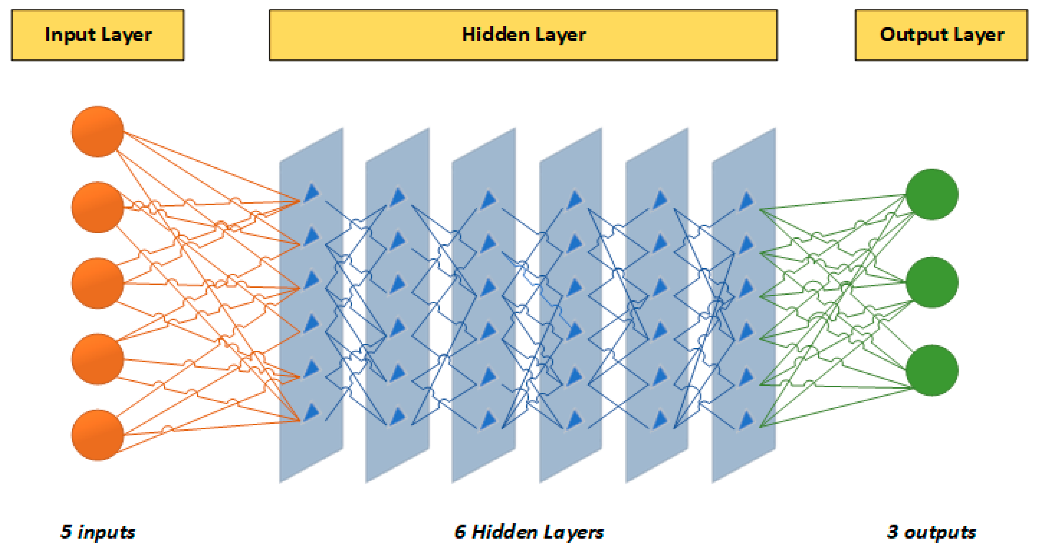
3.1. Neural Networks (NNs)
3.2. Particle Swarm Optimization (PSO)
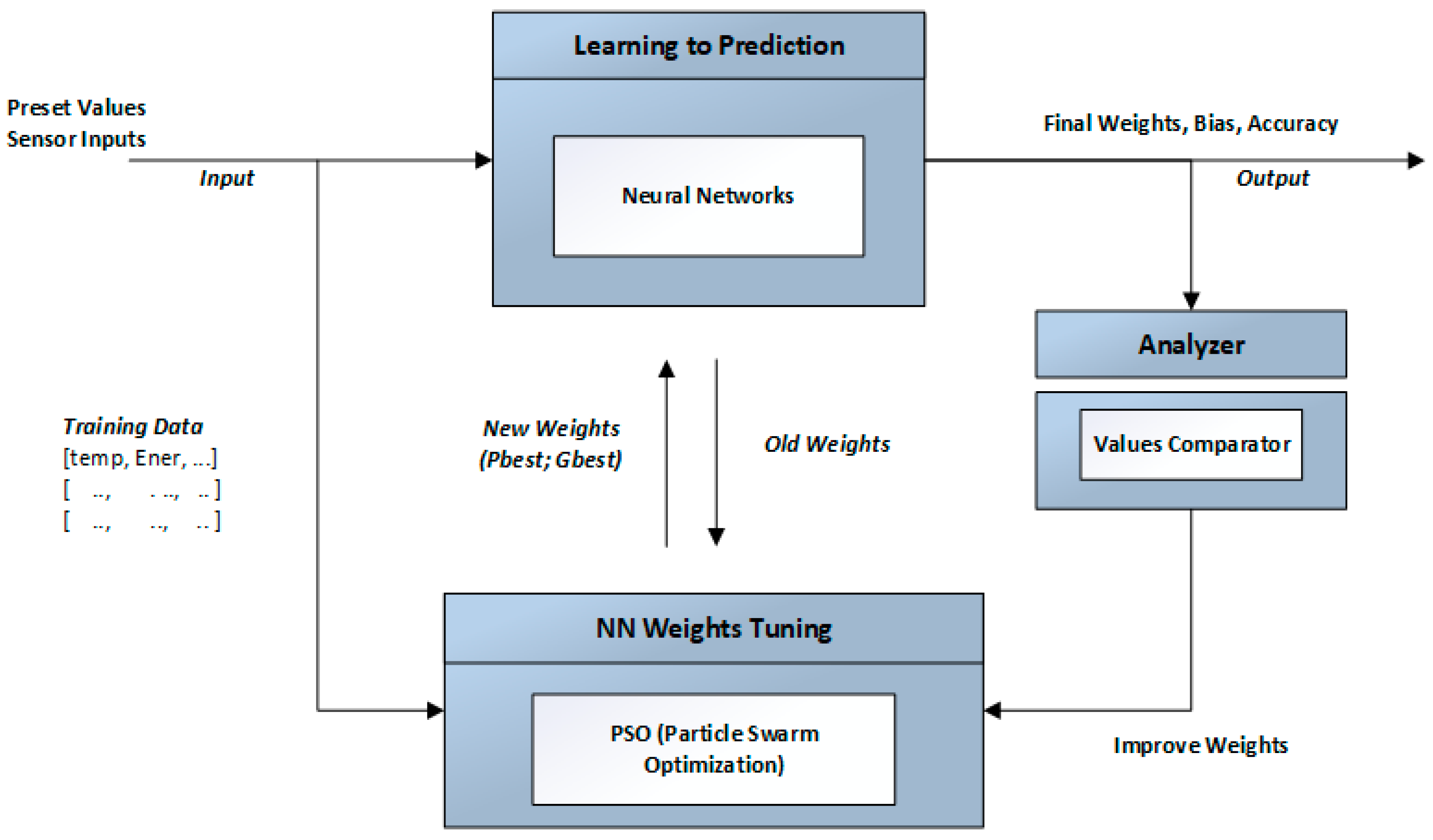
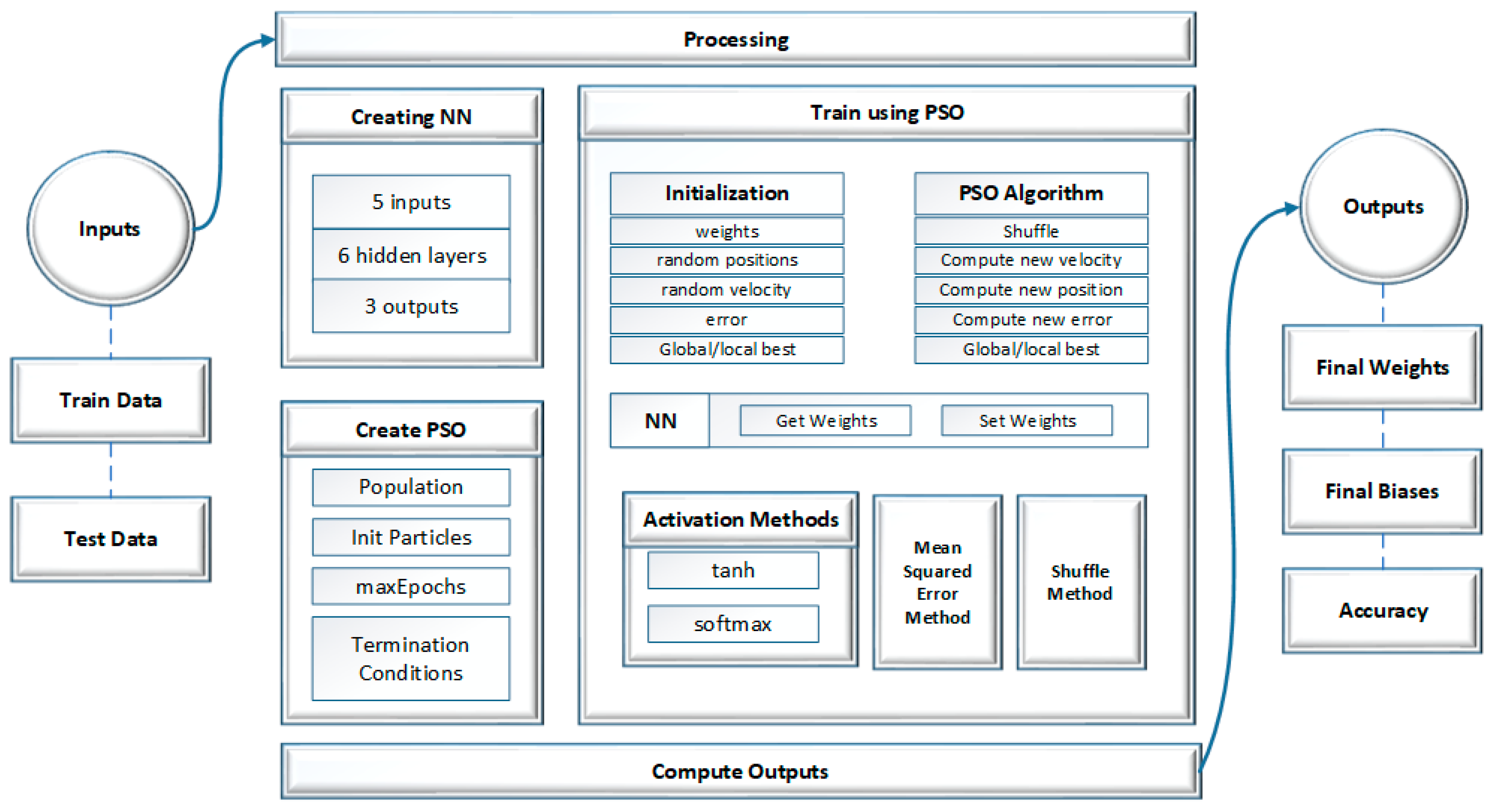
3.3. Training NNs with PSO
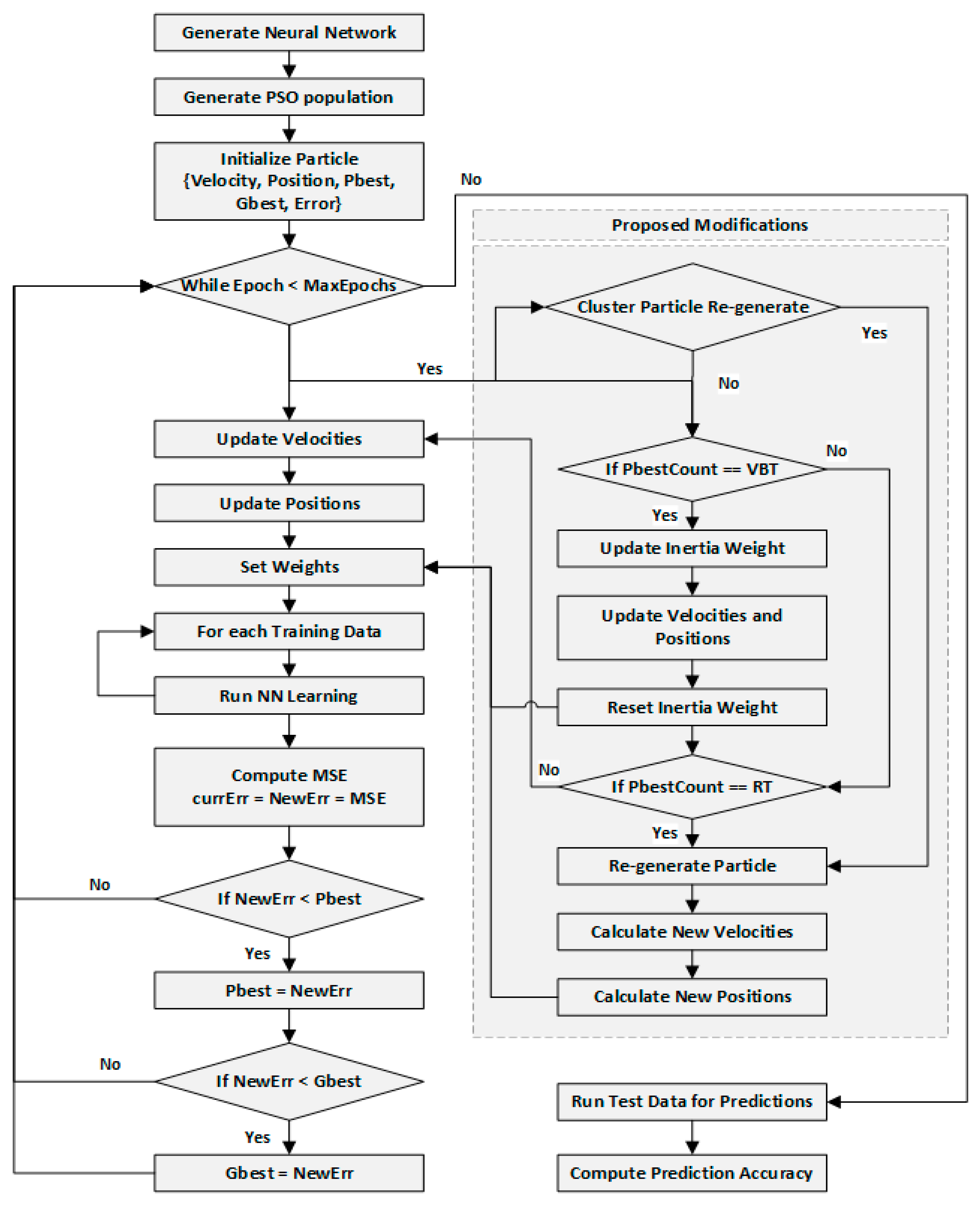
3.4. Modified PSO-NN
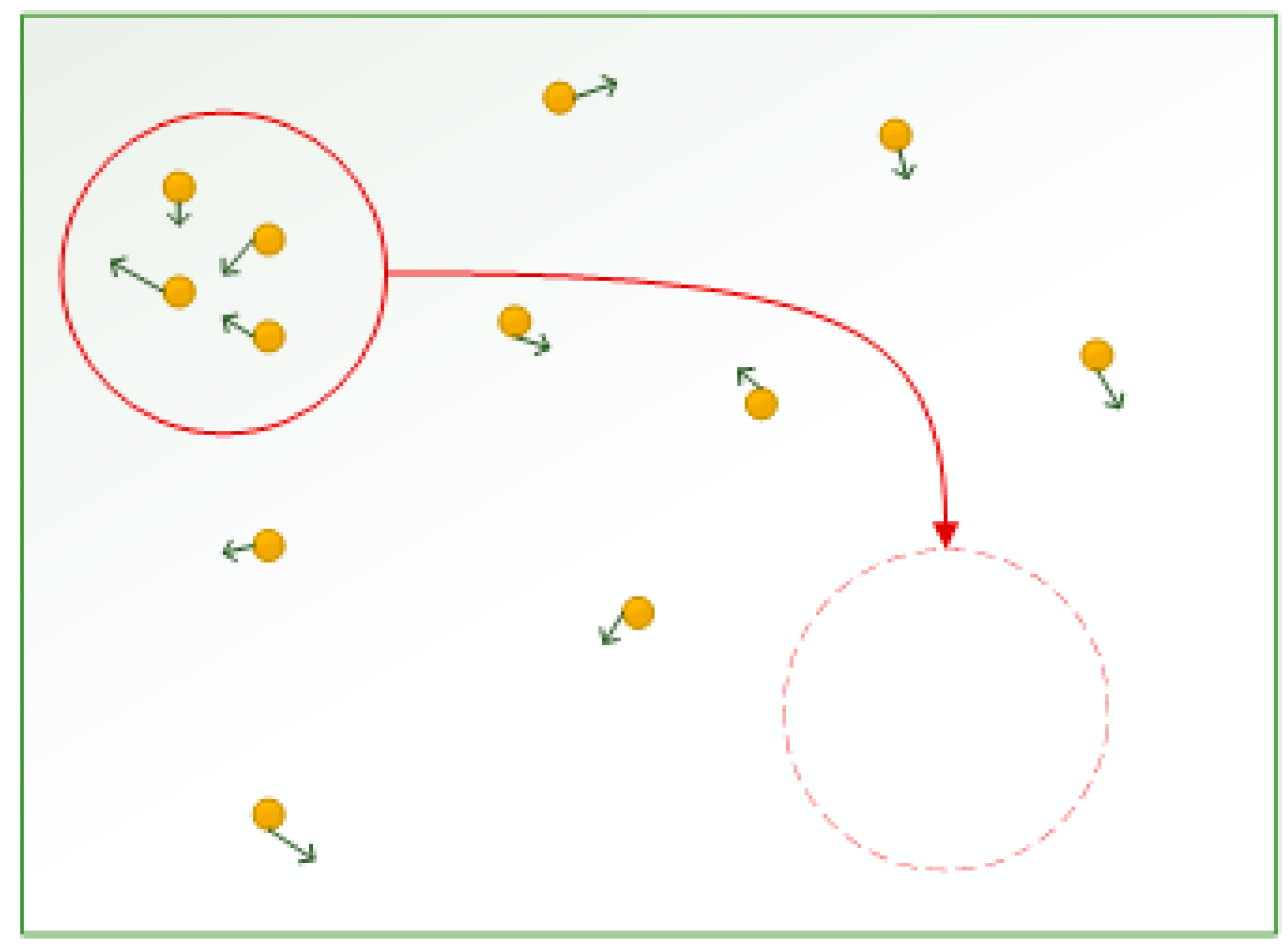
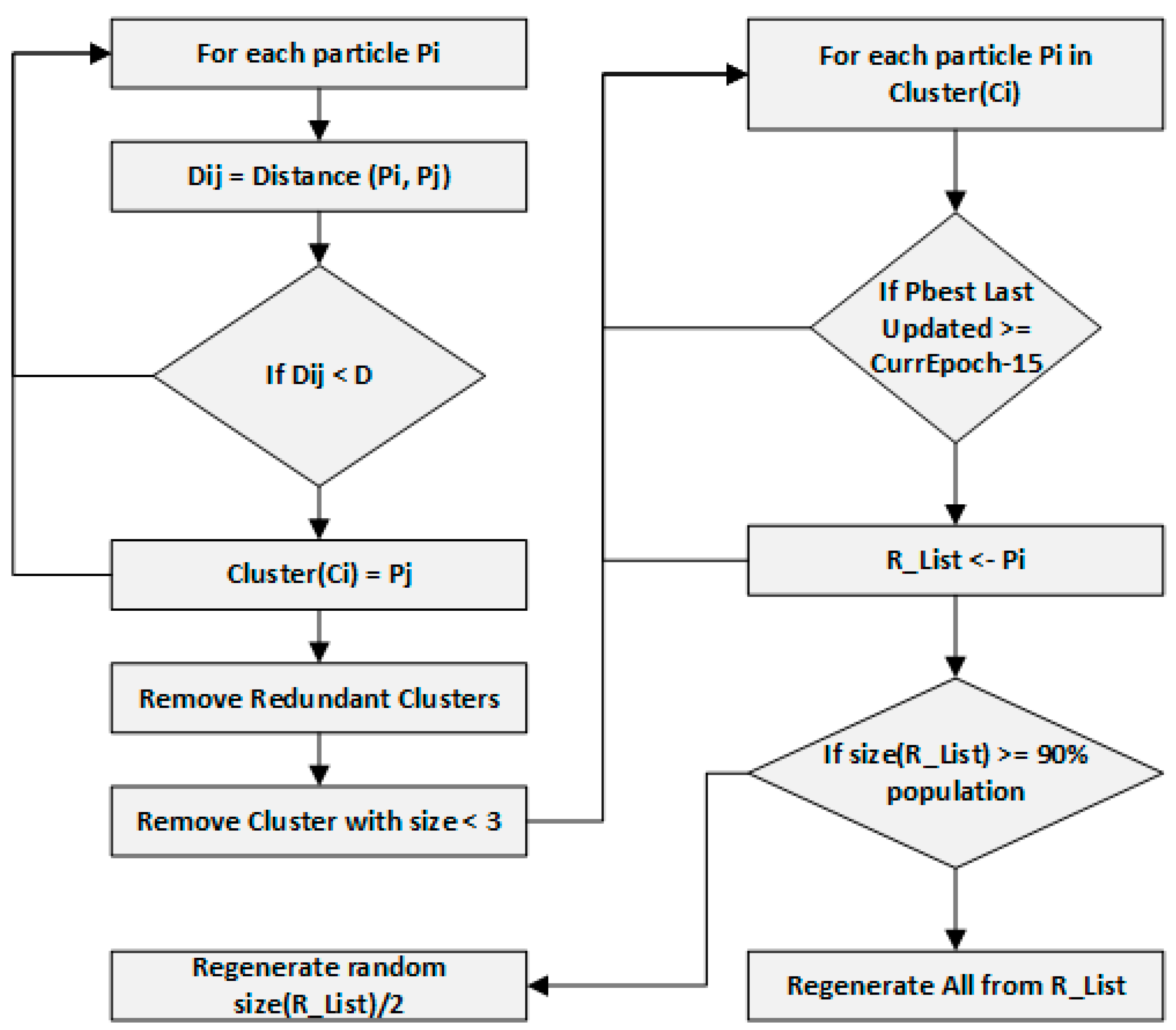
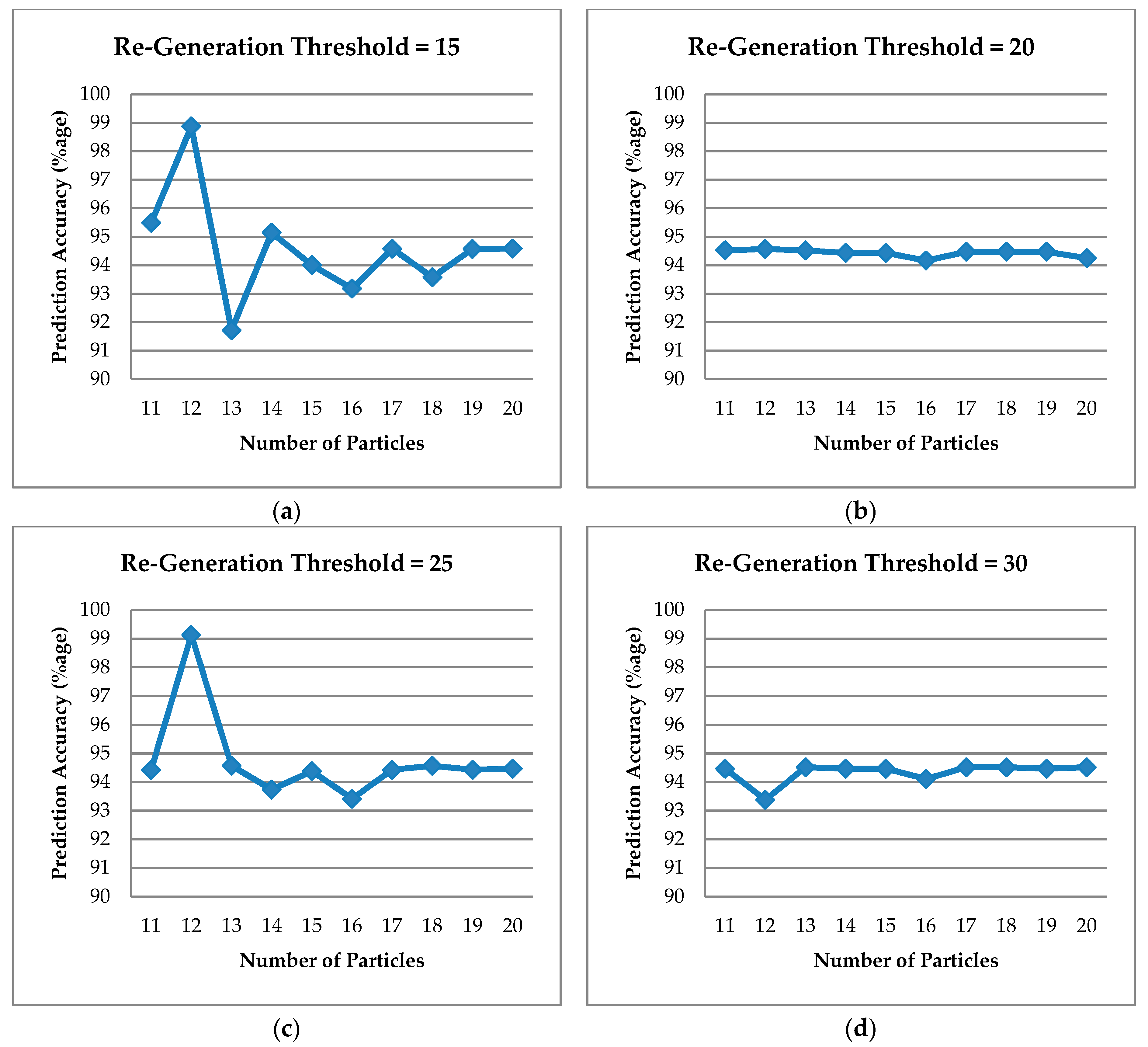
3.4.1. Re-Generation Based PSO-NN (R-PSO-NN)
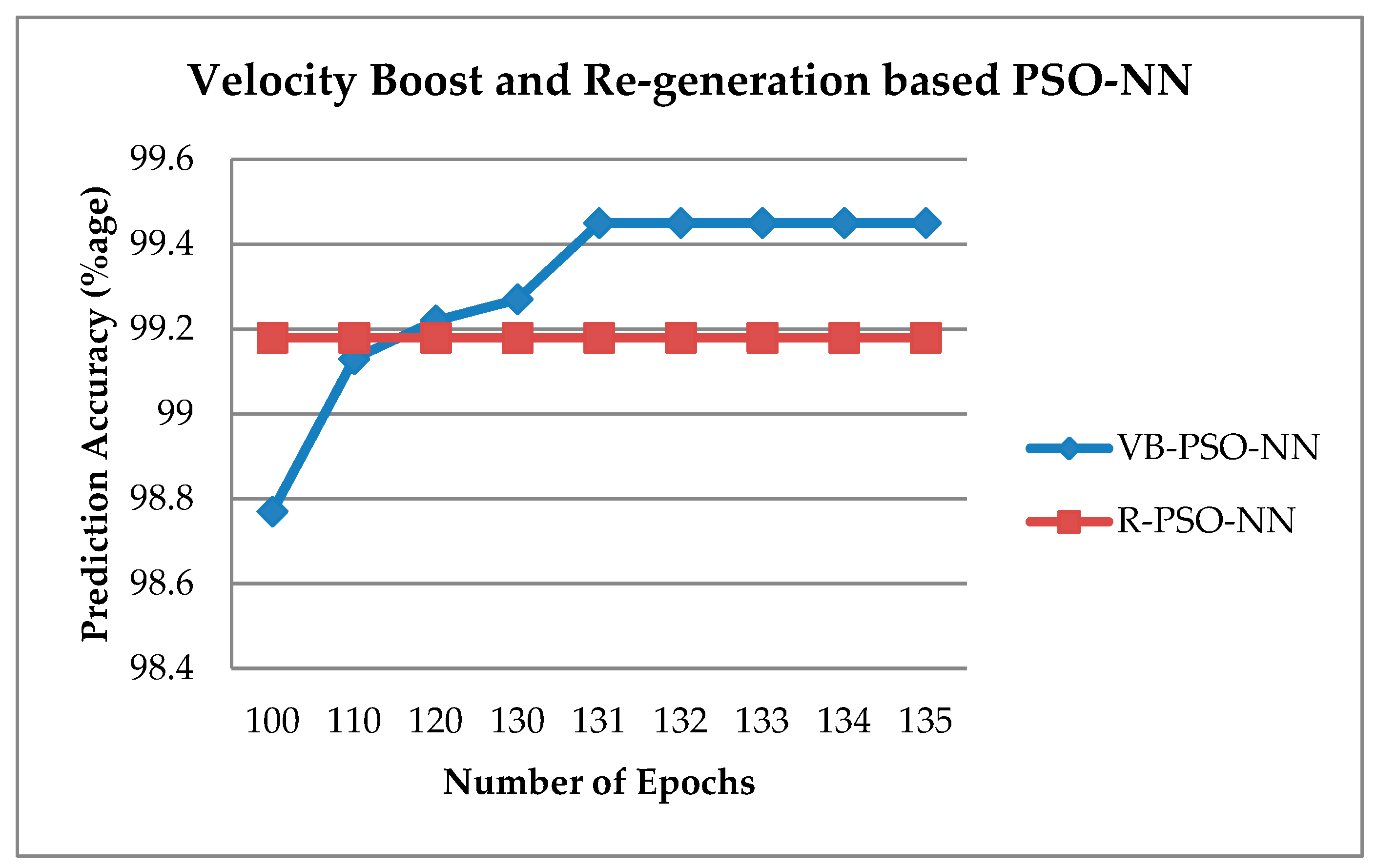
3.4.2. Velocity Boost-Based PSO-NN (VB-PSO-NN)
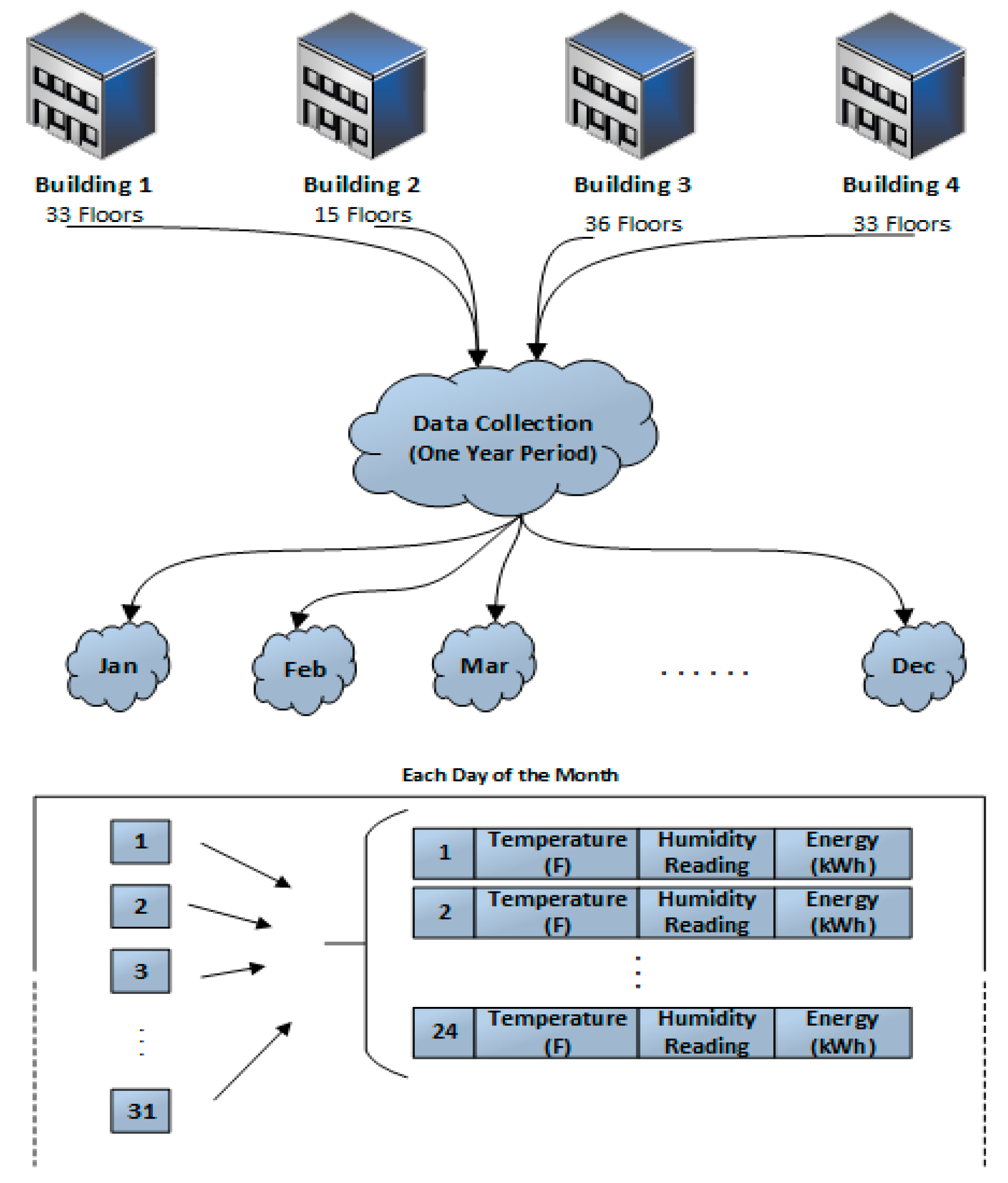
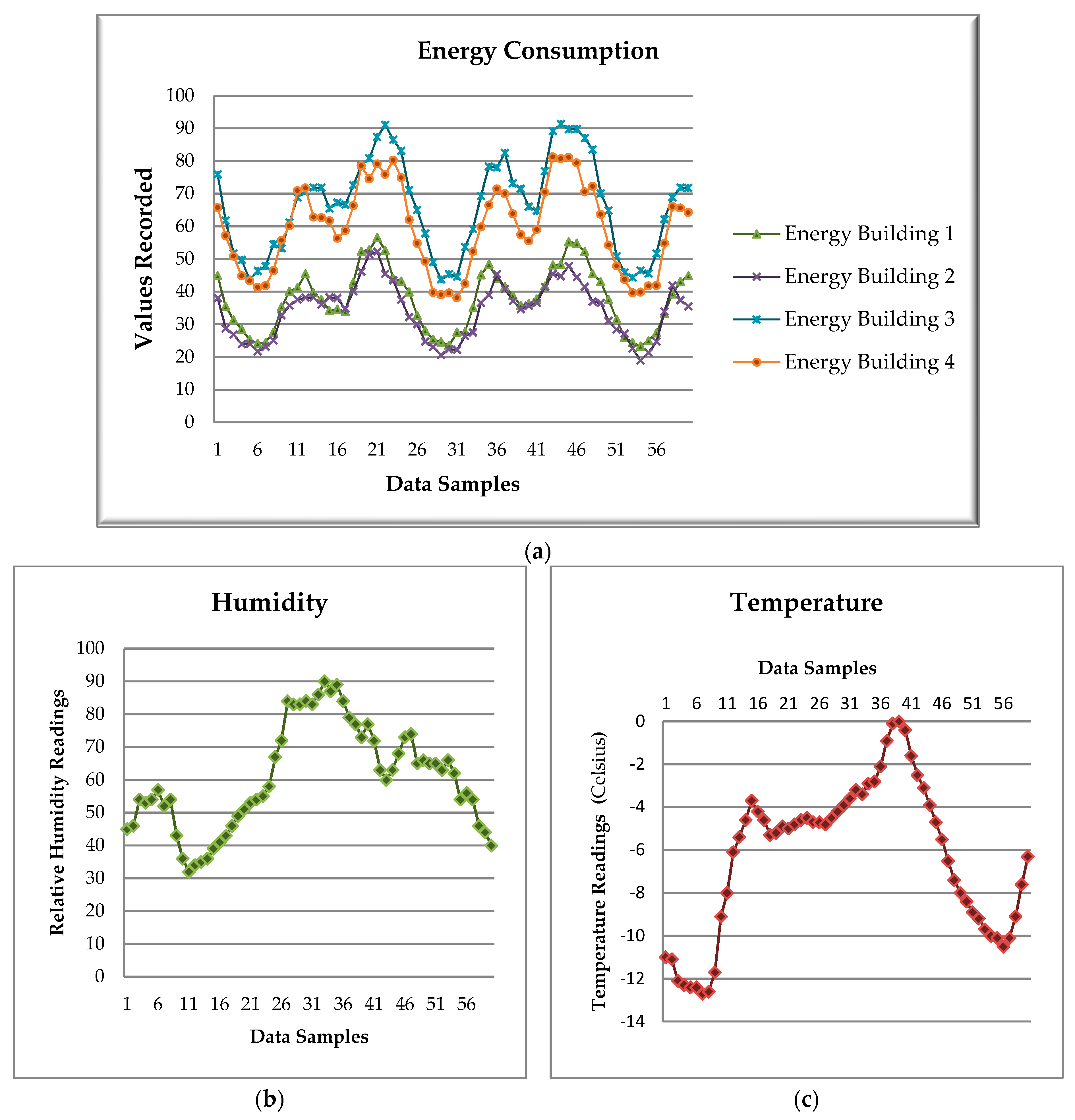
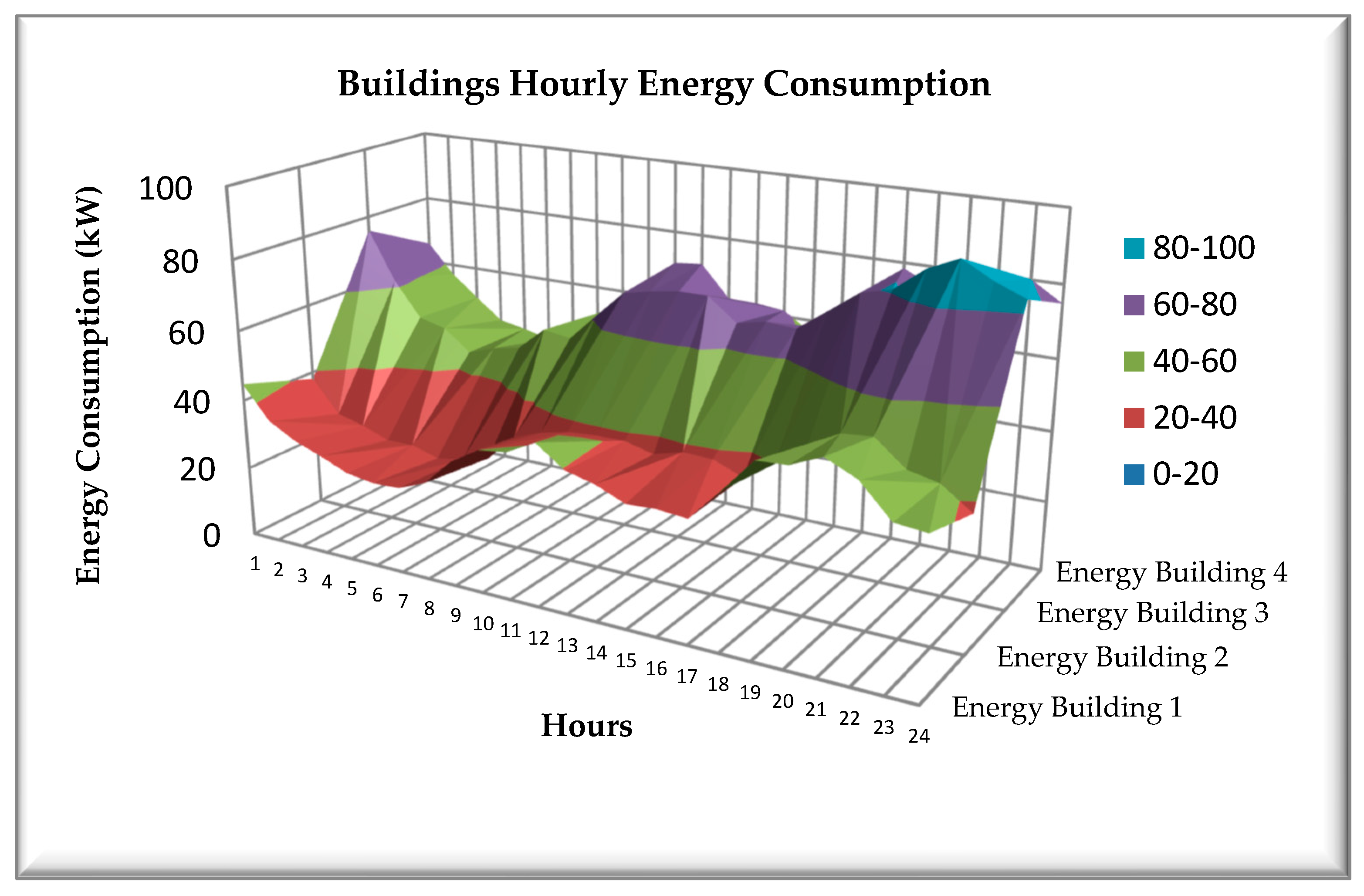
4. Data Set and Experimental Setup
4.1. Data Set
4.2. Experimental Setup
5. Results Analysis
5.1. Re-Generation Threshold (RT)
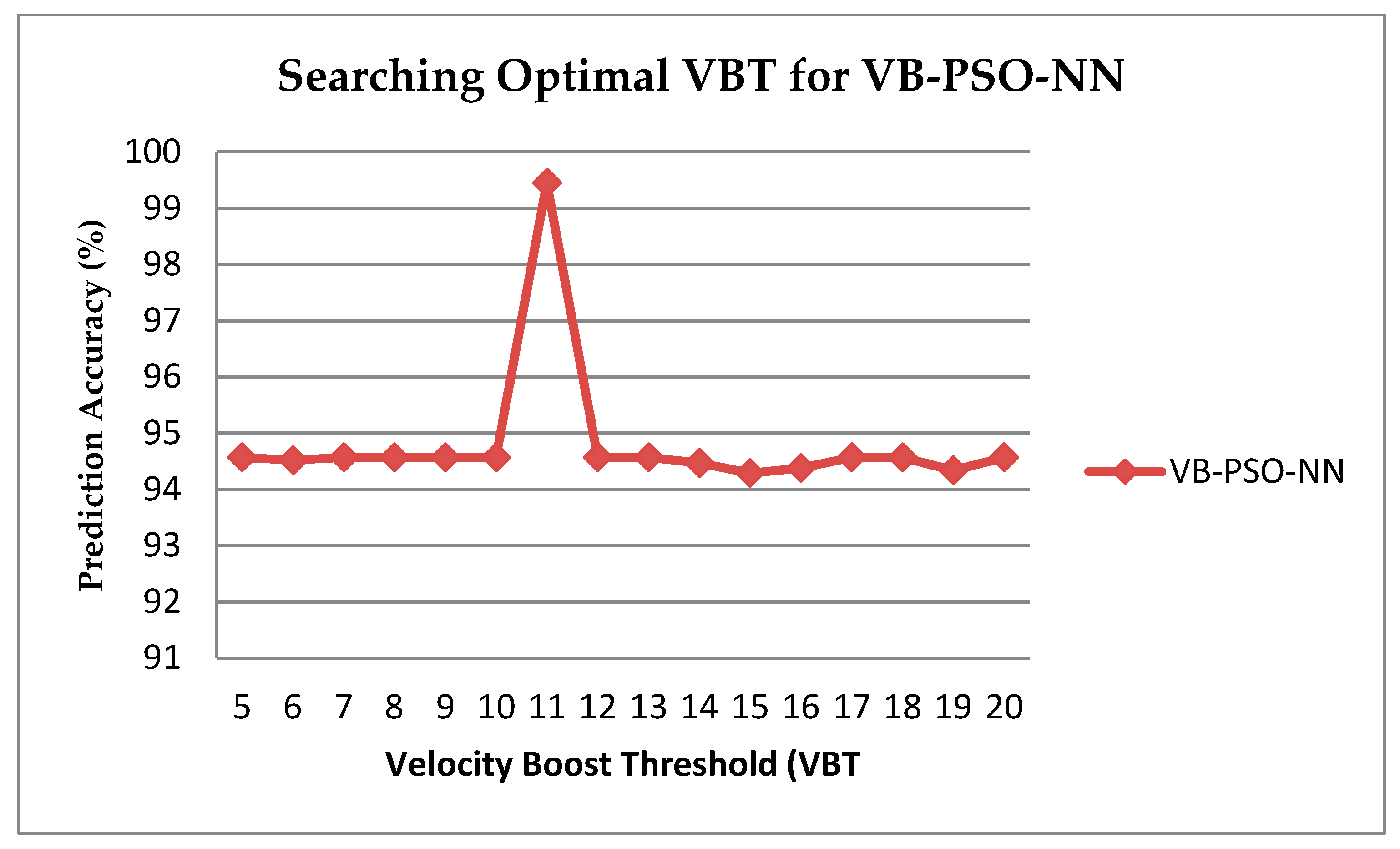
5.2. Velocity Boost Threshold (VBT)
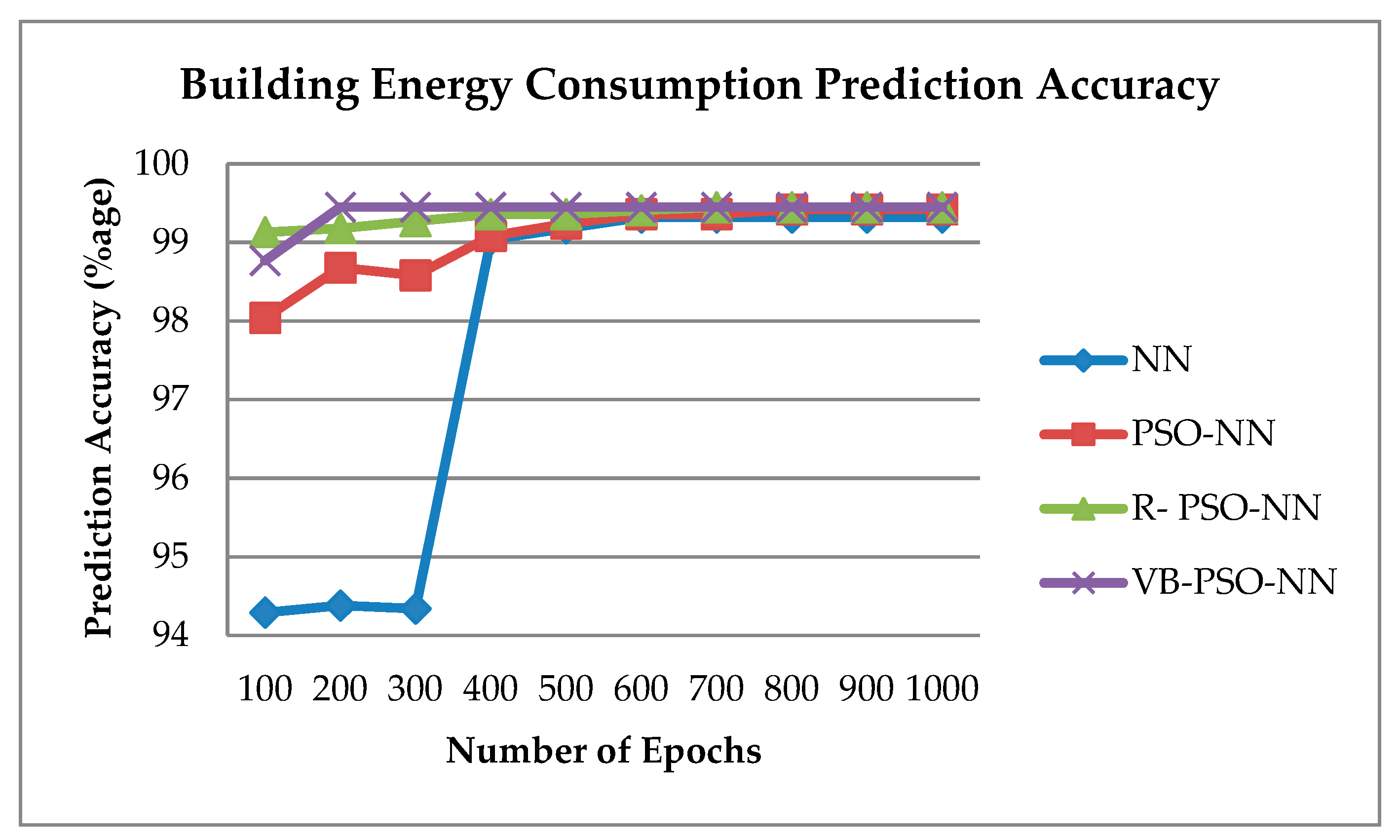
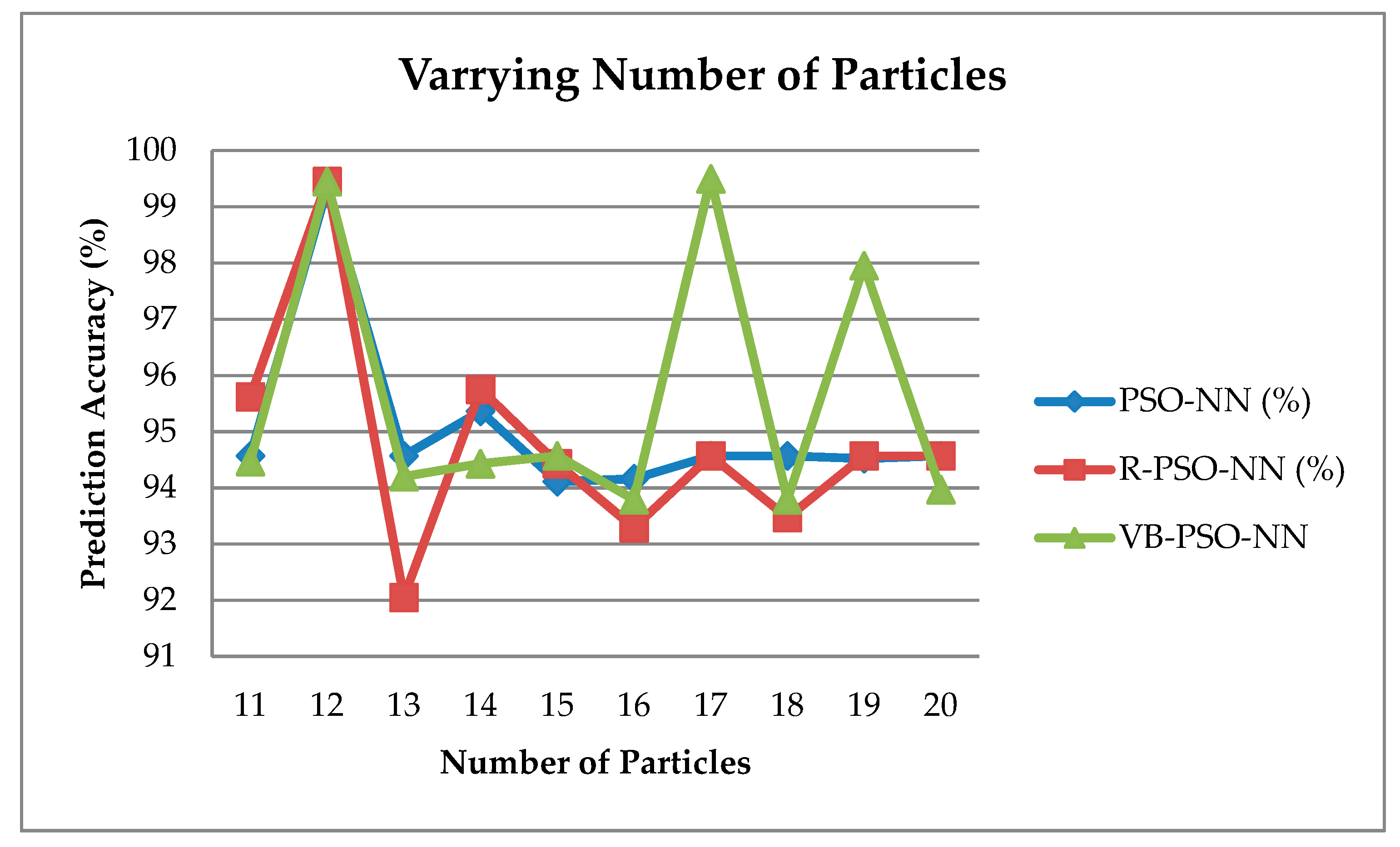
5.3. Number of Particles and Epochs Comparison
6. Discussion
7. Conclusions
Author Contributions
Acknowledgments
Conflicts of Interest
References
- Global Demand for Energy Will Peak in 2030, Says World Energy Council. Available online: https://www.theguardian.com/business/2016/oct/10/global-demand-for-energy-will-peak-in-2030-says-world-energy-council (accessed on 5 April 2018).
- Energy Information Korea. 2016. Available online: https://www.keei.re.kr/web_keei/en_publish.nsf/XML_Portal_New/B9C4089854585599492580BF0009503E/$file/EnergyInfo2016.pdf (accessed on 4 May 2018).
- International Energy Outlook. 2017. Available online: https://www.eia.gov/outlooks/ieo/pdf/0484(2017).pdf (accessed on 5 April 2018).
- Deru, M.; Torcellini, P. Source Energy and Emission Factors for Energy Use in Buildings (Revised); No. NREL/TP-550-38617; National Renewable Energy Laboratory (NREL): Golden, CO, USA, 2007.
- The Internet of Things: Making the Most of the Second Digital Revolution. Available online: https://www.gov.uk/government/uploads/system/uploads/attachment_data/file/409774/14-1230-internet-of-things-review.pdf (accessed on 5 April 2018).
- Korea’s Smart Homes Need New Lessons. Available online: http://koreajoongangdaily.joins.com/news/article/article.aspx?aid=3029201 (accessed on 5 April 2018).
- Korea Energy Agency. 2014. Available online: http://www.energy.or.kr/web/kem_home_new/energy_issue/mail_vol22/pdf/publish_05_201507.pdf (accessed on 5 April 2018).
- 4 Ways the Internet of Things Is Saving Energy, Water & Money. Available online: http://dadolabs.com/energyefficiency/ (accessed on 5 April 2018).
- Amasyali, K.; El-Gohary, N. Building lighting energy consumption prediction for supporting energy data analytics. Procedia Eng. 2016, 145, 511–517. [Google Scholar] [CrossRef]
- Hu, Y.-C. Electricity consumption prediction using a neural-network-based grey forecasting approach. J. Oper. Res. Soc. 2017, 68, 1259–1264. [Google Scholar] [CrossRef]
- Israr, U.; Ahmad, R.; Kim, D. A Prediction Mechanism of Energy Consumption in Residential Buildings Using Hidden Markov Model. Energies 2018, 11, 358. [Google Scholar] [CrossRef]
- Perez-Lombard, L.; Ortiz, J.; Pout, C. A review on buildings energy consumption information. Energy Build. 2008, 40, 394–398. [Google Scholar] [CrossRef]
- Zhao, H.-X.; Magoules, F. A review on the prediction of building energy consumption. Renew. Sustain. Energy Rev. 2012, 16, 3586–3592. [Google Scholar] [CrossRef]
- Ahmad, A.S.; Hassan, M.Y.; Abdullah, M.P.; Rahman, H.A.; Hussin, F.; Abdullah, H.; Saidur, R. A review on applications of ANN and SVM for building electrical energy consumption forecasting. Renew. Sustain. Energy Rev. 2014, 33, 102–109. [Google Scholar] [CrossRef]
- Fumo, N. A review on the basics of building energy estimation. Renew. Sustain. Energy Rev. 2014, 31, 53–60. [Google Scholar] [CrossRef]
- Nogales, F.J.; Contreras, J.; Conejo, A.J.; Espínola, R. Forecasting next-day electricity prices by time series models. IEEE Trans. Power Syst. 2002, 17, 342–348. [Google Scholar] [CrossRef]
- Massimiliano, M.; Caputo, P.; Costa, G. Paradigm shift in urban energy systems through distributed generation: Methods and models. Appl. Energy 2011, 88, 1032–1048. [Google Scholar]
- Adel, A.; Hemmati, M.; Abdoos, A.A. Short term load forecasting using a hybrid intelligent method. Knowl. Based Syst. 2015, 76, 139–147. [Google Scholar]
- Gallego, C.; Costa, A.; Cuerva, A. Improving short-term forecasting during ramp events by means of regime-switching artificial neural networks. Adv. Sci. Res. 2011, 6, 55–58. [Google Scholar] [CrossRef]
- Tutun, S.; Chou, C.-A.; Erdal, C. A new forecasting framework for volatile behavior in net electricity consumption: A case study in Turkey. Energy 2015, 93, 2406–2422. [Google Scholar] [CrossRef]
- Lu, X.; Lu, T.; Kibert, C.J.; Viljanen, M. Modeling and forecasting energy consumption for heterogeneous buildings using a physical-statistical approach. Appl. Energy 2015, 144, 261–275. [Google Scholar] [CrossRef]
- Swan, L.G.; Ugursal, V.I. Modeling of end-use energy consumption in the residential sector: A review of modeling techniques. Renew. Sustain. Energy Rev. 2009, 13, 1819–1835. [Google Scholar] [CrossRef]
- Al-Homoud, M.S. Computer-aided building energy analysis techniques. Build. Environ. 2001, 36, 421–433. [Google Scholar] [CrossRef]
- Wang, S.W.; Xu, X.H. Simplified building model for transient thermal performance estimation using GA-based parameter identification. Int. J. Therm. Sci. 2006, 45, 419–432. [Google Scholar] [CrossRef]
- Hyojoo, S.; Kim, C. Short-term forecasting of electricity demand for the residential sector using weather and social variables. Resour. Conserv. Recycl. 2017, 123, 200–207. [Google Scholar]
- Yang, J.; Rivard, H.; Zmeureanu, R. On-line building energy prediction using adaptive artificial neural networks. Energy Build. 2005, 37, 1250–1259. [Google Scholar] [CrossRef]
- Karatasou, S.; Santamouris, M.; Geros, V. Modeling and predicting building’s energy use with artificial neural networks: Methods and results. Energy Build. 2006, 38, 949–958. [Google Scholar] [CrossRef]
- Wong, S.L.; Wan, K.K.W.; Lam, T.N.T. Artificial neural networks for energy analysis of office buildings with daylighting. Appl. Energy 2010, 87, 551–557. [Google Scholar] [CrossRef]
- Dong, B.; Cao, C.; Lee, S.E. Applying support vector machines to predict building energy consumption in tropical region. Energy Build. 2005, 37, 545–553. [Google Scholar] [CrossRef]
- Kavaklioglu, K. Modeling and prediction of Turkey’s electricity consumption using support vector regression. Appl. Energy 2011, 88, 368–375. [Google Scholar] [CrossRef]
- Zhao, H.-X.; Magoulès, F. Feature selection for predicting building energy consumption based on statistical learning method. J. Algorithms Comput. Technol. 2012, 6, 59–78. [Google Scholar] [CrossRef]
- Tso, G.K.; Yau, K.K. Predicting electricity energy consumption: A comparison of regression analysis, decision tree and neural networks. Energy 2007, 32, 1761–1768. [Google Scholar] [CrossRef]
- Kalogirou, S.A.; Bojic, M. Artificial neural networks for the prediction of the energy consumption of a passive solar building. Energy 2000, 25, 479–491. [Google Scholar] [CrossRef]
- Peram, T.; Veeramachaneni, K.; Mohan, C.K. Fitness-distance-ratio based particle swarm optimization. In Proceedings of the 2003 IEEE Swarm Intelligence Symposium, SIS’03, Indianapolis, IN, USA, 24–26 April 2003; pp. 174–181. [Google Scholar]
- Cai, X.; Cui, Y.; Tan, Y. Predicted modified PSO with time-varying accelerator coefficients. Int. J. Bio-Inspired Comput. 2009, 1, 50–60. [Google Scholar] [CrossRef]
- Chen, X.; Li, Y. A modified PSO structure resulting in high exploration ability with convergence guaranteed. IEEE Trans. Syst. Man Cybern. Part B 2007, 37, 1271–1289. [Google Scholar] [CrossRef]
- Sedghi, M.; Aliakbar-Golkar, M.; Haghifam, M.R. Distribution network expansion considering distributed generation and storage units using modified PSO algorithm. Int. J. Electr. Power Energy Syst. 2013, 52, 221–230. [Google Scholar] [CrossRef]
- Ghomsheh, V.S.; Shoorehdeli, M.A.; Teshnehlab, M. Training ANFIS structure with modified PSO algorithm. In Proceedings of the IEEE Mediterranean Conference on Control & Automation, MED’07, Athens, Greece, 27–29 June 2007; pp. 1–6. [Google Scholar]
- Wang, S.; Watada, J. A hybrid modified PSO approach to VaR-based facility location problems with variable capacity in fuzzy random uncertainty. Inform. Sci. 2012, 192, 3–18. [Google Scholar] [CrossRef]
- Cui, G.; Qin, L.; Liu, S.; Wang, Y.; Zhang, X.; Cao, X. Modified PSO algorithm for solving planar graph coloring problem. Prog. Nat. Sci. 2008, 18, 353–357. [Google Scholar] [CrossRef]
- Chau, K.W. Particle swarm optimization training algorithm for ANNs in stage prediction of Shing Mun River. J. Hydrol. 2006, 329, 363–367. [Google Scholar] [CrossRef]
- Chatterjee, S.; Sarkar, S.; Hore, S.; Dey, N.; Ashour, A.S.; Balas, V.E. Particle swarm optimization trained neural network for structural failure prediction of multistoried RC buildings. Neural Comput. Appl. 2017, 28, 2005–2016. [Google Scholar] [CrossRef]
- Song, Y.; Chen, Z.; Yuan, Z. New chaotic PSO-based neural network predictive control for nonlinear process. IEEE Trans. Neural Netw. 2007, 18, 595–601. [Google Scholar] [CrossRef] [PubMed]
- Chau, K.W. Application of a PSO-based neural network in analysis of outcomes of construction claims. Autom. Constr. 2007, 16, 642–646. [Google Scholar] [CrossRef]
- Lu, W.Z.; Fan, H.Y.; Lo, S.M. Application of evolutionary neural network method in predicting pollutant levels in downtown area of Hong Kong. Neurocomputing 2003, 51, 387–400. [Google Scholar] [CrossRef]
- Ahmadi, M.A. Neural network based unified particle swarm optimization for prediction of asphaltene precipitation. Fluid Phase Equilib. 2012, 314, 46–51. [Google Scholar] [CrossRef]
- Gordan, B.; Armaghani, D.J.; Hajihassani, M.; Monjezi, M. Prediction of seismic slope stability through combination of particle swarm optimization and neural network. Eng. Comput. 2016, 32, 85–97. [Google Scholar] [CrossRef]
- Sheikhan, M.; Mohammadi, N. Time series prediction using PSO-optimized neural network and hybrid feature selection algorithm for IEEE load data. Neural Comput. Appl. 2013, 23, 1185–1194. [Google Scholar] [CrossRef]
- McCulloch, W.; Walter, P. A Logical Calculus of Ideas Immanent in Nervous Activity. Bull. Math. Biophys. 1943, 5, 115–133. [Google Scholar] [CrossRef]
- Minsky, M.; Papert, S. Perceptrons: An Introduction to Computational Geometry; MIT Press: Cambridge, MA, USA, 1969. [Google Scholar]
- Artificial Neural Networks as Models of Neural Information Processing|Frontiers Research Topic. Available online: https://www.frontiersin.org/research-topics/4817/artificial-neural-networks-as-models-of-neural-information-processing (accessed on 30 March 2018).
- Artificial Neuron Output. Available online: https://en.wikipedia.org/wiki/Artificial_neuron (accessed on 4 May 2018).
- Kennedy, J.; Eberhart, R. Particle Swarm Optimization. In Proceedings of the IEEE International Conference on Neural Networks, Perth, Australia, 27 November–1 December 1995; pp. 1942–1948. [Google Scholar]
- Poli, R.; Kennedy, J.; Blackwell, T. Particle swarm optimization. Swarm Intell. 2007, 1, 33–57. [Google Scholar] [CrossRef]
- Hyperbolic Function. Available online: https://en.wikipedia.org/wiki/Hyperbolic_function (accessed on 4 May 2018).
- Softmax Function. Available online: https://en.wikipedia.org/wiki/Softmax_function (accessed on 4 May 2018).
- Mean Squared Error Function. Available online: https://en.wikipedia.org/wiki/Mean_squared_error (accessed on 4 May 2018).
- Euclidean Distance. Available online: https://en.wikipedia.org/wiki/Euclidean_distance (accessed on 4 May 2018).
- Seoul Average Weather. Available online: https://www.ncdc.noaa.gov/ (accessed on 4 May 2018).
- Korea Electricity Consumption. Available online: https://www.ceicdata.com/en/korea/electricity-generation-and-consumption/electricity-consumption (accessed on 4 May 2018).
- Bebis, G.; Georgiopoulos, M. Feed-forward neural networks. IEEE Potentials 1994, 13, 27–31. [Google Scholar] [CrossRef]
- Krammer, K.; Singer, Y. On the algorithmic implementation of multi-class SVMs. Proc. JMLR 2001, 2, 265–292. [Google Scholar]


| Algorithm | Number of Epochs | Number of Particles | Best Accuracy |
|---|---|---|---|
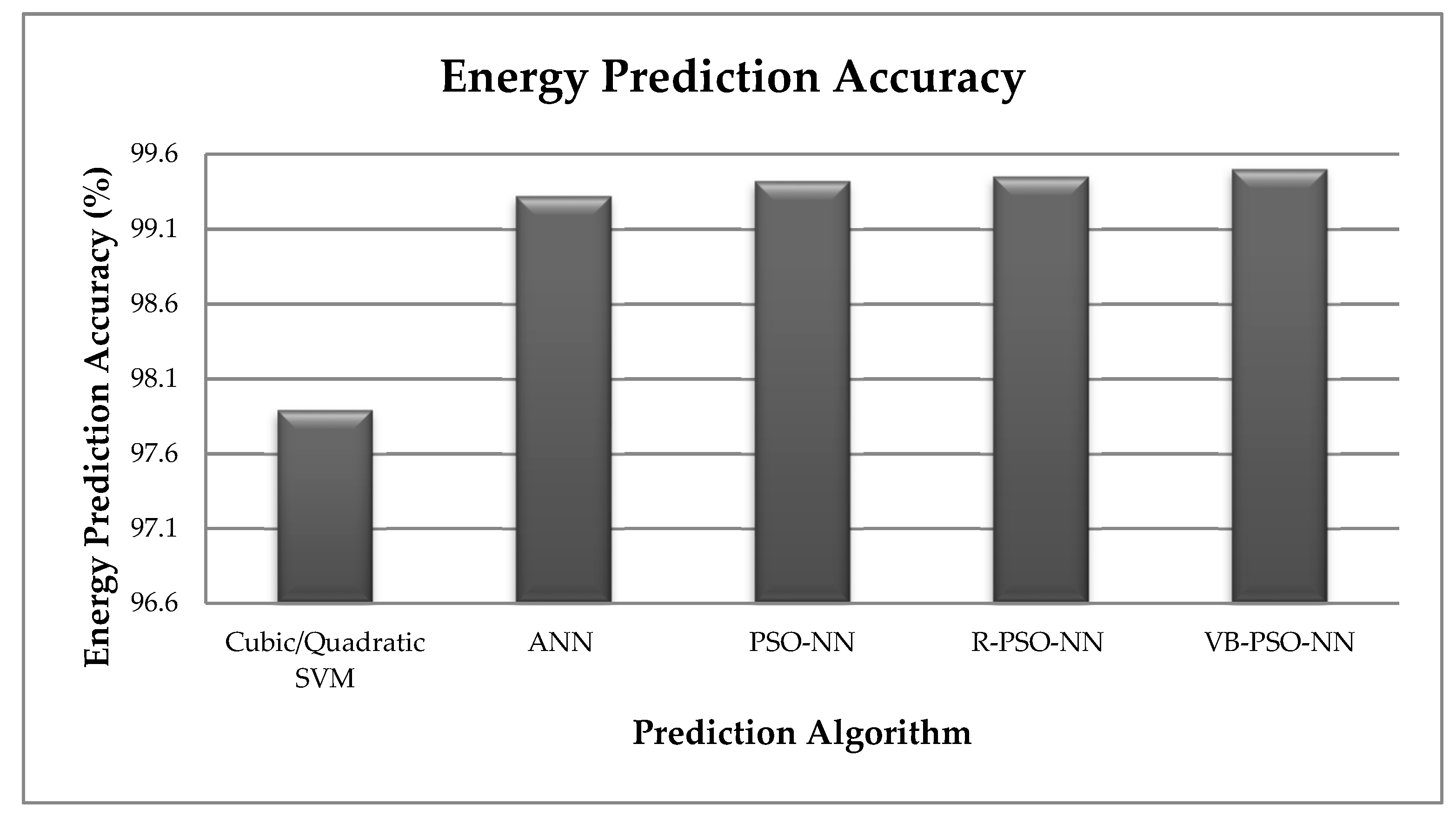
| ANN | 600 | - | 99.32% |
| PSO-NN | 800 | 12 | 99.42% |
| R-PSO-NN | 700 | 12 | 99.45% |
| VB-PSO-NN | 133 | 17 | 99.50% |
© 2018 by the authors. Licensee MDPI, Basel, Switzerland. This article is an open access article distributed under the terms and conditions of the Creative Commons Attribution (CC BY) license (http://creativecommons.org/licenses/by/4.0/).
Share and Cite
Malik, S.; Kim, D. Prediction-Learning Algorithm for Efficient Energy Consumption in Smart Buildings Based on Particle Regeneration and Velocity Boost in Particle Swarm Optimization Neural Networks. Energies 2018, 11, 1289. https://doi.org/10.3390/en11051289
Malik S, Kim D. Prediction-Learning Algorithm for Efficient Energy Consumption in Smart Buildings Based on Particle Regeneration and Velocity Boost in Particle Swarm Optimization Neural Networks. Energies. 2018; 11(5):1289. https://doi.org/10.3390/en11051289
Chicago/Turabian StyleMalik, Sehrish, and DoHyeun Kim. 2018. "Prediction-Learning Algorithm for Efficient Energy Consumption in Smart Buildings Based on Particle Regeneration and Velocity Boost in Particle Swarm Optimization Neural Networks" Energies 11, no. 5: 1289. https://doi.org/10.3390/en11051289
APA StyleMalik, S., & Kim, D. (2018). Prediction-Learning Algorithm for Efficient Energy Consumption in Smart Buildings Based on Particle Regeneration and Velocity Boost in Particle Swarm Optimization Neural Networks. Energies, 11(5), 1289. https://doi.org/10.3390/en11051289