Optimal Distribution Network Reconfiguration through Integration of Cycle-Break and Genetic Algorithms

Abstract

This paper presents novel cycle-break (spanning tree generation) algorithms which can be used to find the optimal distribution network topology. These algorithms (adjacency matrix/top-down/bottom-up cycle break) represent a novel way of obtaining radial network topology by cycle regrouping using adjacency matrix or elementary cycle information. Proposed methods assure connected radial network topology and can be used in combination with genetic algorithms to obtain optimal distribution network structure under minimum active power loss or network loading index framework. The cycle-break algorithms are used in initial population generation, crossover and mutation process to enhance the performance of the genetic algorithms in terms of convergence rate. These modifications make the proposed approach suitable for the use on realistic distribution networks without concern of its complexity. The algorithms are tested on a several standard test networks and the results are compared with the other existing approaches.

1. Introduction

This paper presents new approach for optimal distribution network (DN) reconfiguration using the combination of novel cycle break algorithms (based on adjacency matrix (AM) or elementary cycles (EC):‘bottom-up’ (BU) and ‘top-down’ (TD) approach) and genetic algorithms (GA). The cycle break algorithms which use AM or EC information are then integrated with GA process operators, assuring exchange and survival of best genetic material (parts of distribution network topologies) through evolution process.

Early methods for distribution system reconfiguration used series of heuristic rules determined specifically for the loss reduction, load balancing or voltage profile improvement. In [1], Cinvanlar et al. quantified the possible switching combinations by a set of numerical indices which are then used to rapidly order switching combinations in relation to the potential loss reduction associated with them. In [2], Shirmohammadi and Hong proposed an approach that starts from the meshed grid structure and using optimal load flow pattern logic detects (in each step) the switch that minimally disturbs optimal load flow pattern in order to break the network cycles. They applied this procedure successively, until radial topology is obtained. Baran and Wu [3] used a simplified DistFlow method for fast approximate load flow calculations in order to determine optimal branch exchange in single network cycle.

Tahboub et al. in [4] used GA for minimization of annual energy losses considering the actual annual data for the active and reactive power demand and distributed generation profiles. A fuzzy C-means algorithm was used to classify data into respective clusters and to obtain centroids for the GA optimization. Using this procedure a single optimum is found and fixed through the year. In [5] Mendoza et al. detected fundamental loops from which they extracted individuals for crossover and mutation. Problems appear in the crossover phase where there is a possibility of obtaining non-feasible solutions, so the authors suggested applying filters for identification and rejection/modification of such individuals. Tomoiaga et al. in [6] used GA with initial population generation using heuristic branch exchange algorithm and standard crossover and mutation operators. In crossover they found unfeasible genetic material using information from vector of fundamental loops. Distribution network optimization with sequential encoding and GA was proposed in [7]. Switching operations are based on the two strategies: subtractive (beginning from the meshed network obtained by closing all switches until radial network is obtained) and additive (does the inverse by closing one switch at a time until the radial topology is obtained). Tomoiaga et al. in [8] proposed a multi-objective optimization problem which is solved using GA based on NSGA-II. The GA based on spanning trees of undirected graphs was presented in [9]. Heuristic approaches in combination with GA and hybrid GA for obtaining optimal DN topology, are presented in [10]. In [11], an improved adaptive genetic algorithm (IAGA) was developed for capacitor switching optimization and with branch exchange algorithms it makes joint optimization algorithm for network reconfiguration and capacitor control for loss reduction. Recent research has focused on finding linear or convex relaxations of the AC [12,13] or approximate DistFlow [14,15] power flow equations, adapting them to optimal network reconfiguration and power supply restoration problems. In [16] two-stage optimization which includes network reconfiguration and phase balancing is proposed. The method is used to improve voltage profiles, reduce energy losses, and increase network efficiency in low voltage unbalanced grids. In [17] the authors propose modified particle swarm optimization algorithm to determine the optimal network topology with minimum losses. The authors demonstrate system improvements for different network loading levels when optimal network topology is applied. In [18] the authors simultaneously optimizes the network topology and calculated optimal distributed generation (DG) while minimizing line loss cost, Expected Energy Not Supplied, and switch operation cost. The optimization was performed using the combination of binary particle swarm optimization and harmony search algorithm. Recent interest in the subject of distribution network reconfiguration problem is related to automatization and upgrade of communication infrastructure in distribution network at all levels allowing the implementation of such advance functions. In addition, integration of distributed generation, electric vehicles and energy storage together with the possibility of network islanding, makes the distribution system more dynamic requiring more frequent use of such advance functions.

There have are many approaches that employ GA for optimal DN reconfiguration, but most of them have issues with assuring the DN radial topology, have long computational time or suffer implementation difficulties on real-world distribution networks [4,5,6,8,9,10,11]. By analyzing all these approaches and taking into consideration all the DN constraints, proposed cycle-break algorithms based on AM and EC can be recognized as the algorithms that surpasses these problems and do not violate DN radiality and connectivity constraints. The proposed approach is used to determine optimal distribution network topology with the objective function to minimize network active power losses or network loading index.

From the literature review, it is obvious that GAs are a very popular approach used for solving the DN optimal reconfiguration problem. When using a GA for solving optimization problems, it is very important, like in every other optimization method, to choose a good starting point to achieve faster convergence rate and detection of optimal solution. That is why the most issues are related to ineffective initial population generation, which later causes unfeasible individuals which are subsequently rejected in the evolution process due to violation of different network constraints (radial constraint, voltage and loading constraint etc.). Hence, most of the approaches have poor convergence rate and are not suitable for large real-world distribution networks. The novel cycle-break algorithms based on the network AM or EC information proposed in this paper help to solve some of these issues. Significant improvements, in terms of convergence speed and network applicability, are achieved by integrating cycle break algorithms in GA processes like population generation, crossover and mutation.

This paper has two significant contributions. First, it introduces two novel methods for generation of spanning trees using the network AM or EC information. These methods are general and can be applied to other problems from the graph theory like random spanning tree generation or determination of minimum/maximum spanning tree. The other contribution is related to the integration of proposed cycle-break algorithms in the GA processes (initial population generation, crossover, mutation) in a way which assures good genetic material transfer from one generation to another and fulfillment of radiality/connectivity and other operational constraints in each step. At the end of the paper, combined GA and AM/EC cycle break algorithms are applied on standard network test cases to detect optimal network topology with minimal network losses and the results are compared with the other existing methods.

2. Cycle Break Algorithms Based on Network Adjacency Matrix or Elementary Cycles Information

This part describes a novel cycle-break algorithms for generation of spanning trees. The two sets of cycle-break algorithms, differing only in the context of information they use, are described. The first algorithm requires only the network AM and the second set of algorithms use only the EC information to obtain the radial network structure.

The cycle-break algorithm which uses the AM assures radial topology based on information from initial adjacency matrix which is modified each time the network branch is switched off. On the other hand, the approach which uses the EC information doesn’t use the adjacency matrix but rather information regarding all elementary cycles present in the initial meshed network. This approach uses well-defined rules to reorganize elementary cycles every time when a network branch, belonging to any of the defined elementary cycles, is switched off.

Both set of the algorithms starts with the meshed distribution network (graph) so initial AM and EC cycle information is obtained for this meshed network. Although the distribution network structure is changing through algorithm steps, the AM and EC information obtained for the initial meshed network is always applied as a starting point so there is no need for the additional network traversing after the topology modifications. These topology changes, in relation to the initial meshed network topology, are accounted for through the AM and EC information modifications, using the procedures which are described later on.

2.1. Cycle-Break Algorithm Using Network Adjacency Matrix

The AM cycle break algorithm starts with the meshed network (graph) structure. Algorithm assumes that the network isn’t multigraph, meaning that it doesn’t contain multiple edges/lines (parallel edges or a multi-edge) that are incident to the same two buses (vertices). If the network contains multiple edges, it is trivial task to break these simple cycles. For example, if the objective function is to minimize the network losses, simply switch off all parallel lines between two busses except the line with a minimum line resistance. If the objective function is to minimize the network loading index, simply switch off all parallel lines between the two busses except the line with a maximum rating.

Cycle–break algorithms which use AM or EC information require network bus renumbering for the networks with multiple supply points. This means that in the process of generating radial topology, the algorithm temporarily assigns same bus number to all supply points (and change branch labels for branches connected to network supply points) and generates AM or finds elementary cycles for such bus labeling. In the process of running power flow calculations, the network data is returned to the original bus/branch labelling scheme in order to allow different reference voltages for the network supply points.

The novel cycle-break algorithm which utilizes the network AM is implemented in two stages. The recursive pseudocode for both stages of the algorithm 1 is shown below.

Algorithm 1. Pseudocode for AM cycle break algorithm.

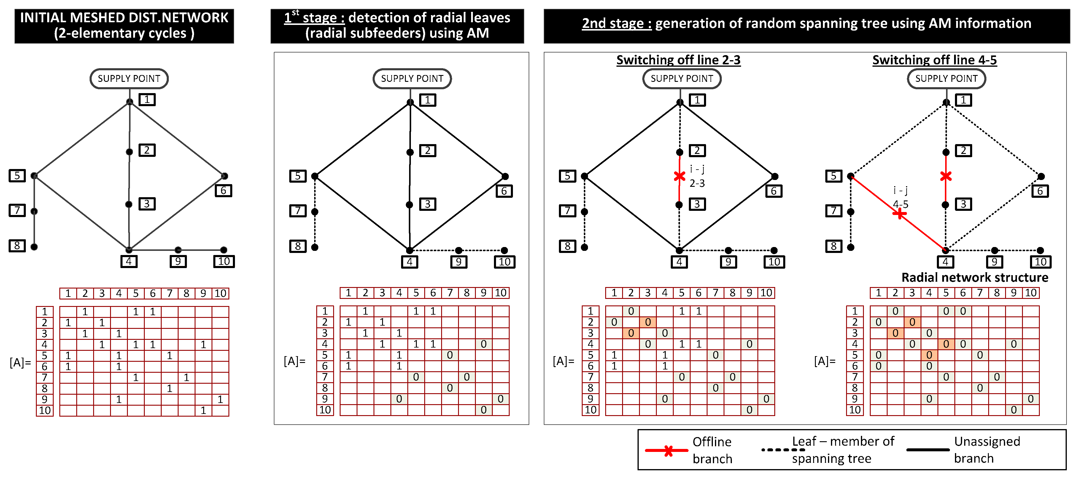
In the first stage, the algorithm finds all network branches (graph leaves) whose exclusion would lead to the isolation of some parts of the network. The lines that are detected in this process have to be part of the network’s radial structure (members of a spanning tree). This search process is based on the recursive detection of network external busses/vertexes (those having connectivity degree of 1), and a removal of line/edge that is incident to that bus/vertex. The network AM is modified every time a new network external bus is detected and adjunct line is removed. After the 1st step of AM cycle break algorithm, modified AM that indicates the remaining lines/edges which constitute network elementary cycles is obtained. For the network shown in Figure 1, the algorithm would first detect bus 8 as the external bus and removed incident line 7–8 from the AM. This would result in bus 7 becoming new external bus and the algorithm removing incident line 5–7 from AM. Given that bus 5 has connectivity degree of 2 after this step, the algorithm would detect bus 10 as the next external bus, and would proceed in a similar manner. By applying the described procedure for the network shown on Figure 1, in 4 iterations the algorithm is able to detect lines 5–7, 7–8, 4–9 and 9–10 as part of the spanning tree/radial network structure. These lines are removed from the network AM in the stage 1 of the algorithm, and after this the algorithm enters stage 2.

In the stage 2, the AM cycle break algorithm enters the process of breaking elementary cycles without the need for even detecting these elementary cycles. In the process of a random spanning tree generation, the arbitrary line is selected for opening (to break single elementary cycle) if the AM element indicating this connection is different from zero. After randomly switching off single line, the AM is modified by removing this connection. After this, the algorithm searches for the network external buses starting from the buses/vertices which are incident to the line that was switched off. This way, the algorithm identifies and prohibits switching-off power lines which would have led to the isolation of some parts of the network. For example, if the algorithm randomly chooses to open line 2–3 it starts a guided recursive search for external buses starting from buses 2 and 3 and detects lines 1–2 and 3–4 as network leaves and members of network radial topology (Figure 1). This procedure is repeated as many times as there are elementary cycles in the meshed distribution network. After all elementary cycles are opened, radial network structure (spanning tree) is obtained together with the zero value for the AM as indicator. The AM cycle break algorithm applied in this way, represents a method to generate random spanning trees for undirected graphs. The algorithm is applied in initial population generation process, crossover process and mutation process of the genetic algorithm.

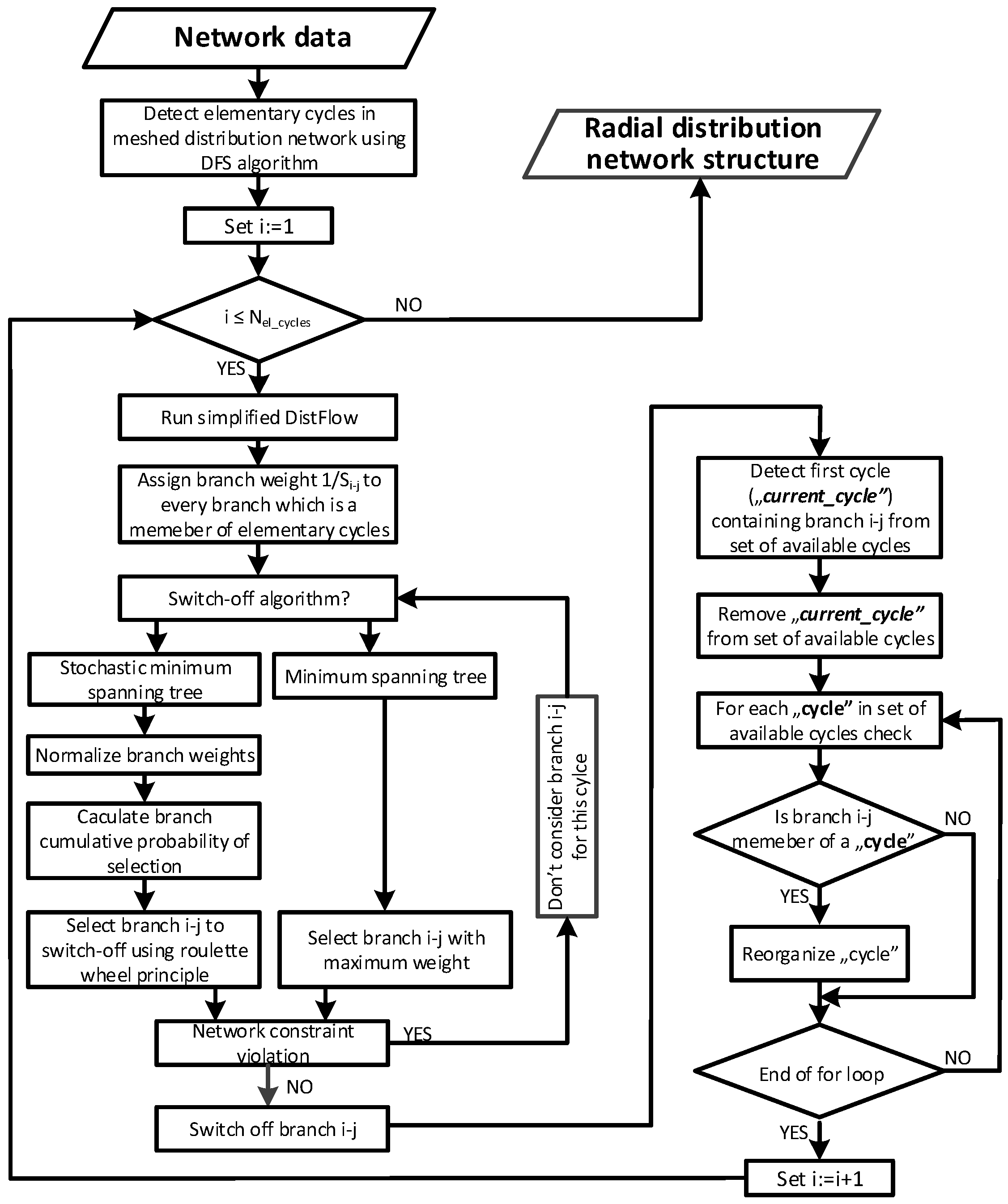
In order to use this algorithm for optimal distribution network reconfiguration, it is necessary to modify the way that branches are switched off. The algorithm is modified in a sense that branches are not selected randomly (as described in step 3: of AM_spanning_tree(A) procedure), but rather heuristically, by assigning the weight to each branch in a specific manner. The weights are calculated by running simplified DistFlow [3] load flow and assigning the weight to each branch in the amount that is a reciprocal value of an apparent power flowing through that branch. These values are updated every time a single branch is switched-off. The basic AM cycle break algorithm is modified to account for the assigned weights and used to generate minimum or stochastic minimum spanning tree with dynamically changing branch weights. In order to account for network constraints, like maximum element loading and bus voltage limits, the switching operation is allowed only if it doesn’t violate these constraints. The basic concept of this algorithm is illustrated by a flowchart in Figure 2.

The generation of initial population, through a minimum spanning tree switch-off algorithm, provides radial distribution network topology with power flow profile similar to the optimal load flow pattern. The optimal load flow pattern equals to the network load flows for the meshed distribution network. This load flow pattern will produce the lowest network active power losses, so a radial distribution network topology with a lowest impact on such load flow patterns is a good starting point for the genetic algorithms with the objective to minimize network losses. Given that the minimum spanning tree switch-off algorithm will always produce same radial network topology, all but one individual in initial population is generated using the stochastic minimum spanning tree switch-off algorithm. This way, a diverse initial population is obtained with different radial network topologies that are likely to be concentrated near the optimal radial network solution.

2.2. Cycle-Break Algorithms Using EC Information

This part presents additional novel algorithms for the spanning tree generation which use information regarding the graph/network elementary cycles. Both TD and BU cycle break algorithm are general and can be applied to other problems from the graph theory like random spanning tree generation or determination of the minimum/maximum spanning tree. The elementary cycles can be detected using the depth-first search (DFS) algorithm [19,20]. The DFS algorithm is called only once for the meshed network and the information regarding EC is later used to generate radial network topologies, regardless of the network topological changes. The important contribution of these algorithms is a fulfilment of the radial network topology constraint, without imposing filters and topology rechecking after the implementation of the algorithms.

The general framework of the algorithm is given by flowchart presented in Figure 3. As shown in Figure 3, TD/BU cycle break algorithm uses minimum (for single individual), or stochastic minimum spanning tree (for multiple diverse individuals), switch off algorithms in the same way as the AM cycle break algorithm. The major difference is related to the cycle break mechanisms. Given this, in the following subsections we present two different cycle break algorithms which use EC information: top-down and bottom-up CB algorithm.

2.2.1. Top-Down Cycle Break Algorithm

In each iteration of the TD cycle break algorithm, one network branch is switched off and a single cycle is broken. This cycle is then removed from the set of elementary cycles. After that, algorithm reconfigures remaining set of cycles if reconfiguration criteria are met. The pseudocode for the random spanning tree generation, using the novel TD cycle break algorithm, is defined with Algorithm 2.

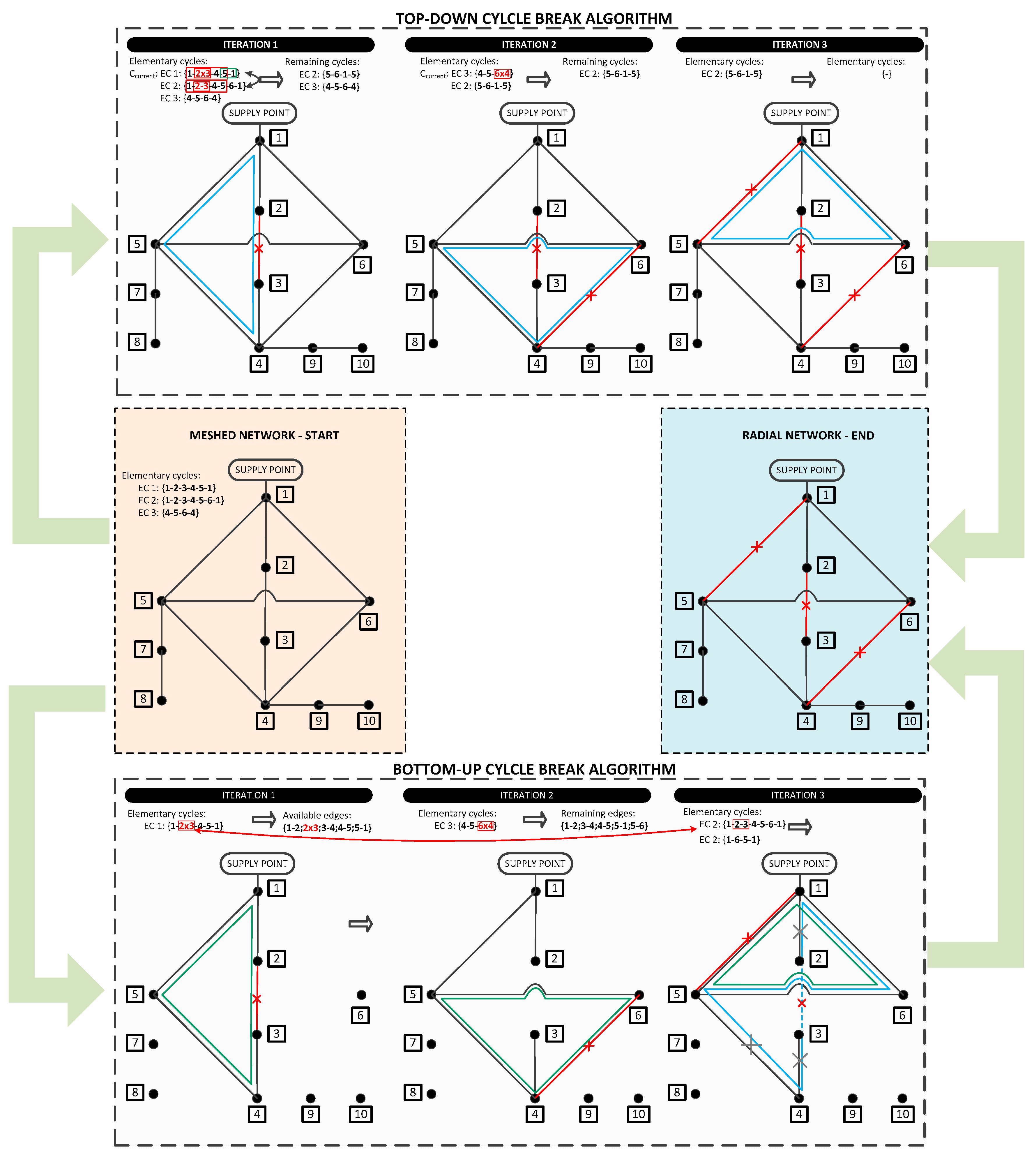
The basic concept of the algorithm is illustrated on the Figure 4. For example, in the first iteration the algorithm chooses to open line 2–3, which is detected as a member of elementary cycle EC_1. This switching action brakes elementary cycle EC_1. However, given that the line 2–3 is also a member of the EC_2, it is necessary to reconfigure the EC_2 to reflect a new network topology. The intersection between the cycles EC_1 and EC_2 consists of a set of lines 1–2, 2–3, 3–4 and 4–5 which are then removed from the EC_1 and EC_2. Remaining lines from the EC_1 (only line 1–5) are then transferred to EC_2, making cycle with lines 5–6, 6–1, 1–5. This procedure is not applied on EC_3, given that this cycle doesn’t contain line 2–3 that was switched-off in iteration 1. Through this cycle reconfiguration process, we have updated elementary cycles to reflect current network topology, without the need for graph/network traversal.

Algorithm 2. Pseudocode for TD cycle break algorithm.

In iteration 2, the algorithm chooses to open line 4–6, which is detected as the member of EC_3. Given that the line 4–6 is not a member of remaining EC_2, this cycle remains unchanged throughout this iteration. In the final iteration 3, the algorithm randomly chooses to open line 1–5, which is member of EC_2, and by doing so breaks the last EC and forms a radial network structure.

2.2.2. Bottom-Up Cycle Break Algorithm

The BU cycle break algorithm uses similar principles of cycle reconfiguration, just like the TD cycle break approach. In every iteration, the algorithm checks if the current elementary cycle contains any of the already opened lines from the previous iterations, in which case it proceeds to the cycle reconfiguration. Pseudocode for BU cycle break algorithm is given with Algorithm 3.

Algorithm 3. Pseudocode for BU cycle break algorithm.

procedure => BU_cycle_break()

1: set nb_cycles:=0; tie_lines=[];

2: for current cycle Ccurrent in EC do

3:  while true do

4:  if any edge in cycle Ccurrent is

member of tie_lines

5:   determine previous cycle Cprev used to

turn off that tie_line

6:   cycle_reconfiguration(Ccurrent, Cprev)

7:  else

8:   false

9:  end if

10:  end while

11:  randomly choose$i,j \in \left[1,\dots ,N_{bus}\right]$such that edge

$E_{i-j}$is member of cycle Ccurrent

12:  set nb_cycles++

13:  set tie_lines[nb_cycles,:]=[i,j];

14: end for

The process of elementary cycle reconfiguration is nicely shown in iteration 3 of the BU cycle break algorithm, which is illustrated on Figure 4. In iteration 3, we are breaking EC_2 of our meshed network. Given that EC_2 contains line 2–3, which was opened in the process of breaking EC_1, we proceed to cycle reconfiguration between EC_2 and EC_1 using the same procedure (cycle_reconfiguration()) as in the TD cycle break algorithm. This changes EC_2, which now contains a set of lines 1–6, 6–5 and 5–1. Given that the current set of lines, which forms a transformed EC_2, doesn’t contain any of previously switched-off lines (2–3, 4–6), we stop with the reconfiguration of EC_2 and randomly choose to open any of the lines from the transformed EC_2.

The pseudocode for the TD and BU cycle break algorithm can be used for random spanning tree generation. In order to use these algorithms in optimal network reconfiguration problems (for initial population generation, crossover and mutation process), we have to select lines to switch-off in heuristic manner, using (stochastic) minimum spanning tree switch off algorithm as shown in Figure 3, considering network load flows and operational constraints. The principle of weight assignment is the same as for the AM cycle break algorithm.

3. Integration in Genetic Algorithm Operations

The optimal network reconfiguration using GA is significantly improved, in terms of convergence speed and solution quality, by integrating the AM or EC cycle break algorithms in all GA operators. In addition to that, other improvements are introduced in the crossover and mutation process of the GA.

The initial population is generated using the AM or EC cycle break algorithms in a way that was described in section II. These algorithms are used to generate population with individuals which are good starting point for GA, thus significantly reducing the computational time to find an optimal solution.

Once the initial population is created, the fitness function for each individual is calculated as shown in the Equations (1) or (2). The proposed approach can be used to find the optimal distribution network topology, either with minimal active power losses (Equation (1)) or minimal network loading index (Equation (2)).

Given that genetic algorithms are usually used to maximize fitness functions, the fitness functions for the two separate objectives are formulated, as described below in order to reduce the problem to the maximization of fitness functions:

$$maximize\to fitness \left(i\right)=\frac{1}{1+P_{loss}\left(i\right)}$$

(1)

$$P_{loss}={\displaystyle \sum }_{k:\left(i,k\right)\in W^B}{r}_{ij}\frac{p_{ji}^2+q_{ji}^2}{v_j^2}$$

$$maximize\to fitness \left(i\right)=\frac{1}{1+P_{load\_idx}\left(i\right)}$$

(2)

$$P_{load\_idx}={\displaystyle \sum }_{k:\left(i,k\right)\in W^B}\frac{\sqrt{P_{ik}^2+Q_{ik}^2}}{S_{ik}^n}$$

Distribution load flow equations are given with following set of equations:

$${\displaystyle \sum }_{k:\left(i,k\right)\in W}^{ }{p}_{ik}=p_{ji}-r_{ij}\frac{p_{ji}^2+q_{ji}^2}{v_j^2}-p_i^L \forall i\in B$$

(3)

$${\displaystyle \sum }_{k:\left(i,k\right)\in W}^{ }{q}_{ik}=q_{ji}-x_{ij}\frac{p_{ji}^2+q_{ji}^2}{v_j^2}-q_i^L \forall i\in B$$

(4)

$$v_i^2=v_j^2-2\left(r_{ij}{p}_{ji}+x_{ij}{q}_{ji}\right)+\left(r_{ij}^2+x_{ij}^2\right)\frac{p_{ji}^2+q_{ji}^2}{v_j^2} \forall i\in B\backslash B^S$$

(5)

subject to network constraints:

$$v_i^{min}\le v_i^{ }\le v_i^{max} \forall i\in B\backslash B^S$$

(6)

$$v_i^{ }=v_i^{ref} \forall i\in B^S$$

(7)

$$\sqrt{p_{ji}^2+q_{ji}^2}\le S_{ij}^n \forall k:\left(i,j\right)\in W^0$$

(8)

where:

$P_{loss}\left(i\right)$ Network active power loss for individual i;

$P_{load\_idx}\left(i\right)$ Network loading index for individual i;

$p_{ij}^{ }$ Real power flow from bus i to j

$q_{ij}^{ }$ Reactive power flow from bus i to j

$p_i^L$ Net (load-production) active power injection at bus i

$q_i^L$ Net reactive power injection at bus i

$v_i^{ }$ Voltage at bus i

$B$ Set of nodes

B^S Set of supply point nodes

W Set of branches

W⁰ Set of online branches

$r_{ij}$ Resistance of branch between nodes i and j

$x_{ij}$ Reactance of branch between nodes i and j

$S_{ij}^n$ Nominal power of the branch between nodes i and j

Equation (3) represents the bus active power balance and the equation is valid for all busses in the network. Net (load-production) active power injection at bus i is calculated by subtracting the active power flow going through the incident power line supplying the bus i with the active power losses along this line and with active power flows along the lines incident to bus i which are used to supply “downstream” incident busses. Equation (4) represents the bus reactive power balance which is calculated in analogy with Equation (3), with a difference of using the reactive power losses and the reactive power flows. Equation (5) is used to calculate the voltage drop along the online network lines, while Equations (6) and (7) define the voltage limits for all network busses. The limits related to the power line capacity of each network branch, are expressed with the Equation (8).

The procedure described in the following sections can be adapted also to other objective functions such as minimization of voltage profile deviations or system reliability index (ENS, SAIDI, SAIFI) improvement. This requires only minor modifications regarding the fitness function formulation and weight assignment process during the initialization and crossover process of the genetic algorithm, but the main concepts related to the application of the cycle break algorithms and methods of performing operations inside the genetic algorithm remain the same.

The fitness function values are used to associate the probability of selection with each individual (radial DN topology) present in the population. Pairs of individuals (parents) which will undergo the crossover process are selected using the fitness proportionate selection also known as the roulette wheel selection. At the beginning of every iteration, specified number of best individuals (elite individuals) is transferred directly to the next evolution epoch unchanged, which assures monotonic increasing improvement of the fitness function throughout the evolution epochs.

In order to integrate the AM or EC cycle break algorithms in the crossover and mutation process, it is necessary to adapt the branch weight assignment. This is described in more details in the next subsections.

3.1. Integrating Cycle Break Algorithms in Crossover Process

In order to enhance the efficiency of the crossover process, two main goals need to be achieved: first it is necessary to assure that the generated offspring has radial network structure without the need for topology rechecking or correction, and second, good genetic material needs to be transferred to offspring to enhance the convergence rate. The transfer of good genetic material from parents to offspring, in reality, means that if same network lines are online in both parents then they should be online in offspring, and if same network lines are offline in both parents then they should be offline in offspring as well.

This transfer of good genetic material from parents to offspring can be achieved by adapting crossover process to specifics of the DN reconfiguration problem. In order to create a single offspring, the algorithm finds intersection and union between a pair of DN network topologies (parents’ pair). This information is used later to assign weights to the distribution network lines that are present in the union of parent topologies.

By creating a network topology, which is determined as a union of parent topologies, the algorithm forms a meshed network structure that represents the “backbone” for the radial distribution network topology, which is determined at the end of crossover process (single offspring). After creating such a network topology, the algorithm assigns zero weights to all the lines that are present in the parent intersection topology. All the other lines, which are present in parent union topology, have weights assigned in a manner described on Figure 2 or Figure 3. In addition to that, all the lines that are offline in both parents are also offline in the offspring.

For the network shown in Figure 5, given that both “parent 1” and “parent 2” topologies have lines 1–2, 3–4, 1–6, 5–7, 7–8, 4–9 and 9–10 online, these lines are assigned with a zero weight. In both parents, line 4–6 is switched off, so it is also switched off in the offspring. All the other lines in a union of parents (1–5, 2–3, 4–5, 5–6) have weights assigned according to the procedure described in Figure 2 or Figure 3. By using (stochastic) minimum spanning tree switch-off algorithm, it is possible to create offspring from this weighted network subgraph. This is achieved by integrating the AM or EC cycle break algorithm in the crossover process.

The process of integrating the AM cycle break algorithm in the crossover process is trivial. We generate AM for the topology that is a union of parents and apply the procedure described with a flowchart shown in Figure 2. The only difference is that line weights need to be fixed to zero value for all the lines that are member of a parent intersection topology in all iterations.

The process of integrating EC cycle break algorithm in the crossover process can be performed in two ways. The slower and easier way that requires network traversal, consists of detecting new EC by applying DFS algorithm [19,20] on network topology which is formed as a union of the parent topologies. The remaining part of the process is described with a flowchart shown in Figure 3, with the same difference, as for the AM cycle break algorithm, related to fixing zero weight to some of the network lines.

The faster way, which doesn’t require network traversal, uses EC information obtained for the initial meshed distribution network. After detecting which lines are switched off in both parents, the algorithm reorganizes elementary cycles obtained for meshed network topology to reflect new state of distribution network. Reorganization of EC is performed using the same principle as described in Section 2.2. The difference is that not random but specific lines need to be turned off to reconfigure EC for current state of DN. For example, for network shown in Figure 5, we see that line 4–6 is offline in a union of parent topology. To modify EC information the algorithm detects line 4–6 as member of EC3 {4-5-6-4} (Figure 4). This means that this cycle doesn’t exist in topology shown on Figure 5, which was obtained as a union of parents. Also, given that line 4–6 is not a member of EC1 {1-2-3-4-5-1} and EC2 {1-2-3-4-5-6-1}, it is not necessary to reconfigure these two ECs. If, for example, line 4–5 would be offline, then both EC1 and EC2 would have to be reconfigured, given that line 4–5 is a member of these cycles. Cycle reconfiguration, when needed, can be performed using procedure described for the TD cycle break algorithm. By using this approach, we can eliminate the cycles which don’t exist in a union of parent topologies and reconfigure the cycles which remain in this network topology. All this is performed without the need for additional network traversal, using only EC information obtained once for initial meshed network topology.

3.2. Integrating Cycle Break Algorithms in Mutation Process

Mutation process with the AM or EC cycle break algorithm is slightly different, compared to the crossover. Each offspring obtained throughout crossover process undergoes mutation if the generated random number has value lower than a specified mutation probability. The mutation process assumes random closure of one offline branch in a network which forms a single cycle in the network. Using AM or EC cycle break algorithm, this cycle is then broken producing a different radial DN network topology. This makes mutation process fast and simple.

After the mutation process, the specified number of individuals with the lowest fitness function values is substituted with the same number of parents which have the highest fitness function. Introduction of elite individuals accelerates convergence rate by preventing the best individuals from each evolution epoch to be lost or substituted by the inferior individuals.

4. Case Study

Algorithms described in previous sections are implemented in MATLAB (MathWorks, Natick, MA, USA). Tests were performed on a Windows machine equipped with an AMD six-core (3.3 GHz) processor and 8 GB of RAM. Tests are conducted on standard network test cases for 70, 136 and 880 bus systems to prove applicability for both small and large DN networks. The basic network data for these networks is summarized in

Table 1. Basic network data for 70, 136 and 880 bus network.

Buses (Nbus)	Supply Points (NSP)	Lines (Nbr )	Sectionalizing Switches	Tie Switches	Initial Losses (kW)
70	2	76	68	8	33,745
136	1	156	135	21	32,040
880	7	900	873	27	149,630

while the full network models are described in [21,22,23]. These networks were also considered by Taylor and Hover in [14] which allows us to compare the proposed approaches with the results obtained using mixed integer quadratic programming (MIQP), mixed integer quadratic constrained programming (MIQCP) and mixed integer second order cone programming (MISOCP) approximations described in [14]. In order to achieve this, and provide adequate numerical comparisons, we implemented approaches based on MIQP, MIQCP, and MISOCP in General Algebraic Modeling System (GAMS) [24] and solved underlying problems using CPLEX software (IBM, Armonk, NY, USA) [25].

The proposed algorithm was tested with GA parameters as follows: maximum number of iterations = 20; population size = 20; mutation probability = 0.2; number of elite individuals = 1. The cycle break algorithm that is used in the initialization phase, crossover and the mutation phase of GA is based on the TD cycle break algorithm. The execution times for other cycle break algorithms are approximately the same, due to the same level of complexity for the AM, TD and BU cycle break algorithms we proposed.

4.1. Results

The optimal network topologies, as well as loss reduction in relation to initial topologies, are given in

Table 2. Initial and optimal network topology for 70, 136 and 880 bus network.

Test Network	Initial Network Topology		Optimal Network Topology		Power Loss Reduction (%)
	Offline Branches	Losses (kW)	Offline Branches	Losses (kW)
Network I (70 bus)	69;70;71;72;73;74;75;76	33,745	30;39;45;51;66;70;71;76	29,860	11.51%
Network II (136 bus)	136;137;138;139;140;141;142; 143;144;145;146;147;148;149; 150;151;152;153;154;155;156	32,040	7;35;51;90;96;106;118;126; 135;137;138;141;142;144; 145;146;147;148;150;151;155	27,992	12.63%
Network III (880 bus)	874;875;876;877;878;879;880; 881;882;883;884;885;886;887; 888;889;890;891;892;893;894; 895;896;897;898;899;900	149,630	84;130;141;159;190;282;288; 306;312;409;411;452;494;596;616; 630;631;637;698;815;844;885;888; 889;890;896;900	45,700	69.46%

. The level of loss reduction differ between test networks depending on the initial network topologies ranging from relatively low 11.51% for 70 bus test network to extremely high reduction in the amount of 69.46% for 880 bus network. For all the test networks, the proposed approach identified reported global optimum solutions, regardless of the network size.

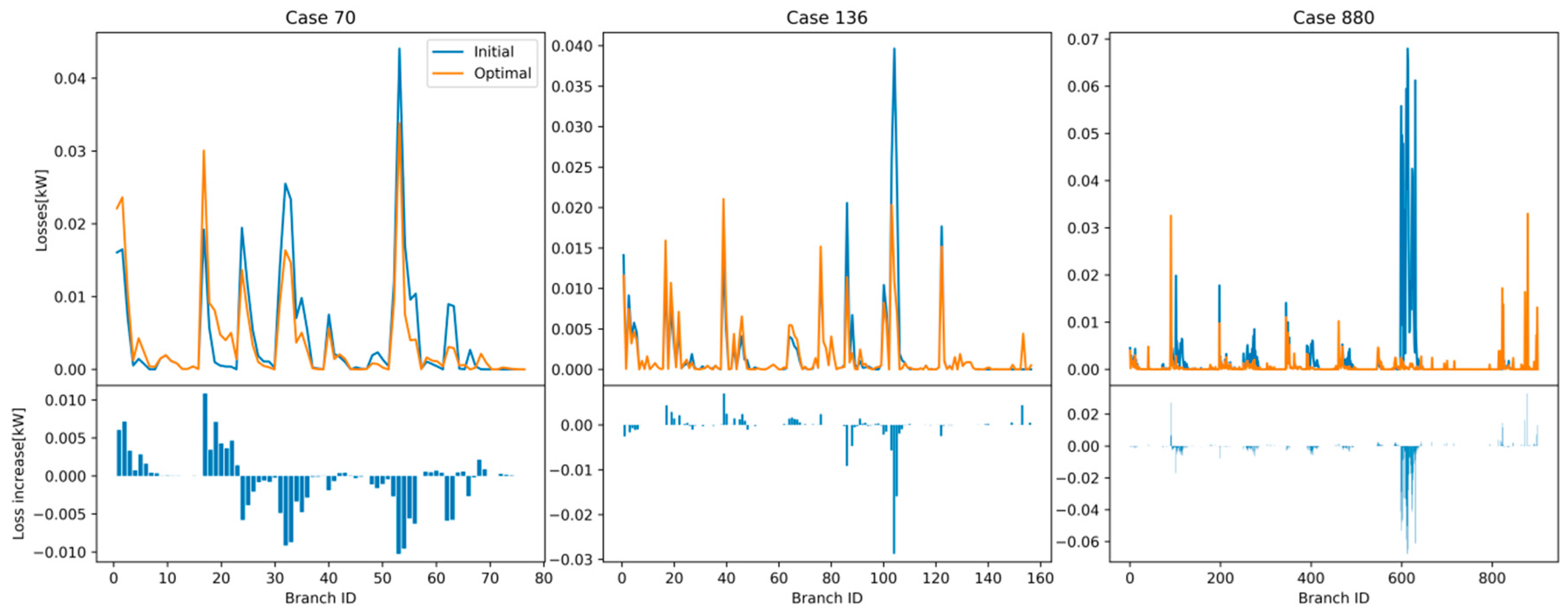
Figure 6 presents branch losses for 70, 136 and 880 bus network, for the initial and the optimal topology, together with the power loss difference for each network branch. We can see that, although there is an increase of power losses along certain branches, by applying optimal network topology, decrease of the losses on other branches is more pronounced, leading to the loss reduction at a network level.

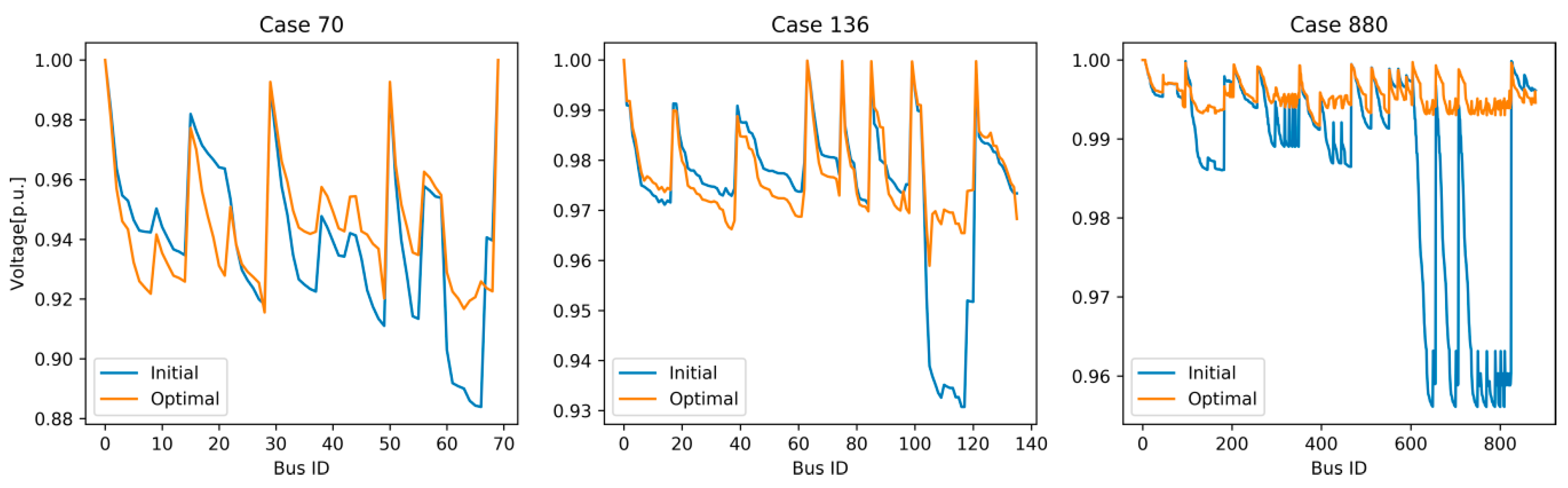
Although the objective of distribution network topology optimization was to reduce network losses, by applying optimal network topology, significant improvement of network voltage profile is achieved as well (Figure 7). This is most evident for a 70 bus network, which has low voltages for the initial network topology, with voltages reaching as low as 0.884 p.u. (11.6% voltage drop).

Such low voltages represent power quality issue, given that they are far below the limits defined by the power quality standards. By applying optimal network topology, the voltage profile was improved considerably and brought to the normal limits.

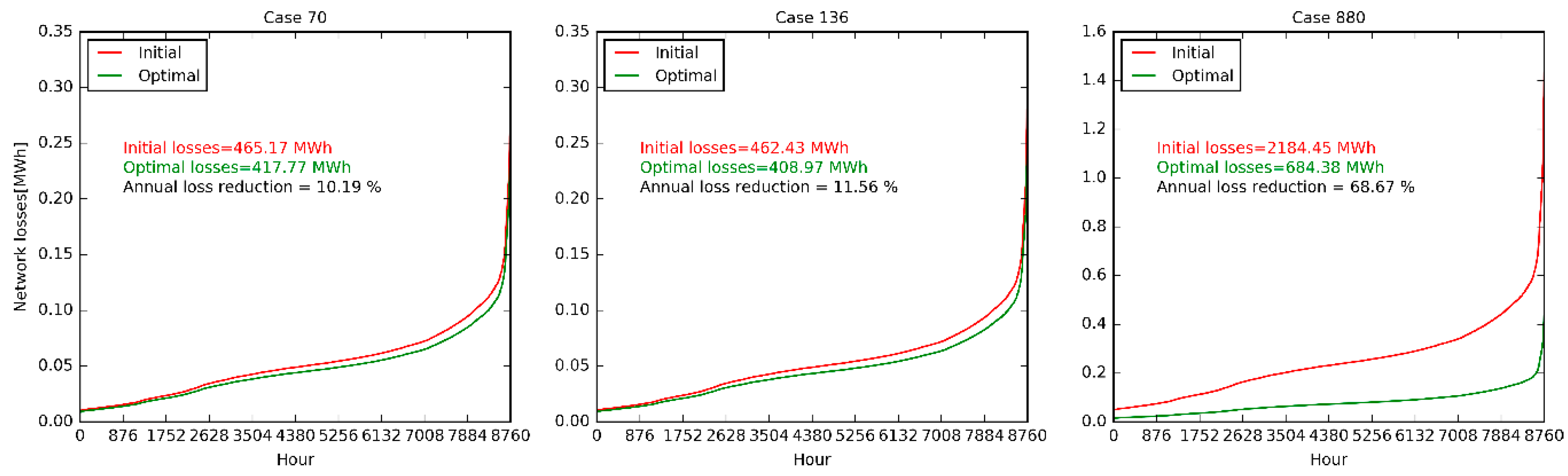
Based on the measured average hourly data of network load for period of one year (data from real distribution network), annual energy losses were calculated for initial and optimal network topology for the considered networks. Figure 8 shows relative chronological load (in relation to peak demand), as well as load duration curve which was considered in this analysis.

Based on the hourly load data, energy losses were calculated for the initial and the optimal network topology. Figure 9 shows loss duration curve for the considered networks as well as annual energy losses for the initial and the optimal network topology. Reduction of annual energy losses ranges from 10.19% for 70 bus network to 68.67% for 880 bus network which is approximately similar to the reduction of power losses calculated for the peak load (Table 2).

4.2. Computational Time

Table 3. Comparison of computational time for different approaches.

Test network	Proposed Approach		MIQP [14]		MICQP [14]		MISOCP [14]
	Obj.value (MW)	Time (s)	Obj.value rel.gap (%)	Time (s)	Obj.value rel.gap (%)	Time (s)	Obj.value rel.gap (%)	Time (s)
Network I (70 bus)	0.2986	3.54	0.3009 0.0093	0.562	0.3002 0.0191	2.688	0.2993 0.0199	36.308
Network II (136 bus)	0.2799	23.20	0.2815 0.0137	7.745	0.2901 0.0159	4.999	0.2833 0.0357	T.L. >36,000
Network III (880 bus)	0.4570	47.99	0.4586 0.0200	11,038	0.4765 0.0199	18,312	0.5039 0.1964	T.L. >36,000

summarizes the computational time for different approaches. The MIQP, MICQP and MISOCP approximation of Taylor and Hover [14] was implemented with a relative gap of 2% and maximum computational time limit set to 10 h. The final objective values for these approaches were obtained by running full AC power flow [26] after obtaining the integer solution based on approximate DistFlow.

We can see from the results shown in Table 2 that these approaches require smaller relative gap in order to find reported global optimal solution, which would significantly extend computational time for these approaches. Also, from the computational time, we can see that these approaches suffer from the computational inefficiencies and are therefore not adequate for larger and more complex distribution networks. Moreover, the MIQP and MICQP approach presented in [14] doesn’t consider bus voltage limits.

On the other hand, proposed approach which integrates cycle-break and genetic algorithms, is able to detect global optimum solutions for all the test networks. For smaller networks, the algorithm produces network topologies with lower objective values (lower network losses), but with higher computational times. In this analysis, we assume that the method converged if we obtain global optimum solution in three consecutive evaluation epochs. The proposed method shows better performance in relation to MIQP, MICQP and MISOCP approach, in the sense of objective function value and execution time for larger distribution networks, producing optimal solution in a fraction of the time of these approaches.

Results shown in Table 2 and Table 3 are obtained with a cycle break algorithm that uses minimum spanning tree switch off strategy. Figure 10 shows convergence characteristics of the proposed approach for different cycle break switch off strategies (stochastic vs. minimum spanning tree). We can see that the proposed cycle break algorithms, employing minimum spanning tree switch-off strategy, provide batter population initialization and faster convergence rate in relation to the stochastic minimum spanning tree approach. Despite of this, both switch-off approaches are able to identify the optimal network topology in time frames shorter than MIQP, MICQP and MISOCP approaches, for large distribution networks.

5. Conclusions

This paper presents novel cycle break algorithms which use network AM or EC information to produce radial network structures. The AM cycle break algorithm uses adjacency matrix information for the meshed grid, which is modified with each branch elimination through a recursive guided matrix search. On the other hand, EC cycle break algorithms (TD and BU approach) use information regarding elementary cycles for meshed network, which are then reorganized with each branch elimination to reflect a current network state.

The developed algorithms are integrated with a genetic algorithm to solve the optimal distribution network reconfiguration problem, with a focus on the network loss reduction or network load balancing. Specific approaches described in this paper assure always feasible network solution, without the need for constant rechecking of network radiality and connectivity constraints and optional topology modifications when these constraints are violated. Enhancements like this significantly accelerate convergence rate and reduce computation time, which was demonstrated on a small scale and a large scale distribution networks considered in the paper. The reduction of network power losses was achieved in the range of 11.5 to 69.5%, depending on the network initial topology and network parameters. In addition to this, significant voltage profile improvements were achieved through the network topology optimization. The main contributions of this paper can be further summarized as follows:

• Development of novel cycle-break (spanning tree/forest generation) algorithms, based on elementary cycle information or adjacency matrix information. These algorithms show high computational efficiency in relation to other similar greedy algorithms when repetitive calculations are needed. Proposed cycle-break algorithms can be applied to large spectrum of problems, other than the one presented here.
• Integration of cycle-break algorithms in genetic algorithm process to assure solution feasibility in a sense of radiality constraints, which was often the problem in similar approaches.
• Development of method which integrates cycle-break algorithms and genetic algorithms to solve optimal distribution reconfiguration problem in computationally efficient way, making the method applicable to realistic distribution grids.