Abstract
The amount and distribution of land which is eligible for renewable energy sources (RES) is fundamental to the role these technologies will play in future energy systems. Unfortunately, land eligibility (LE) investigations in the literature are plagued by many inconsistencies between studies, impeding the work of researchers and policy makers interested in energy system development planning. As one factor contributing to this, the criteria used to construct land exclusion constraints have not been the focus of scientific investigation on a large scale, and as such their interactions are not well known.Therefore, an open source LE framework was used to perform evaluations in the European context of 36 commonly used constraints. After direct visualization, three measures by which these constraints are valuable to an LE analysis were computed: independence, exclusivity, and overlap. Results show extensive spatial sensitivity to constrain influence. Furthermore, some constraints, such as proximity to agriculture and woodland areas, rank high in all three measures; others, such as distance from airports and camping sites, consistently rank low; and still others, such as elevation, score highly in one measure but not the others. With these results, LE researchers can better understand the contributions of the constraints used in their analyses.
1. Introduction
As many world economies aim to meet emission reduction targets, countries will need to carefully consider the options available to them when choosing how to develop their energy systems. Choosing a particular developmental pathway is a challenging endeavor, however, given the uncertainties of future climate impacts and evolving sociotechnical landscapes. Therefore, an effort must be made to explore as much as possible the different pathway options available and future scenarios that might arise. In this regard, progress is being made in the form of energy system design models and similar analyses which serve to evaluate these pathways [1,2,3].
Judging from recent trends, renewable energy sources (RES) will certainly play a significant role in the energy mix of the evaluated developmental pathways [4,5]. Amongst other technologies, this will likely include land-intensive RES technologies, such as on- and off-shore wind turbines, photovoltaic (PV) arrays, concentrated solar power (CSP) parks and biomass processing plants. Well known issues that these technologies entail, such as intermittent [6,7] and spatially-dependent [8] power production, have been the focus of intense research for many decades. Nevertheless, many uncertainties and unanswered questions prevent the guarantee of successfully implementing large-scale RES technologies into future energy systems. Of these uncertainties, the influence of sociotechnical criteria, such as nature conservation, disruptions to local citizens, and unfit terrain on the distribution of RES technologies across a region, is outstanding. When small or otherwise uniform study regions exhibit little variance in their spatial characteristics, the consequences of a variable distribution can be largely ignored or simplified, yet, as evaluations progress towards larger spatial scope, this variability quickly becomes a crucial quality to consider [9]. One of the main reasons this issue remains outstanding, however, is that the response of a region to these sociotechnical criteria is not only dependent on the technology being considered, but can also vary significantly between regions [10] and can even change over time [11]. Nevertheless, incorporating the influences of these sociotechnical criteria is fundamental to properly treating RES distribution, and by extension production, when evaluating energy system developmental pathways.
The application of sociotechnical criteria to RES distribution has, in fact, received significant attention from the research community [12,13,14]. One simple avenue in which the literature uses these criteria to influence RES distribution is the concept of land eligibility (LE); the application of one or more exclusion constraints (constraints are simply a restricted usage of criteria, and so this term is used from hereon to avoid mixing terminology) to a region to determine the land that is eligible for RES installation. LE was described by Iqbal [2] as one of the typical inputs in the generic energy resource allocation problem, which includes energy system design and many other LE-dependent problems as well. Examples of LE analyses in the literature are common [15,16,17,18,19,20]. Although they operate in differing geographical scopes, in each of these examples, LE has been used to determine the locations available for either onshore wind turbines or open-field PV parks. By doing this, the maximal capacity for these technologies is found in each researcher’s areas of interest, which can influence decisions made by investors and policy makers. Robinius [17] and Samsatli [18] used the results of their LE analysis as an input to an RES capacity optimization scheme in Germany and the United Kingdom, respectively, exemplifying how an LE result can be directly linked to the final design of an energy system.
However, despite its attention from the community, little to no focus has been spent on the criteria themselves. As a result, there appears to be a lack of knowledge of the abstract geospatial qualities of these constraints, and moreover regarding how the application of one or more can impact the result of an LE or similar analysis. The current work aims to address this issue by employing the open source LE model Geospatial Land Availability for Energy Systems (GLAES) [21] to evaluate interactions between 36 constraints defined across the European continent. The evaluated constraints represent those most commonly used to determine the LE of typical RES technologies; including, for example, distance from settlements, roads, protected areas, and power lines. Europe is chosen as the study region due to its dense geopolitical landscape and overall data availability. This report begins with a hypothetical discussion of why an investigation into constraint interaction is compelling, including an overview of the specific aims of this analysis. Following this, a brief description of the model and employed data is provided, after which the analysis methodology is detailed. Finally, results from the analysis are presented and discussed.
2. Constraint Interaction
LE analyses are, and will remain, a crucial piece of energy related research. However, despite being of high interest to the research community, the cumulative sum of knowledge regarding LE is ill-posed to meet the demands of spatially-broad contexts in future analyses. Inconsistency between studies presents itself as the major cause of this situation. Resch [14] previously discussed in detail how inconsistent methodological practices impact the general usage of Geographic Information Systems (GIS) in RES related studies, which includes LE studies. Some main issues discussed are associated with data availability, proprietary formats, singular integration methods, and an overall lack of standardization. Most notably, Resch pointed out that investigators generally perform their own data acquisition and mapping of the relevant information. One issue not discussed, however, is that the widespread inconsistent treatment and lack of abstract knowledge surrounding the constraints which make up LE studies diminishes the comparability between these studies and thereby limits the construction of a broad understanding of this issue. It is clear that an improvement in these areas would be a benefit to the global energy-minded community.
The impact of inconsistent constraint treatment in the literature is exemplified by two LE analyses. In their studies, Samsatli [18] and Waston [22] investigated the LE for onshore wind turbines in southern England. Watson found that 37.8% this area is available while Samsatli found approximately 2%. Clearly, these two studies are not in agreement, but, as Table 1 summarizes, the constraints enforced in either study are quite different from each other and so it is not a surprise that their results differ. For instance, Samsatli imposed strict restrictions around roads and power lines; which will certainly remove a large portion of land. Watson, however, excluded a more broad selection of protected areas (excluding both ‘historically important areas’ as well as ‘wildlife designations’) than Samsatli as well as adding a 1 km buffer around these features. Watson also excluded agricultural areas, which make up a significant portion of Southern England’s landscape [23]. Exclusion of areas beyond 500 m of settlement areas is one common feature of these studies, although a closer inspection reveals that the definitions of what constitutes a residential area are distinct from one another. When considering settlement areas, Samsatli measured the 500 m buffer from ‘developed land’ while Watson excluded 500 m from ‘all dwellings and single properties’.

Table 1.
Constraints imposed by Samsatli [18] and Watson [22] when investigating onshore wind availability in southern England.
The differences between the Samsatli and Watson studies do not invalidate either study, but they do bring up several questions regarding the nature of the constraints that were used. For example, which of these constraints is most responsible for the discrepancy between the reported LE results? In addition, how much of this discrepancy is a result of the different settlement area definitions? Finally, if these constraints were imposed in another regional context, by how much would the discrepancy change? Unfortunately, these specific questions cannot be addressed as the exact data sources for some of the imposed constraints as well as the precise LE methodologies used are not known to the authors of this work. Nevertheless, it is easy to see how these questions can be applied to other LE analyses, and how developing deeper understanding of this area can benefit the community.
Several measures can be used to illuminate the interactions amongst exclusion constraints. When evaluating LE with multiple constraints, it logically follows that some areas are redundantly excluded by more than one constraint, such as areas in Samsatli’s study that are both beyond 500 m from roads and beyond 1500 m from power lines. Since multi-constraint exclusion of a location is no different than single-constraint exclusion, it can then be concluded that certain constraints should be relatively more valuable than others. Of course, a constraint which independently excludes a large proportion of the land is a valuable consideration. This measure of constraint value will be referred to as the independence. In comparison, a constraint which excludes a small area could also be considered as valuable if the excluded areas are exclusive to that constraint. This will be called the exclusivity. In this same way, a constraint which has a high tendency of overlapping the excluded areas of other constraints could also be considered important. This is because the need for possessing detailed data for the overlapped constraints is reduced, as having such data would not significantly change the LE result. This final measure will be referred to as the overlap.
As the specific aim of this paper, an evaluation of 36 common constraints in the European context is performed. First, the constraints are grouped together to decrease complexity, and are directly visualized to determine where they tend to exert their influence. Following this, the relative value of each constraint is found according to the three proposed measures.
3. Methodology
To perform this analysis, the open source LE model GLAES [21] is utilized, along with a set of datasets called Priors which were constructed along with the release of GLAES [24]. Discussion of these tools is broken into three parts. First, the logic behind choosing the 36 constraints evaluated in this analysis is shown. Following this, an overview of the GLAES model and associated Prior datasets is provided. Finally, the method to determine the constraint evaluation measures is detailed.
3.1. Criteria Identification
Identification of the most common constraints to consider is accomplished via a review of the available LE literature. In total, 43 [15,16,19,20,22,25,26,27,28,29,30,31,32,33,34,35,36,37,38,39,40,41,42,43,44,45,46,47,48,49,50,51,52,53,54,55,56,57,58,59,60,61,62] publications representing 53 independent LE analyses were considered, and the constraints included in each case were tabulated. These studies cover many different technologies, although most investigate either onshore wind or CSP plants (although PV and biomass are also present). To find a consensus between the sources, generalizations had to be made regarding the constraint used by the authors taking into account their expressed intentions. Furthermore, constraints which were only used by a single author were removed from this stage of the investigation. A full description of how this procedure was carried out, including a deeper explanation of each of the identified constraints, can be found in the methodological report associated with this work [24].
Table 2 displays the result of this literature review. In the first column the name of each identified constraint is given. Many studies used a general description of some constraints while others made distinctions within these groups, therefore these sub-constraints are listed as well. Additionally, the constraints are divided into four distinct motivational groups to differentiate between the underlying reasons for why the authors included these constraints in their analysis. The Social and Political group refers to constraints which were included due to social preferences or political mandates of local citizens and other stakeholders. The Physical group refers to constraints derived from limitations imposed by physical characteristics of the land, such as the soil type, or presence of a forest. The Conservation group corresponds to constraints related to conservation efforts by local, national, and international organizations. Finally, the Technical Economic group refers to constraints which are fundamentally included for economic reasons, such as excluding distances too far from power lines beyond which connection costs become exorbitant. The term technical is used in this case to indicate that constraints in this group are generally not a result of detailed economic evaluations, but are instead assumed thresholds. Next to this column, the frequency that each constraint was used in the study’s analysis (but not necessarily in the LE analysis) in comparison to all of the reviewed studies is shown. In the following two columns, the typical expression of each constraint is provided in regards to the threshold value chosen by the authors who used these constraints; for example, most studies which considered settlements excluded distances less than 800 m from any settlement. In actuality, the authors used a wide array of values for each constraint which, in some cases, would fluctuate greatly. Along side these typical value columns, the associated methodological report for the GLAES model [24] also provides low and high constraint expressions to show this spread. Two exceptions to this are aspect and irradiance, which have been altered from their typical literature expression. An agreement within the literature regarding how aspect should be measured was not apparent, therefore the measure of degrees in the northward direction was chosen with a typical threshold of 3° N. As for irradiance, the LE studies which include this constraint generally suggested a threshold value around 5 kWh/m day; however, as this is a far too strict value for a European context, a value of 3 kWh/m day is used instead. Finally, although one of the Prior datasets is used to represent each constraint, the fundamental data source which was used is given in the last column. Further background to the Prior datasets is provided in the following section.
Table 2.
Typical constraint expressions for land eligibility (LE) analyses. Constraint values are found as a result of reviewing 53 LE analyses in the literature. The ’Data Source’ column provides the fundamental data source used to represent each of the identified constraints across the European context. These sources include the Corine Land Cover (CLC) [23], the Digital Elevation Model over Europe (EU-DEM) [63], and the World Database on Protected Areas (WDPA) [64].
Due to the European scope of this analysis, a suitable data source could not be found for all of the identified constraints. Therefore, these constraints are not displayed in Table 2. This includes distance to radio towers, gas lines, power plants, earth quake zones, land slide zones, flood plains, specific types of natural vegetation and private land. Furthermore, distance from historically significant sites is also not listed despite its prevalence in the sources seeing as how a consensus could not be found in the literature regarding what constitutes historical significance. Fortunately, all of these constraints appeared in less than 10% of all of the reviewed studies with the exception of historical significant sites (25%) and private land (13%).
3.2. GLAES and Prior Overview
The GLAES model [21] is an open source project developed for the purpose of standardizing the implementation of LE analyses. This project was initialized in part to address the methodological inconsistencies currently present in the LE literature. GLAES is designed to be adaptable to common geospatial data formats, to be scalable to large geographical areas, to minimize expected errors resulting from geospatial operations, and to be methodologically transparent [24]. The model has been implemented in the Python 3 programming language, with primary dependencies on the Geospatial Data Abstraction Library (GDAL) [72] for geospatial operations and on the SciPy [73] ecosystem for general numerical and matrix computations, both of which are also open source projects.
To conduct an LE analysis with GLAES, the following steps must be taken. First, a study region must be defined in the form of a vector file and used to initialize a GLAES analysis. Values for resolution and spatial reference system can also be provided. Following this, multiple exclusion constraints can be applied one at a time by providing GLAES with a data source to exclude from and instructions on how to indicate the areas which should be excluded. The manner by which GLAES accomplishes this depends on the data source. If given a raster source, GLAES will expect a minimal and maximal value defining the pixels which should be excluded. If given a vector source, GLAES can accept a Structured Query Language (SQL)filter string to identify the specific features which should be excluded. Furthermore, these data sources do not need to be expressed in the same projection system as the one with which the analysis was initialized, as GLAES is capable of translating between projection systems as needed. Finally, regardless of the type of source which was provided, GLAES can also be given a buffer value by which the indicated exclusion areas can be grown. Once all of the desired exclusions constraints have been applied, GLAES can generate a raster file of the resulting available areas. For the purposes of this work, all computations in GLAES were performed in the EPSG3035 projection system with a spatial resolution of 100 m.
Along with the development of GLAES, an effort was also made to produce a set of general datasets to represent common geospatial criteria and the outcome of this effort is the so-called Prior datasets. Geospatial criteria are useful for many application besides simply as exclusion constraints in LE analyses, such as in multi criterion decision management analyses. Unfortunately, one of the inconsistency issues in GIS-related modeling heavily discussed by Resch [14] is the inconsistent use of data sources. To address this issue in the European scope, the Prior datasets were created and, like the GLAES model, are also openly available [21].
Each Prior dataset represents a single criterion and is simply a processed version of other open datasets. Furthermore, they are all expressed as byte-valued rasters defined over the European context. As discussed in the underlying methodological paper [24], the same literature review used to generate Table 2 was used to suggest several criteria which should be represented along with the range of values over which each criterion is relevant. Having identified the criteria and their range of relevance, an open source dataset was chosen to express the criteria at several different criteria values, called edges. For example, as one of the identified criteria, the distance from lakes is commonly used in literature with relevant values ranging between 100 m and 5 km from the closest lake. Therefore, the edges 100, 200, 500, 1000, 2000, 3500, and 5000 m from a lake could be chosen as the edges to be processed. By consulting the chosen dataset, the Prior dataset is then constructed in such a way that a pixel value of 0 refers to all pixels which would have been indicated by the first edge (100), while a pixel value of 1 refers to indications by the second edge (200), and so forth. In this way, the Prior datasets do not exactly recreate the information of their underlying sources, meaning that some information is lost in their use; although the edges are chosen to have reasonable fidelity in the range of high interest. Nevertheless the Prior datasets can be used directly in the GLAES model to allow for rapid criteria evaluation in the European context and thereby make large scale LE and other GIS analyses easier to manage.
Although the production of the Prior datasets are not discussed in detail here, the fundamental databases used are briefly described. The Corine Land Cover (CLC) [23] is the most frequent fundamental source for the Priors used in this study. This is a raster dataset which describes the land cover at each 100 m patch of land across Europe. Many different land cover classes are found in this dataset, including settlement areas, mining sites, and open water bodies. The OpenStreetMap (OSM) [66] dataset was extracted and is developed via volunteered geospatial information. Taking the form of a vector dataset, features such as roadways, power-lines, touristic and leisure areas can be easily identified. The Digital Elevation Model Over Europe (EU-DEM) [63] dataset from the European Environment Agency is a digital elevation raster dataset providing elevation values over Europe and possesses a pixel resolution approximating 30 m. This dataset was used to determine the elevation, slope, and aspect at all locations. The World Database on Protected Areas (WDPA) [64] is the result of a multinational effort to monitor protected areas and includes designations of protected areas as described by the International Union for Conservation of Nature [74]. This dataset includes designations for bird areas and habitats identified by the European Union’s bird’s directive [75] and habitat directive [76]. Indications of designated protected areas of all types can be found in this vector database, which was filtered differently for each of the conservation constraints. An important note in regards to the WDPA is that features are not mutually exclusive, and thus a single location could be defined as protected according to multiple designations. The World Wildlife Foundations’ HydroLAKES [68] database is a vector source which was used to identify lakes and other stagnant water bodies. The Global Wind Atlas (GWA) [70] is the result of a collaboration between the Technical University of Denmark and The World Bank to simulate typical wind speeds at each 1 km by 1 km location across the globe; values at altitudes of 50, 100, and 200 m are provided, but only those at 100 m values are used in this analysis. Similarly, the Global Solar Atlas (GSA) [71] is the result of The World Bank’s effort to estimate average daily irradiances at most 1 km by 1 km location in the world, excluding latitudes above 60° and below −45.5°. The GSA provides average values for the global horizontal irradiance, direct normal irradiance, and other parameters related to solar energy, although only global horizontal irradiance values are used in this analysis. Finally, three datasets available on EuroStat were used. The first of these differentiated large airports, those with more than 150,000 annual passengers, from smaller airfields, those with fewer than 150,000 annual passengers [67]. This dataset simply provides location and usage data for airports within Europe, which were then matched with footprints found using CLC. The second EuroStat dataset is a vector source tracing probable routes of running water [69]. This source was used to identify rivers and stream too small to be found in CLC. The third EuroStat source provides vector representations of urban settlements [65] and was used to differentiate urban from general settlements as seen in CLC.
3.3. Evaluating Constraint Measures
As the first stage of the evaluation, a visual representation of where these constraints exert influence is sought. To accomplish this, each of the constraints shown in Table 2 were independently evaluated across the entire European continent using the GLAES model and Prior datasets. This operation produces 36 maps of Europe, each of which displaying the influence of one constraint. Instead of plotting each of these results, however, these independent exclusion results were aggregated according to motivational groups. Irradiance and wind speed were not included at this stage as distributions of these values are well known in the European context. As a result, the technical economic motivational group only consisted of exclusion from the access distance and connection distance constraints. This resulted in four maps of Europe in which locations excluded by at least one constraint in the associated motivational group would also be excluded in the aggregated result. Finally, these four maps were overlaid with one another, with a value assigned to each pixel according to the combination of the four motivation groups contributing to the exclusion of that pixel. The resulting map expresses 16 possible combinations at each point, ranging from indications that no motivation groups excluded the considered pixel to indicating that all motivation groups excluded the considered pixel.
Following this, the relative evaluation of the 36 constraints is performed according to the three measures previously introduced: independence, exclusivity, and overlap. To determine independence, the independently evaluated constraint maps generated from the previous step were queried to extract the percent excluded for Europe as well as for all countries in the study area. The constraints were then ordered in a descending manner according to their average exclusion percent across all nations. This order was used to compare relative impact value of each constraint, meaning that earlier constraints are more valuable in the sense that, when their consideration is warranted for the LE analysis in mind, they tend to exclude the most land.
The exclusivity and overlap were investigated by querying two independent constraint maps at a time. By starting with the first, given, constraint and comparing it against the second, overlapping, constraint, the number of pixels excluded by the given constraint as well as the number of pixels excluded by both constraints were recorded. An intermediate value was given by the ratio of these two values (given pixels over shared pixel). This ratio was then found for every pairwise combination of constraints. The final exclusivity value for a single constraint was then the average of all intermediate values where the constraint in question acts as the given constraint. Likewise, the final overlap value for a single constraint was the average of all intermediate values where the constraint in question acts as the overlapping constraint. As before, the constraints were then ordered according to their exclusivity and overlap values. The exclusivity values were put in an ascending order such that constraints near the beginning of this list tend to have little overlap with the other constraints and therefore have a higher measure of exclusivity. These low-exclusivity-scoring constraints can be considered important to properly exclude since the areas indicated by these constraints are less likely to also be excluded by other constraints. On the other hand, the overlap values were put in descending order. In this way, constraints towards the beginning have a higher measure of overlap and are particularly useful as these have a tendency to exclude areas that a researcher may want to exclude for other reasons (and potentially may not have accurate data for).
4. Results
4.1. Constraint Mapping
Figure 1 displays the result of the constraint mapping effort. By themselves, Figure 1 shows that physical exclusions collectively impact 77% of all area in Europe, social and political exclusions impact 63%, conservation exclusions impact 36%, and technical economic exclusions impact 19% (when not considering wind speed and irradiance). Regarding overlap between the motivation groups, the first observation to note is that all 16 combinations are observed somewhere in Europe, although some combinations are expressed far more frequently than others. The largest shares are found in the combination of physical plus social and political exclusions (22% of pixels), conservation plus physical plus social and political exclusions (15.2%), social and political exclusions (13.3%), and physical exclusions (12.5%). Interestingly, about 1.5% of land is impacted by all four motivation groups, while slightly less than 1% is not impacted by any group.
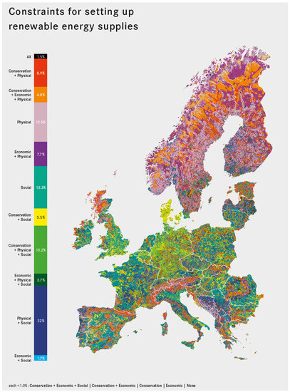
Figure 1.
Contribution of the four motivation groups to the typical exclusions constraints across Europe. Constraints by irradiance and wind speed are not factored into this figure, as distributions of these quantities are well known.
Beyond summary quantities, it can be seen that, despite the broad inclusion of many criteria in each motivation group, a very strong spatial dependence remains. Denmark and Germany, for example, are almost entirely excluded by conservation constraints as well as by social and political exclusions while the same considerations play a minor role in the Nordic countries, where technical economic and physical concerns become prominent. Spain appears to have a similar distribution to Romania and Bulgaria where mountainous ranges lead to conservation, technical economic, and physical motivated exclusions, surrounded by large areas where social and political exclusion areas dominate. There is also extensive variation of motivational contributions within countries. Similar to the Nordic countries, Germany also sees a dependence on physical constraints, although these appear to have a non uniform distribution across the countryside and are particularly present in the south. Furthermore, Switzerland is almost entirely covered by the physically motivated exclusion group, but has pockets of conservation related exclusions and is neatly bisected into a northern and southern region where social and political considerations are also impactful. France and the UK can both be seen to transition between areas where social and political based exclusions play the major role to areas where physical and conservation considerations also become important.
4.2. Independence
Figure 2 shows the result of investigating the independence measure in the form of a heat map, where the constraints have been ordered from left to right for Europe as described in Section 3.3. In the figure, woodlands and agriculture have the most impact across Europe (excluding 51% and 50%, respectively). Following these are, for example, irradiance (43%), protected habitat proximity (35%), connection distance (21%), bird area proximity (20%), and slope threshold (19%). The same results for other countries are shown, but clearly no country shares the same order of constraint independence value to that of Europe. This again emphasizes the point that impacts of various constraints depends heavily on the region in question. River-proximity represents the only legitimate exception to this conclusion, where percentage exclusions are consistently observed between 9% and 13% for all countries. Access distance appears to have a small impact for all countries except in the Nordic regions, suggesting that Europe’s minor road network is extensive. Similarly, irradiance is observed to have a very significant impact across Europe as a whole, but when considered at the country level appears almost binary. With the exception of a few countries, such as Austria and Germany, most countries are excluded completely by the irradiance constraint while others are not affected at all.
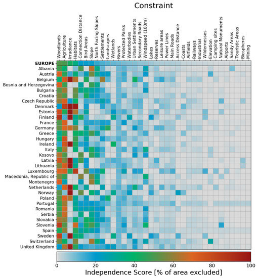
Figure 2.
Independence score by country, where values in red are considered to score better.
There are constraints with a consistently low impact, such as distance from mining sites, touristic areas, camping sites, and protected biospheres, although these results should not be interpreted as these criteria leading to uniformly low exclusions everywhere. Despite the large exclusion buffer of 5 km, airport-proximity also generally results in very little total land exclusion (averaging only 0.8%), with the exception of in Luxembourg where 6% is seen. Slope is an extreme example of regional variability, ranging from 0.04% in The Netherlands to 65% in Albania. Figure 2 shows that the high conservation exclusions seen in Denmark result almost entirely from protected habitats (97%). By comparison, protected habitats are less impactful in Germany (58%), however Germany is also heavily affected by protected landscapes (44%) which together cover the majority on Germany, as observed in Figure 1.
4.3. Overlap and Exclusivity
As described in Section 3.3, computing the percent overlap of a given constraint is a precursor to computing both the overlap as well as the exclusivity measure, therefore these percentages for Europe are shown in Figure 3. Some relationships expressed in this figure are expected and serve to validate the process from a logical consistency perspective. For instance, when given a constraint of high elevations, the resulting exclusions are overlapped almost completely by a constraint based on steep slopes. Similarly, even though the distance to lakes and distance to waterbodies constraint are derived from different data sources, lake exclusions are overlapped completely by those from waterbodies yet the inverse is not true as the waterbody constraint also includes large rivers. Other relationships are also observed, such as, after having excluded areas around all settlements, large portions of areas which would have been excluded by proximities to leisure areas, industrial sites, airports, camping sites, touristic areas, and mining areas are already excluded. However, once again, the opposite is not true, as these constraints have little overlap with a given settlement proximity constraint. In this same way, it is also seen that exclusions from camping sites are significantly overlapped by the exclusion of protected habitats. The access distance constraint is observed to coincide quite well with an irradiance constraint because, as previously mentioned, the access constraint is mostly active in the Nordic countries where one would not expect to find much irradiance. The overlap of protected area designations described previously is also clearly shown by the overlaps of habitats when given the other protected area constraints, where percentage overlap ranges between 60% and 95%.
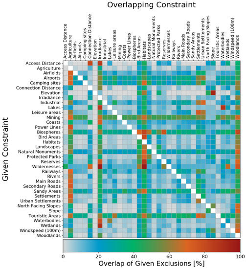
Figure 3.
Constraint overlap for Europe: Percent overlap of a given constraint for a single overlapping constraint. Shown for all pair-wise combination of constraints at the European level.
Figure 4 and Figure 5 display the exclusivity and overlap scores, respectively, at the European and country level. Furthermore, as the scores expressed in these figures are of a relative nature, the values have been scaled to match a range of 0 to 1. By comparing against Figure 2, one can see that constraints which have large independent impact also tend to rank high in both the exclusive and overlapping measure, so it is clear that these constraint measures are not fully independent of each other. For example, the woodland, agriculture, and irradiance constraints have an unfair advantage compared to the others in that they tend to cover so much land that it is highly likely that they will overlap the other constraints while also not being overlapped significantly. The high tendency of the habitats constraint to overlap the other protected areas constraint also causes this constraint to rank highly in the overlap measure, although it does fall slightly in exclusivity. Connection distance and slope are also notable in their consistency considering that they maintain a medium-high score in all three measures. Similarly, distance from mining sites, touristic areas, camping sites, protected biospheres, and airports are once again found to rank low compared to the other constraints. Not all constraints maintain as much of a semi-constant position, however. Both elevation threshold and access distance, for instance, have a medium-low impact, are last in overlap, yet are seen to be much higher in exclusivity. These two exclusions only overlap each other around 15–20%, so the areas these constraints exclude are generally separate from one another.
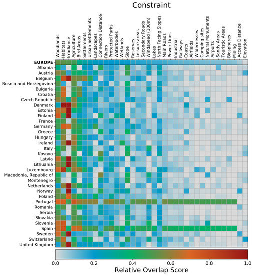
Figure 4.
Overlap scores by country, where values in red are considered to score better. Constraints shown in white did not exclude any areas in the associated region.
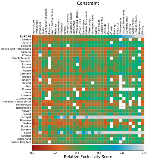
Figure 5.
Exclusivity scores by country, where values in red are considered to score better. Constraints shown in white did not exclude any areas in the associated region.
Once again, it is seen that these comparisons are strongly dependent on the region being investigated. Two clear examples of this are Spain and Portugal. The way in which the various constraints are defined for both of these countries causes in general much higher overlap scores, and by association lower exclusivity scores, in comparison to the other countries. Due to this, results of LE analyses in these countries are likely much less sensitive to the constraints chosen by researchers in comparison to other countries due to the redundant exclusions.
5. Conclusions
This work investigated LE constraint interaction on the European level and illuminated how inclusion of different constraints can have varying effects depending on the constraints in question and the region of study. As this was a general study, the maps and figures presented are not intended to apply to any one specific RES technology, as different technologies will require different constraints. Furthermore, by viewing Figure 1, it should be clear that the country level values displayed in Figure 2, Figure 4 and Figure 5 should not be assumed as constant across these areas, as there will certainly be a large degree of fluctuation within these countries as well. Furthermore, for the sake of simplification in constructing the analysis, only typical constraint threshold values have been used for each of the constraints considered here. Realistically, however, regionally specific values subject to the preferences of local citizens and other stake holders should always be taken into account whenever possible.
Nevertheless, several conclusions can be drawn from the results. Figure 1 shows that, even at a very high level of aggregation, the impact of LE constraints remains highly spatially sensitive. From this, the conclusion can be drawn that general simplifications and tenets regarding LE behavior, such as “including X constraint always results in a Y% reduction in the available land”, are not substantiated across large scales or even, in many cases, within countries. This also supports the notion that improving consistency between LE studies is of high importance as inconsistent methodologies and data practices on top of the clearly highly sensitive nature of this field limits the meaningfulness of comparing or combining LE results from multiple sources. Although ideally all relevant constraints should be considered in an LE analysis, Figure 2, Figure 4 and Figure 5 suggest that constraints based on woodlands, agricultural areas, irradiance and protected habitats are most impactful to LE analyses conducted in Europe as they score highly in all three measures. For this reason, when investigating LE for RES technologies for which some or all of these constraints are relevant, such as for open-field PV or biomass, investigators should emphasize their treatment of these constraints in particular. In the opposite sense, constraints based on distance from mining sites, touristic areas, camping sites, protected biospheres, and airports are found to rank low in all three measures compared to the other constraints. This suggests that these constraints are not of high importance to the outcome of LE studies and can most likely be considered as redundant constraints, meaning they can be altered, or perhaps even excluded, without causing much of a difference. Lastly, the elevation and access distance constraints are examples of constraints which do not tend to exclude much land, but do tend to be unique in their exclusions; thus, they also have the potential to make a significant impact to a final LE result. For this reason the application of these constraints should also be emphasized in the work of LE researchers.
Although this work illuminates interactions between exclusion constraints, one aspect which was not considered is constraint sensitivity. If the threshold value chosen for one or more of these constraints were altered, the extent to which the results would change from those presented here is uncertain. However a full investigation of this dynamic would require a much more detailed investigation than the one presented and discussed here and so is not within the scope of this work. As far as the authors of this work are aware, however, this has not been investigated in broad spatial scopes and is therefore a potential follow-up to this work.
This work and the works it is built upon set the stage for other efforts which can benefit the energy modeling community. For areas that possess equivalent data to that used for the Prior datasets, such as on other continents, it would be interesting to investigate the interdependence of constraints in these contexts and compare the findings against those that were discussed here. Progress in these areas could serve to hone data collection efforts in developing countries and other regions for which data are currently sparse. Most importantly, usage of the GLAES model and Prior dataset can be applied to regions in Europe by local stake holders who have expertise in the areas being investigated to develop exclusion scenarios for onshore wind turbines, open field PV parks, and other RES technologies. If results from these analyses were made available, they would be easily drawn together to formulate a complete picture of European LE as they could easily be recreated, adjusted, or applied in different regional contexts. Such an effort could also serve to identify new criteria that are not already incorporated as Prior datasets. It could also help improve the underlying datasets as locals in these regions would be more able to identify missing or misrepresented features. Finally, it could serve to make energy system design and other such analyses more sensitive to realistic local preferences for RES installation.
References
Author Contributions
D.S.R. proposed the specific research idea, performed data curation, developed the necessary software, performed the formal analysis, prepared the original draft, and implemented the necessary changes during review and editing. M.R. supervised the project, offered direction and interpretation on key aspects, assisted with review and editing, and proposed the overall research topic which includes the idea discussed here. D.S. also proposed the overall research topic, provided direction, performed general project administration, and performed final validation and interpretation of the work before submission.
Funding
This work was supported by the Helmholtz Association under the Joint Initiative “EnergySystem 2050—A Contribution of the Research Field Energy”. Furthermore, it was supported by funding of the Virtual Institute for Power to Gas and Heat by the Ministry of Innovation, Science and Research of North Rhine-Westphalia.
Acknowledgments
Map data are copyrighted by OpenSteetMap contributors and available from https://www.openstreetmap.org. The authors would like to thank the numerous master and bachelor students who contributed to the METIS packages and Christopher Wood for editing this paper. The authors would like to thank the numerous readers of this submission who encouraged us to submit this work for publication.
Conflicts of Interest
The authors declare no conflict of interest.
References
- Baños, R.; Manzano-Agugliaro, F.; Montoya, F.G.; Gil, C.; Alcayde, A.; Gómez, J. Optimization methods applied to renewable and sustainable energy: A review. Renew. Sustain. Energy Rev. 2011, 15, 1753–1766. [Google Scholar] [CrossRef]
- Iqbal, M.; Azam, M.; Naeem, M.; Khwaja, A.S.; Anpalagan, A. Optimization classification, algorithms and tools for renewable energy: A review. Renew. Sustain. Energy Rev. 2014, 39, 640–654. [Google Scholar] [CrossRef]
- Wang, J.J.; Jing, Y.Y.; Zhang, C.F.; Zhao, J.H. Review on multi-criteria decision analysis aid in sustainable energy decision-making. Renew. Sustain. Energy Rev. 2009, 13, 2263–2278. [Google Scholar] [CrossRef]
- Ellabban, O.; Abu-Rub, H.; Blaabjerg, F. Renewable energy resources: Current status, future prospects and their enabling technology. Renew. Sustain. Energy Rev. 2014, 39, 748–764. [Google Scholar] [CrossRef]
- Spiecker, S.; Weber, C. The future of the European electricity system and the impact of fluctuating renewable energy—A scenario analysis. Energy Policy 2014, 65, 185–197. [Google Scholar] [CrossRef]
- Albadi, M.; El-Saadany, E. Overview of wind power intermittency impacts on power systems. Electr. Power Syst. Res. 2010, 80, 627–632. [Google Scholar] [CrossRef]
- Boyle, G. Renewable Electricity and the Grid: The Challenge of Variability; Earthscan: London, UK, 2012; ISBN 1849772339. [Google Scholar]
- Hoogwijk, M.M.; Turkenburg, W.C.; de Vries, H.J.M. On the Global and Regional Potential of Renewable Energy Sources. Ph.D. Thesis, Utrecht University, Utrecht, The Netherlands, 2004. [Google Scholar]
- Huber, M.; Dimkova, D.; Hamacher, T. Integration of wind and solar power in Europe: Assessment of flexibility requirements. Energy 2014, 69, 236–246. [Google Scholar] [CrossRef]
- Klessmann, C.; Held, A.; Rathmann, M.; Ragwitz, M. Status and perspectives of renewable energy policy and deployment in the European Union—What is needed to reach the 2020 targets? Energy Policy 2011, 39, 7637–7657. [Google Scholar] [CrossRef]
- Möller, B. Spatial analyses of emerging and fading wind energy landscapes in Denmark. Land Use Policy 2010, 27, 233–241. [Google Scholar] [CrossRef]
- Loken, E. Use of multicriteria decision analysis methods for energy planning problems. Renew. Sustain. Energy Rev. 2007, 11, 1584–1595. [Google Scholar] [CrossRef]
- Pohekar, S.D.; Ramachandran, M. Application of multi-criteria decision making to sustainable energy planning—A review. Renew. Sustain. Energy Rev. 2004, 8, 365–381. [Google Scholar] [CrossRef]
- Resch, B.; Sagl, G.; Tornros, T.; Bachmaier, A.; Eggers, J.B.; Herkel, S.; Narmsara, S.; Gundra, H. GIS-Based Planning and Modeling for Renewable Energy: Challenges and Future Research Avenues. ISPRS Int. J. Geoinf. 2014, 3, 662–692. [Google Scholar] [CrossRef]
- Holtinger, S.; Salak, B.; Schauppenlehner, T.; Scherhaufer, P.; Schmidt, J. Austria’s wind energy potential—A participatory modeling approach to assess socio-political and market acceptance. Energy Policy 2016, 98, 49–61. [Google Scholar] [CrossRef]
- McKenna, R.; Hollnaicher, S.; Fichtner, W. Cost-potential curves for onshore wind energy: A high-resolution analysis for Germany. Appl. Energy 2014, 115, 103–115. [Google Scholar] [CrossRef]
- Robinius, M.; Otto, A.; Syranidis, K.; Ryberg, D.S.; Heuser, P.; Welder, L.; Grube, T.; Markewitz, P.; Tietze, V.; Stolten, D. Linking the power and transport sectors—Part 2: Modelling a sector coupling scenario for Germany. Energies 2017, 10, 957. [Google Scholar] [CrossRef]
- Samsatli, S.; Staffell, I.; Samsatli, N.J. Optimal design and operation of integrated wind-hydrogen-electricity networks for decarbonising the domestic transport sector in Great Britain. Int. J. Hydrog. Energy 2016, 41, 447–475. [Google Scholar] [CrossRef]
- Sliz-Szkliniarz, B. Assessment of the renewable energy-mix and land use trade-off at a regional level: A case study for the Kujawsko-Pomorskie Voivodship. Land Use Policy 2013, 35, 257–270. [Google Scholar] [CrossRef]
- Tegou, L.I.; Polatidis, H.; Haralambopoulos, D.A. Environmental management framework for wind farm siting: Methodology and case study. J. Environ. Manag. 2010, 91, 2134–2147. [Google Scholar] [CrossRef] [PubMed]
- Ryberg, D.S.; Tulemat, Z.; Robinius, M.; Stolten, D. Geospatial Land Availability for Energy Systems (GLAES). Available online: https://github.com/FZJ-IEK3-VSA/glaes/releases/tag/v1.0.0 (accessed on 14 May 2018).
- Watson, J.J.W.; Hudson, M.D. Regional Scale wind farm and solar farm suitability assessment using GIS-assisted multi-criteria evaluation. Landsc. Urban Plan. 2015, 138, 20–31. [Google Scholar] [CrossRef]
- European Environmental Agency (EEA). Corine Land Cover (CLC) 2012, Version 18.5.1; EEA: Copenhagen, Denmark, 2012. Available online: https://land.copernicus.eu/pan-european/corine-land-cover/clc/2012/view (accessed on 1 April 2017).
- Ryberg, D.S.; Robinius, M.; Stolten, D. Methodological Framework for Determining the Land Eligibility of Renewable Energy Sources. ArXiv, 2017; arXiv:1712.07840. [Google Scholar]
- European Environmental Agency. Europe’s Onshore and Offshore Wind Energy Potential: An Assessment of Environmental and Economic Constraints; EEA: Copenhagen, Denmark, 2009. [Google Scholar]
- Clifton, J.; Boruff, B. Site Options for Concentrated Solar Power Generation in the Wheatbelt; Technical report; Institute for Regional Development, University of Western Australia: Perth, Australia, 2010. [Google Scholar]
- Lanuv, N. Potenzialstudie Erneuerbare Energien NRW; Teil 1-Windenergie; Das Landesamt für Natur, Umwelt und Verbraucherschutz Nordrhein-Westfalen: Recklinghausen, Germany, 2013. [Google Scholar]
- Lütkehus, I.; Adlunger, K.; Salecker, H. Potenzial der Windenergie an Land: Studie zur Ermittlung des Bundesweiten Flächen-und Leistungspotenzials der Windenergienutzung an Land; Umweltbundesamt: Dessau-Roßlau, Germany, 2013. [Google Scholar]
- Vandenbergh, M.; Neirac, F.P.; Turki, H. A GIS approach for the siting of solar thermal power plants application to Tunisia. J. Phys. IV 1999, 9, Pr3-223–Pr3-228. [Google Scholar] [CrossRef]
- Baban, S.M.J.; Parry, T. Developing and applying a GIS-assisted approach to locating wind farms in the UK. Renew. Energy 2001, 24, 59–71. [Google Scholar] [CrossRef]
- Krewitt, W.; Nitsch, J. The potential for electricity generation from on-shore wind energy under the constraints of nature conservation: A case study for two regions in Germany. Renew. Energy 2003, 28, 1645–1655. [Google Scholar] [CrossRef]
- Hansen, H.S. GIS-based Multi-Criteria Analysis of Wind Farm Development. In Proceedings of the 10th Scandinavian Research Conference on Geographical Information Science, Stockholm, Sweden, 13–15 June 2005. [Google Scholar]
- Ma, J.G.; Scott, N.R.; DeGloria, S.D.; Lembo, A.J. Siting analysis of farm-based centralized anaerobic digester systems for distributed generation using GIS. Biomass Bioenergy 2005, 28, 591–600. [Google Scholar] [CrossRef]
- Rodman, L.C.; Meentemeyer, R.K. A geographic analysis of wind turbine placement in Northern California. Energy Policy 2006, 34, 2137–2149. [Google Scholar] [CrossRef]
- Bennui, A.; Rattanamanee, P.; Puetpaiboon, U.; Phukpattaranont, P.; Chetpattananondh, K. Site selection for large wind turbine using GIS. In Proceedings of the PSU-UNS International Conference on Engineering and Environment, Phuket, Thailand, 10–11 May 2007; pp. 561–566. [Google Scholar]
- Tegou, L.I.; Polatidis, H.; Haralambopoulos, D.A. Distributed generation with renewable energy systems: the spatial dimension for an autonomous Grid. In Proceedings of the 47th Conference of the European Regional Science Association, Paris, France, 29 August–2 September 2007; pp. 1731–1744. [Google Scholar]
- Ummel, K.; Wheeler, D. Desert Power: The Economics of Solar Thermal Electricity for Europe; North Africa, and the Middle East Center for Global Development: Washington, DC, USA, 2008. [Google Scholar]
- Lejeune, P.; Feltz, C. Development of a decision support system for setting up a wind energy policy across the Walloon Region (southern Belgium). Renew. Energy 2008, 33, 2416–2422. [Google Scholar] [CrossRef]
- Ramirez-Rosado, I.J.; Garcia-Garridoa, E.; Fernandez-Jimenez, L.A.; Zorzano-Santamaria, P.J.; Monteiro, C.; Miranda, V. Promotion of new wind farms based on a decision support system. Renew. Energy 2008, 33, 558–566. [Google Scholar] [CrossRef]
- Gastli, A.; Charabi, Y.; Zekri, S. GIS-based assessment of combined CSP electric power and seawater desalination plant for Duqum—Oman. Renew. Sustain. Energy Rev. 2010, 14, 821–827. [Google Scholar] [CrossRef]
- Janke, J.R. Multicriteria GIS modeling of wind and solar farms in Colorado. Renew. Energy 2010, 35, 2228–2234. [Google Scholar] [CrossRef]
- Funabashi, T. A GIS Approach for Estimating Optimal Sites for Grid-Connected Photovoltaic (PV) Cells in Nebraska. Master’s Thesis, University of Nebraska-Lincoln, Lincoln, NE, USA, 2011. [Google Scholar]
- Phuangpornpitak, N.; Tia, S. Feasibility study of wind farms under the Thai very small scale renewable energy power producer (VSPP) program. Energy Procedia 2011, 9, 159–170. [Google Scholar] [CrossRef]
- van Haaren, R.; Fthenakis, V. GIS-based wind farm site selection using spatial multi-criteria analysis (SMCA): Evaluating the case for New York State. Renew. Sustain. Energy Rev. 2011, 15, 3332–3340. [Google Scholar] [CrossRef]
- Zhou, Y.; Wu, W.X.; Liu, G.X. Assessment of Onshore Wind Energy Resource and Wind-Generated Electricity Potential in Jiangsu, China. Energy Procedia 2011, 5, 418–422. [Google Scholar] [CrossRef]
- Al-Yahyai, S.; Charabi, Y.; Gastli, A.; Al-Badi, A. Wind farm land suitability indexing using multi-criteria analysis. Renew. Energy 2012, 44, 80–87. [Google Scholar] [CrossRef]
- Grassi, S.; Chokani, N.; Abhari, R.S. Large scale technical and economical assessment of wind energy potential with a GIS tool: Case study Iowa. Energy Policy 2012, 45, 73–85. [Google Scholar] [CrossRef]
- Ouammi, A.; Ghigliotti, V.; Robba, M.; Mimet, A.; Sacile, R. A decision support system for the optimal exploitation of wind energy on regional scale. Renew. Energy 2012, 37, 299–309. [Google Scholar] [CrossRef]
- Sultana, A.; Kumar, A. Optimal siting and size of bioenergy facilities using geographic information system. Appl. Energy 2012, 94, 192–201. [Google Scholar] [CrossRef]
- Aydin, N.Y.; Kentel, E.; Duzgun, H.S. GIS-based site selection methodology for hybrid renewable energy systems: A case study from western Turkey. Energy Convers. Manag. 2013, 70, 90–106. [Google Scholar] [CrossRef]
- Gass, V.; Schmidt, J.; Strauss, F.; Schmid, E. Assessing the economic wind power potential in Austria. Energy Policy 2013, 53, 323–330. [Google Scholar] [CrossRef]
- Gorsevski, P.V.; Cathcart, S.C.; Mirzaei, G.; Jamali, M.M.; Ye, X.Y.; Gomezdelcampo, E. A group-based spatial decision support system for wind farm site selection in Northwest Ohio. Energy Policy 2013, 55, 374–385. [Google Scholar] [CrossRef]
- Effat, H.A. Spatial Modeling of Optimum Zones for Wind Farms Using Remote Sensing and Geographic Information System, Application in the Red Sea, Egypt. J. Geogr. Inf. Syst. 2014, 6, 358–374. [Google Scholar] [CrossRef]
- Szurek, M.; Blachowski, J.; Nowacka, A. Gis-Based Method for Wind Farm Location Multi-Criteria Analysis. Min. Sci. 2014, 21, 65–81. [Google Scholar] [CrossRef]
- Sanchez-Lozano, J.M.; Garcia-Cascales, M.S.; Lamata, M.T. Identification and selection of potential sites for onshore wind farms development in Region of Murcia, Spain. Energy 2014, 73, 311–324. [Google Scholar] [CrossRef]
- Schallenberg-Rodriguez, J.; Pino, J.N.D. Evaluation of on-shore wind techno-economical potential in regions and islands. Appl. Energy 2014, 124, 117–129. [Google Scholar] [CrossRef]
- Latinopoulos, D.; Kechagia, K. A GIS-based multi-criteria evaluation for wind farm site selection. A regional scale application in Greece. Renew. Energy 2015, 78, 550–560. [Google Scholar] [CrossRef]
- Tsoutsos, T.; Tsitoura, I.; Kokologos, D.; Kalaitzakis, K. Sustainable siting process in large wind farms case study in Crete. Renew. Energy 2015, 75, 474–480. [Google Scholar] [CrossRef]
- Höfer, T.; Sunak, Y.; Siddique, H.; Madlener, R. Wind farm siting using a spatial Analytic Hierarchy Process approach: A case study of the Städteregion Aachen. Appl. Energy 2016, 163, 222–243. [Google Scholar] [CrossRef]
- Atici, K.B.; Simsek, A.B.; Ulucan, A.; Tosun, M.U. A GIS-based Multiple Criteria Decision Analysis approach for wind power plant site selection. Util. Policy 2015, 37, 86–96. [Google Scholar] [CrossRef]
- Hernandez, R.R.; Hoffacker, M.K.; Field, C.B. Efficient use of land to meet sustainable energy needs. Nat. Clim. Chang. 2015, 5, 353–358. [Google Scholar] [CrossRef]
- Trieb, F. Expert System for Solar Thermal Power Stations; Institute of Technical Thermodynamics (DLR): London, UK, 2001. [Google Scholar]
- European Environmental Agency. Digital Elevation Model over Europe (EU-DEM). Available online: https://www.eea.europa.eu/data-and-maps/data/eu-dem (accessed on 1 April 2017).
- UNEP-WCMC and IUCN. Cambridge, UK. Protected Planet: The World Database on Protected Areas (WDPA). Available online: www.protectedplanet.net (accessed on 1 April 2017).
- GEODATA, GISCO, Eurostat. Clusters: Urban 2011. Available online: http://ec.europa.eu/eurostat/web/gisco/geodata/reference-data/population-distribution-demography/clusters (accessed on 1 April 2017).
- OpenStreetMap Contributors. OpenStreetMap. Available online: https://www.openstreetmap.org (accessed on 1 April 2017).
- GEODATA, GISCO, Eurostat. Transport Networks: Airports 2013. Available online: http://ec.europa.eu/eurostat/web/gisco/geodata/reference-data/transport-networks (accessed on 1 April 2017).
- Messager, M.L.; Lehner, B.; Grill, G.; Nedeva, I.; Schmitt, O. Estimating the volume and age of water stored in global lakes using a geo-statistical approach. Nat. Commun. 2016, 7, 13603. [Google Scholar] [CrossRef] [PubMed]
- GEODATA, GISCO, Eurostat. Hydrography (LAEA). Available online: http://ec.europa.eu/eurostat/web/gisco/geodata/reference-data/elevation/hydrography-laea (accessed on 1 April 2017).
- Technical University of Denmark. DTU Global Wind Atlas 1 km Resolution. Available online: https://irena.masdar.ac.ae/gallery/#map/103 (accessed on 1 April 2017).
- World Bank Group. Global Solar Atlas. Available online: http://globalsolaratlas.info/ (accessed on 1 April 2017).
- GDAL Development Team. GDAL—Geospatial Data Abstraction Library; Version 2.1.1; Open Source Geospatial Foundation: Chicago, IL, USA, 2017. [Google Scholar]
- Jones, E.; Oliphant, T.; Peterson, P. SciPy: Open Source scientific tools for Python. Comput. Sci. Eng. 2017, 9, 10–20. [Google Scholar]
- Dudley, N. Guidelines for Applying Protected Area Management Categories; International Union for Conservation of Nature (IUCN): Gland, Switzerland, 2008. [Google Scholar]
- Directive, E.B. Directive 2009/147/EC of the European parliament and of the Council of 30 November 2009 on the conservation of wild birds (codified version). Off. J. L 2009, 20, 7–25. [Google Scholar]
- Directive, H. Council Directive 92/43/EEC of 21 May 1992 on the conservation of natural habitats and of wild fauna and flora. Off. J. Eur. Union 1992, 206, 7–50. [Google Scholar]
© 2018 by the authors. Licensee MDPI, Basel, Switzerland. This article is an open access article distributed under the terms and conditions of the Creative Commons Attribution (CC BY) license (http://creativecommons.org/licenses/by/4.0/).