Article

Application of Hybrid Meta-Heuristic Techniques for Optimal Load Shedding Planning and Operation in an Islanded Distribution Network Integrated with Distributed Generation

1
Power Electronics and Renewable Energy Research Laboratory (PEARL), Department of Electrical Engineering, University of Malaya, Kuala Lumpur 50603, Malaysia
2
Department of Electrical Engineering, University of Malaya, Kuala Lumpur 50603, Malaysia
3
Department of electrical engineering, Quaid-e-Awam University of Engineering Science and Technology, QUEST, Nawabshah, Sindh 67450, Pakistan
*
Author to whom correspondence should be addressed.
Energies 2018, 11(5), 1134; https://doi.org/10.3390/en11051134
Submission received: 25 March 2018 / Revised: 20 April 2018 / Accepted: 1 May 2018 / Published: 3 May 2018

Abstract

:
In a radial distribution network integrated with distributed generation (DG), frequency and voltage instability could occur due to grid disconnection, which would result in an islanded network. This paper proposes an optimal load shedding scheme to balance the electricity demand and the generated power of DGs. The integration of the Firefly Algorithm and Particle Swarm Optimization (FAPSO) is proposed for the application of the planned load shedding and under frequency load shedding (UFLS) scheme. In planning mode, the hybrid optimization maximizes the amount of load remaining and improves the voltage profile of load buses within allowable limits. Moreover, the hybrid optimization can be used in UFLS scheme to identify the optimal combination of loads that need to be shed from a network in operation mode. In order to assess the capabilities of the hybrid optimization, the IEEE 33-bus radial distribution system and part of the Malaysian distribution network with different types of DGs were used. The response of the proposed optimization method in planning and operation were compared with other optimization techniques. The simulation results confirmed the effectiveness of the proposed hybrid optimization in planning mode and demonstrated that the proposed UFLS scheme is quick enough to restore the system frequency without overshooting in less execution time.

1. Introduction

Recently, a large number of distributed generation (DG) has been installed in power system networks around the world. For instance, 18% of Europe’s electricity is based on DGs sources, such as wind power and hydro [1]. Malaysia is also seeking to raise its renewable energy usage from 6% to 11% in the period between 2011–2020 [2]. The benefits of integration of DG include improved load balance, voltage profile, energy efficiency and reliability.
The concept of microgrid allows for the integration of more DGs, such as wind turbines, solar PV systems, fuel cells, and microgas turbines, storage devices such as flywheels, supercapacitors, and batteries in existing distribution networks. Simultaneously, the microgrids can feed the local loads which include both critical and noncritical loads. In practice, the control and management of MG are centrally conducted by a microgrid central controller (MGCC) which is installed in the medium-/low-voltage (MV/LV) substation [3]. Generally, a MG operates in two modes; grid-connected and islanding. The MGCC is regarded the administrator of the MG hierarchical control systems, which has the ability to manage economic issues and control functionalities. In the grid-connected mode, the main grid and local DGs in MG can dispatch power to the loads as per the requested demand. In this case, the MGCC provide power references for DGs within the MG, while, the MV grid sets the root mean square voltage, to include a DGs to only generate currents. In that case, the DGs’ inverters control is known as “Active and Reactive power control (PQ control)”. On the other hand, the MG islanding mode could be due to an intentional disconnection from the MV grid that was ordered to for maintenance purposes or from a forced disconnection caused by a fault in the MV network as the voltage dips. Hence, the frequency and voltage in the MG must be kept within the allowable limits by the MG DGs. In order for it to do this, a DG can implement a voltage source inverter with a frequency set point and an inner loop of reference voltage to compensate for the imbalance of power between loads and MG power. That DG is known as a “master source” and operates on VF mode. Contrarily, the other DGs in MG are known as “slave sources” and operate on PQ mode. It should be pointed out that the MGCC sends the PQ references to slave DGs to generate real power in order to avoid overloading inverters and to ensure that load changes are properly controlled. In the context of isolated microgrids, paper [4] developed a coordinated control strategy for managing the active power reserve.
When the main grid is connected to a distribution network, the energy production closely matches energy consumption. However, when the islanded network is formed, it may lead to an imbalance between the generation and load demand in the power system operation. Consequently, it could lead to frequency and voltage instabilities, overloading in the line, and in the worst-case scenario, power system blackouts [5,6].
Nowadays, due to increasing integration of DGs with the power systems, power systems have become very complex. For that, an intelligent load shedding scheme is needed to overcome the traditional load shedding techniques which incapable to offer efficient load shedding in order to shed the optimal load and maintain power system stability. Accordingly, several intelligent load shedding schemes have been proposed. The optimal of load shedding scheme based on Artificial Neural Network (ANN) for an isolated power system was proposed in [7]. In this technique, the inputs of ANN include total generation, total load demand, and the frequency drop rate, while its output is the minimum amount of load shedding. A comparative study was carried out to prove that the proposed load shedding is faster than the conventional technique. Also, an ANN-based load shedding technique was applied on Taiwan’s power system to increase the reliability [8]. The results confirmed that the ANN-based load shedding technique is suitable for real-time applications due to shedding the exact amount of load. Moreover, [9] suggested an optimal load shedding based on the ANN technique and they applied it on a 39-bus New England power. The results showed that the proposed technique is capable of shedding an optimal load to stabilize the power system. The authors in [10] suggested a new fuzzy Under Frequency Load Shedding (UFLS) technique for an islanded microgrid. This technique is dynamic and robust towards regulating frequencies in different cases. The authors in [11] proposed a new fuzzy logic based UFLS technique for an islanded distribution network that is able to restore the frequency as soon as possible. It uses frequency, the rate of change of frequency, and load priority to do this. An UFLS technique based on the forecast of the minimum frequency was proposed in [12]. In this technique, the system frequency samples are taken post-disturbance; then, the Particle Swarm Optimization (PSO) method is used to forecast the minimum frequency and shed the required loads. Moreover, Genetic Algorithm (GA) is also applicable in certain load shedding problems. The authors in [13] proposed a genetic algorithm application for the load shedding technique. It was verified on an IEEE 30-bus system. Another GA-based load shedding technique that can minimize the amount of load shed was proposed in [14]. A comparative simulation study of the proposed and conventional techniques was performed to confirm the ability of the GA-based technique in shedding optimal loads.
An optimal load shedding technique based on the PSO method was reported in [15] to determine the maximum loading point. The technique was verified on an IEEE 14-bus system. A comparative simulation study between PSO and GA methods was also performed, and it was confirmed that the UFLS technique based on the PSO method is able to find the optimal solution more quickly compared with the genetic algorithm method [16] used the particle swarm-based-simulated annealing optimization method to provide long-term voltage stability. The most important feature of the proposed method is its capability to determine the global optimum solution within a few iterations.
Commonly used optimization techniques such as Evolutionary Programming (EP) algorithms and Genetic Algorithm (GA) are limited due to their computational time needs and premature convergence. These limitations may result in a non-optimal load shedding scheme. Accordingly, this study integrates between two algorithms to obtain an effective optimization algorithm known as the Firefly Algorithm-Particle Swarm Optimization (FAPSO).
The Firefly algorithm (FA) is a newly designed algorithm that mimics the flashing technique of fireflies. A detailed explanation and formulation of the firefly algorithm will be given in Section 2.2.3. A. FA has one demerit when finding a solution, it is sometimes trapped in a local optimum solution [17]. The firefly algorithm does not have a technique to remember the previous best solution of each firefly because the parameters in the firefly algorithm are fixed. Thus, it makes the fireflies move without taking into consideration its previous better solution. Moreover, FA also encounters some difficulties such as premature convergence and obtaining better solutions. On the other hand, the PSO algorithm is regarded as more common optimization algorithms and is applicable for many types of optimization problems. The PSO is a computational technique that depends on the movement of the swarm to determine the optimal solution in the search space. The swarm movement in the PSO algorithm in the search space takes its inspiration from a group of birds or bees. The major advantages of the PSO algorithm are simple context, easy implementation mechanism, and minimal storage requirements [18]. However, the PSO often faces some problems such as taking a long time to converge to optimal.
According to the previous explanation, despite the privileges of FA and PSO algorithms, they have some drawbacks, and in order to mitigate/minimize them, the two algorithms can be merged/combined. The main goal of the proposed hybrid algorithm is realizing both local search using the flashing behaviour operation of Firefly in FA, and global search via PSO optimization. Therefore, it can be achieved a balanced search between exploration and exploitation. This hybridization between FA and PSO serve the load shedding technique to find the optimum solution with less number of iteration in planning load shedding. Moreover, FAPSO aims to play an important role in reducing the execution time of load shedding operation in real time application.
The UFLS scheme is used to prevent a frequency instability in a distribution network that is caused by power imbalance. In order to restore power balance, the UFLS scheme curtails a specific amount of loads when the amount of reserve power is inappropriate to compensate a power imbalance. It should be pointed out that a quick frequency decline that is caused by a generation loss or large excess load will take place due to the inadequate spinning power reserve and a small system inertia. The UFLS scheme is carried out to maintain the system frequency within allowable limits by keeping a balance of electricity between a power generation and load demand [19]. There are two main types of UFLS schemes; conventional and adaptive UFLS schemes. The conventional UFLS scheme is considered the most common load shedding technique implemented by power utilities [20,21], where it curtails a fixed amount of loads at certain frequency thresholds without taking into account voltage dip, frequency decline, and disturbance location [22]. However, this technique is unable to shed the correct amount of power deficit [23], and therefore, in practice, the conventional UFLS scheme may lead to the removal of load quantity at levels lower/higher than the amount of power deficit, which could result in overshooting/undershooting in system frequency, respectively.
In the worst-case scenario, the frequency instability will cause power system blackout due to either over-shedding or under-shedding loads in the system. To solve this problem, an adaptive UFLS was proposed, which employs the system frequency, the first derivative of system frequency and generator swing equation in order to estimate a power deficit [23,24,25]. In adaptive UFLS scheme, the amount of imbalance power is taken into consideration in order to determine the amount of curtailed loads. In addition, the load selection of load shedding process depends on a specific priority ranking of loads. The adaptive UFLS has been improved by utilizing the spinning reserve in the generators to minimize the total load shedding in [24]. In references [26,27], the adaptive UFLS technique proposed for islanding distribution network curtailed lower loads relative to its conventional counterpart. However, this technique reported a flaw taking place in the amount of load shed when the unoptimal amount of load that was curtailed resulted in an overshooting frequency. Recently, researchers started using artificial intelligence methods for load shedding techniques. The authors in [28] proposed a new fuzzy UFLS scheme for an islanded microgrid. This scheme demonstrated dynamics and robustness in regulating frequencies in multiple cases. However, the system’s frequency still overshoots. Other intelligent UFLS schemes presented in [29,30,31] also showed that the amounts of loads being shed remain not optimal in certain cases. Over-shedding is caused by fixed priorities in the load shedding process. For this reason, Laghari et al. [24] proposed a new UFLS technique, which assumes some flexibility in load priority, making it possible to shed the optimal combination of loads with minimum error. The UFLS technique proposed in [24] is capable of restoring the system’s frequency to its nominal value without overshooting/undershooting during the islanded distribution network. However, this technique suffers from long computational time, since all possible load combinations needs to be considered. For this reason, the authors chose only six random priority loads. For that purpose, the adaptive UFLS also needs another technique to select the loads that will be shed to realize an optimal load curtailment. For that, the FAPSO optimization is proposed to select the loads that should be shed which realized the optimum load shedding with a minimum number of iterations.
This paper focuses on planning and operation of load shedding in the islanded distribution network, which is based on the proposed FAPSO optimization. FAPSO optimization is used as an optimization tool for evaluating the planning optimal load shedding, meanwhile, the Stability Index (SI) is used in order to detect the buses that are most sensitive to voltage collapse in any operating point in the distribution system. It is suggested that SI is applied on combines weighted objectives into a single objective function with the amount of Megawatt (MW) for remaining load in the system. Moreover, the proposed FAPSO optimization method has been compared under islanded distribution network with PSO, FA, Evolutionary Programming (EP) and Gravitational Search Algorithm (GSA). The main goal of comparison is to determine the best algorithm for applying load shedding scheme. This determination performs by measuring the accuracy of the final solution and convergence speed for maximizing load remaining and improving the lowest Stability Index (SI) value. On the other hand, the FAPSO optimization is also used in UFLS scheme in order to select appropriate buses for load shedding. This selection is performed based on achieving the minimum error between the sum of the best combination loads to be shed and the total amount of required load shedding. To assess the capabilities of the proposed method, simulations were carried out using Matlab software on an IEEE 33-bus radial distribution system and PSCAD software on part of the Malaysian distribution network with different types of DGs by considering various scenarios.
This paper is organized in the following manner: Section 2 details the proposed optimal load shedding planning. Section 3 details the proposed UFLS scheme using FAPSO algorithm. Section 4 will discuss modelling of IEEE 33-bus radial distribution network and determine the types, locations, and amount of DGs in the test system and load profile used in the test system. Section 5 presents the simulation results and discusses the proposed FAPSO based on planning load shedding scheme and its comparison with FA, PSO, EP and GSA algorithms. Section 6 presents real test system to verify the proposed UFLS scheme. Section 7 presents and discusses the simulation results of proposed UFLS scheme and compare it with other schemes. The conclusions of the work will be detailed in Section 8.

2. Optimal Load Shedding Planning

This section presents the tools that used in optimal load shedding planning in order to maximize remaining loads and improve voltage profile within acceptable limits.

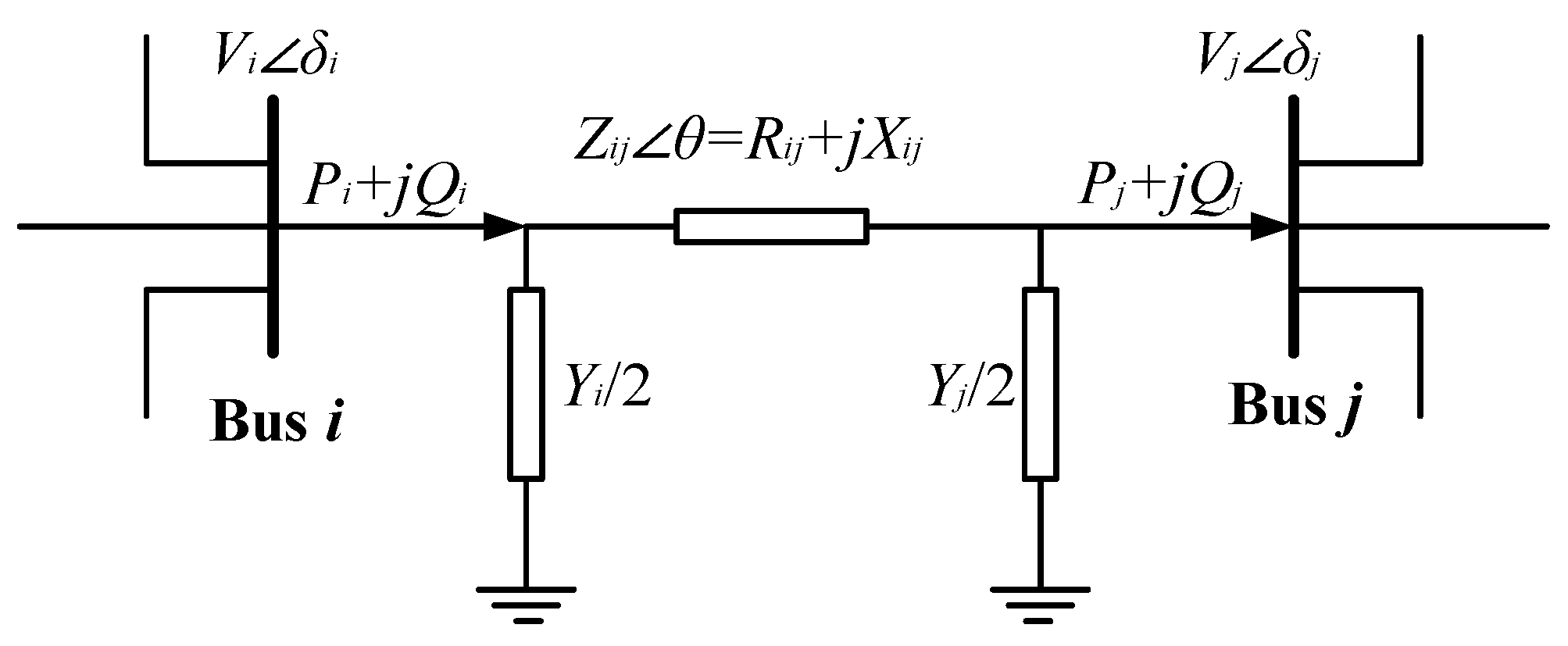
2.1. Voltage Stability Index

This section describes voltage stability index formulation, referred to as the SI, which is suitable for a distribution network and used in the load shedding scheme. SI was proposed in [32] to determine the weakest bus in a network that could lead to voltage instability when the load increases. To understand the SI, Figure 1 shows two buses in a power system model and its parameters. The line VSIs indicates the status of stability at the end of the line (received bus). Meanwhile, the bus VSIs indicates the status of bus stability. Due to the fact that SI can be utilized to evaluate the critical loads in an islanded system, SI can be included in the optimization problem of load shedding schemes. Therefore, this research integrates the SI in the planning load shedding scheme in order to affect a more reliable solution.
The symbols seen in Figure 1 are: Vi, Vj: voltage magnitude at the sending (i) and receiving (j) buses, respectively. Pi, Qi: active and reactive power at the sending bus. Pj, Qj: active and reactive power at the receiving bus. δi, δj: voltage angle at the bus i and bus j, respectively. Y: line shunt admittance. R, X, θ: line resistance, line reactance and line impedance angle. The line impedance amplitude is Z. The shunt admittances Y are neglected for simplicity.
The value of the index is given by:
S I = | V i | 4 [ 4 ( P j X i j Q i R i j ) 2 4 ( P j R i j Q i X i j ) 2 ] | V i | 2 0
where SI is the voltage stability index; Vi is the sending bus voltage in pu; Pj and Qj are the active and reactive load at the receiving end in pu, respectively; Rij and Xij are the resistance and reactance of the line i-j in pu.
In order to realize a more stable radial distribution networks, the value of SI should be closer to one for all buses. When the SI value reaches zero, it indicates the voltage collapses in the bus carring this value [32,33,34]. Therefore, to avoid the possibility of voltage collapse; the SI of all nodes should be maximized. In the proposed algorithm, SI values will be calculated for each bus in the network and sorted from the lowest to the highest values. The bus with the lowest value of SI will be considered in the fitness function.

2.2. Proposed Load Shedding Scheme

2.2.1. Formulation of Objective Function

In this study, the optimization aims to maximize both the sum of load remaining after the load shedding process and the voltage profile of distribution network. For achieving a good fitness value of the objective function for this paper, a combining weighted objectives into a single objective method of has been chosen. This means, the two objectives can be virtually separated, by giving each of them its specific weight in the optimization process. In order to realize that, the objective function (f) needs to be formulated to minimize objective function one (f1) and objective function two (f2) in the following manner:
Minimize   f = w 1 f 1 + w 2 f 2
where:
w 2 = 1 w 1
f 1 = A × ( 1 T = 1 L P r e m a i n , T )
f 2 = 1 S I s y s t e m
where w1 and w2 are fixed positive weight values, w1 is chosen is in the range of [0, 1], and it used in the optimization algorithm to minimize the objective function of and determine the priority of two terms f1 and f2. T represents the load bus number. L represents the number of the load buses in the distribution network. A is a reference value to make f1 unit-less value to be able to add to the f2 term, and this value is equal to 1 MW in this study. Premain represents the remaining loads after load shedding process for each bus. SIsystem represents the lowest value of SI from all values of SI for load buses. The lowest value of SI refers to the weakest bus in the distribution network. This value is selected to improve all the voltage buses in distribution network within allowable limits during a load shedding process.
In order to select the appropriate weightage values in Equation (2), a searching process is performed by changing the value w1 from 0 to 1 with a step size of 0.1. This is done to determine the importance of each weightage set (wset) towards the objective function. To assess the performance of each weightage set, the Least Average Value (LAV) is formulated to be a performance index. The LAV is calculated by:
L A V = f 1 , w s e t , α minimum   ( f 1 , o v e r a l l ) minimum   ( f 1 , o v e r a l l ) + f 2 , w s e t , α minimum   ( f 2 , o v e r a l l ) minimum   ( f 2 , o v e r a l l ) 2
where wset,α represent f1 and f2 values at weightage set α (where α = 1, 2, …, 11). f1,overall and f2,overall represent the overall f1 and f2 values. The performance index based on LAV (ηLAV) is expressed as:
η L A V = 1 L A V
It should be pointed out, the aim of the ηLAV is estimating the least point which represents the minimum value of both objective functions (f1 and f2) simultaneously. Therefore, by determination the largest value of ηLAV, proper weightage values can be determined, leading to the maximum remaining load in the distribution network with high value of SI, simultaneously.

2.2.2. Constraints

Equality/inequality constraints that should be fulfilled for the load shedding are:
(A) The equality in power flow
The total power generated by DGs should be equal to the total load and total loss in the network after load shedding:
Ω = 1 D P D G , Ω = Τ = 1 L P L o a d , Τ + P L o s s
Ω = 1 D Q D G , Ω = Τ = 1 L Q L o a d , Τ + Q L o s s
where PDG and QDG are the active and reactive powers generated from the DG, respectively. Ω represents the DG number. D represents the total numbers of the DG units in the distribution network. PLoad and QLoad are active and reactive loads in the distribution network after load shedding optimization for each bus, respectively. T represents the load bus number. L represents the total numbers of load buses in the distribution network. PLoss and QLoss are the total active and total reactive losses in the distribution network after load shedding optimization, respectively.
(B) Limitations of bus voltage
The voltage magnitudes at all buses after load shedding should be within permissible limits, as shown below:
V i , min V i V i , max
where Vi is a voltage for i bus, and Vi,min, and Vi,max range between ±10% of its nominal value, respectively.
(C) Limitations on the amount of load shed at each bus
The allowable amount of load shedding for any selected load bus should be in limited priority value. In other words, the minimum value of load remaining after load shedding at each bus is not less than the set value, as follows:
S i , p r i o r i t y S i , a f t e r _ s h e d d i n g S i , b e f o r e _ s h e d d i n g
where Si,priority is the minimum amount of load power that must be maintained for load bus number i. Si,after_shedding and Si,before_shedding represent the load power after and before applying load shedding process, respectively.
(D) The boundary of the output power of DG
After islanding is formed, the DGs should work at the maximum output power (PDG,max) to compensate a part of the shortage power in the distribution network. The limit of generator power (PDG) is given as:
P D G = P D G , max

2.2.3. Load Shedding Optimization Algorithm

The proposed strategy uses the power flow analysis to achieve the optimal load shedding with improving the voltage profile. This work solves the optimal load-shedding problem using the hybrid FA and PSO (FAPSO) technique and compares its’ results with each of FA, PSO, EP and GSA algorithms. A detailed description of the FA, PSO and proposed algorithms are presented in the following section, while EP algorithm was described in detail in [35,36] and GSA algorithm was detailed in [37].
(A) Firefly algorithm (FA)
FA is a recent nature-inspired meta-heuristic optimization method. This algorithm was designed by Yang in 2007 as mentioned in [38]. Fireflies are small insects, which are capable of producing light to attract other fireflies. They release light flashes as a signal system. There is an inverse relationship between light intensity attraction ‘I’ of fireflies and the distance ‘r’. Hence, most fireflies are visible only up to several hundred meters. To execute this algorithm, the fitness function is articulated based on the fluorescence light behaviour of fireflies. For simplicity, it is imagined that light intensity attractiveness of firefly is determined by its brightness ‘I’, which is in turn connected to the fitness function. The main feature of FA is based on the flashing characteristics of the firefly [39]. The brightness ‘I’ of a firefly can be selected as Ir proportional to the fitness for a maximization problem. So, the Ir varies according to the well-known inverse square law as shown in Equation (13):
I r = I s r 2
where Is is the intensity at the source r
When the brightness ‘I’ of a firefly increased, the fireflies’ attractiveness, β, will increase, and vice versa. Thus, the attractiveness of the fireflies is strongly proportional to their brightness. Fireflies attractiveness, β, can be defined as:
β ( r ) = β 0 e ( γ   r 2 )
where β0 is the attractiveness at r = 0; γ is the coefficient of the light absorption; r is the distance between any two fireflies y and z at firefly (fy) and firefly (fz), respectively.
The Cartesian distance can be expressed as follows:
r y z = k = 1 d ( f y , k f z , k ) 2
where, fy,k. fz,k are the kth component of the spatial coordinate fy and fz of the kth firefly, respectively. d is the dimensionality of the problem. The movement of fireflies, where new firefly y,k ( f y , k t + 1 ) is attracted to previous firefly z,k ( f z , k t ) is determined by:
f y , k t + 1 = f y , k t + β 0 e γ   r y z 2 ( f z , k t f y , k t ) + α ( r a n d 0.5 )
where the second term is caused by the attraction, while the third term, governed by the randomization parameter α, is responsible for the insertion of certain randomness in the path followed by the firefly, and rand is a random number between 0 and 1.
(B) Particle Swarm Optimization (PSO)
PSO is another meta-heuristic method used by most researchers for the optimization problem. It was originally proposed by Eberhart and Kennedy in 1995 [40]. The major principle of PSO is created according to the behaviour of birds or fish searching for food. The advantage of using PSO over other optimization techniques is its simplicity and the fact that it requires very little adjustment to a few set parameters. Due to this fact, PSO has been widely used in a variety of applications.
Let a number of k particles in a swarm be initialized with positions xtk = (xt1, xt2, xt3, …, xtk) and velocities vtk = (xt1, xt2, xt3, …, xtk), and the fitness is calculated based on particle positional coordinates as the input values. Then, the particles are moved into new positions using the equations below:
x k t + 1 = x k t + v k t + 1
v k t + 1 = w v k t + c 1 r 1 ( P b e s t x k t ) + c 2 r 2 ( G b e s t x k t )
w = w max w max w min i t e r max × i t e r
where, x k t and x k t + 1 are the current position of the particle k at iteration t and t + 1, respectively; v k t and v k t + 1 are the current velocity of the particle k at iteration t and t + 1, respectively; c1 and c2 are the weighting factors; r1 and r2 are a random number between 0 and 1; wmax and wmin are the maximum and the minimum weight of the initial, respectively; iter and itermax are the current iteration number and the maximum iteration number, respectively. Each particle updates its position and velocity based on its own searching experience called Pbest, and on the experience from the other particle called Gbest.
(C) Proposed Method: Hybrid of FA and PSO (FAPSO) Optimization
In this method, the capability of the FA is integrated with the PSO to increase its chance for not being trapped in a local solution and increase speed convergence. The FAPSO share similar procedures to that of the FA. However, the movement of fireflies in FAPSO is modified, where new firefly ( f y , k t + 1 ) is randomly mutated by:
f y , k t + 1 = f y , k t + β 0 e γ   r y z 2 + c 1 r 1 ( f G b e s t , k t f y , k t ) + α ( r a n d 0.5 )
Figure 2 illustrates the flowchart for the implementation of FAPSO method.
In the proposed method, the light intensity attraction step of each particle is mutated by a modified mutation function in the FAPSO operator. For that, each particle is randomly attracted towards the Gbest position in the same population. Local search in different regions is implemented by the attractiveness step of the FA algorithm. The FAPSO algorithm outperforms the FA and PSO algorithms in solving the optimization problems by using the flashing behaviour of fireflies.

2.2.4. Procedure

The implementation of FAPSO algorithm to optimal load shedding problem can be shown in Figure 3.

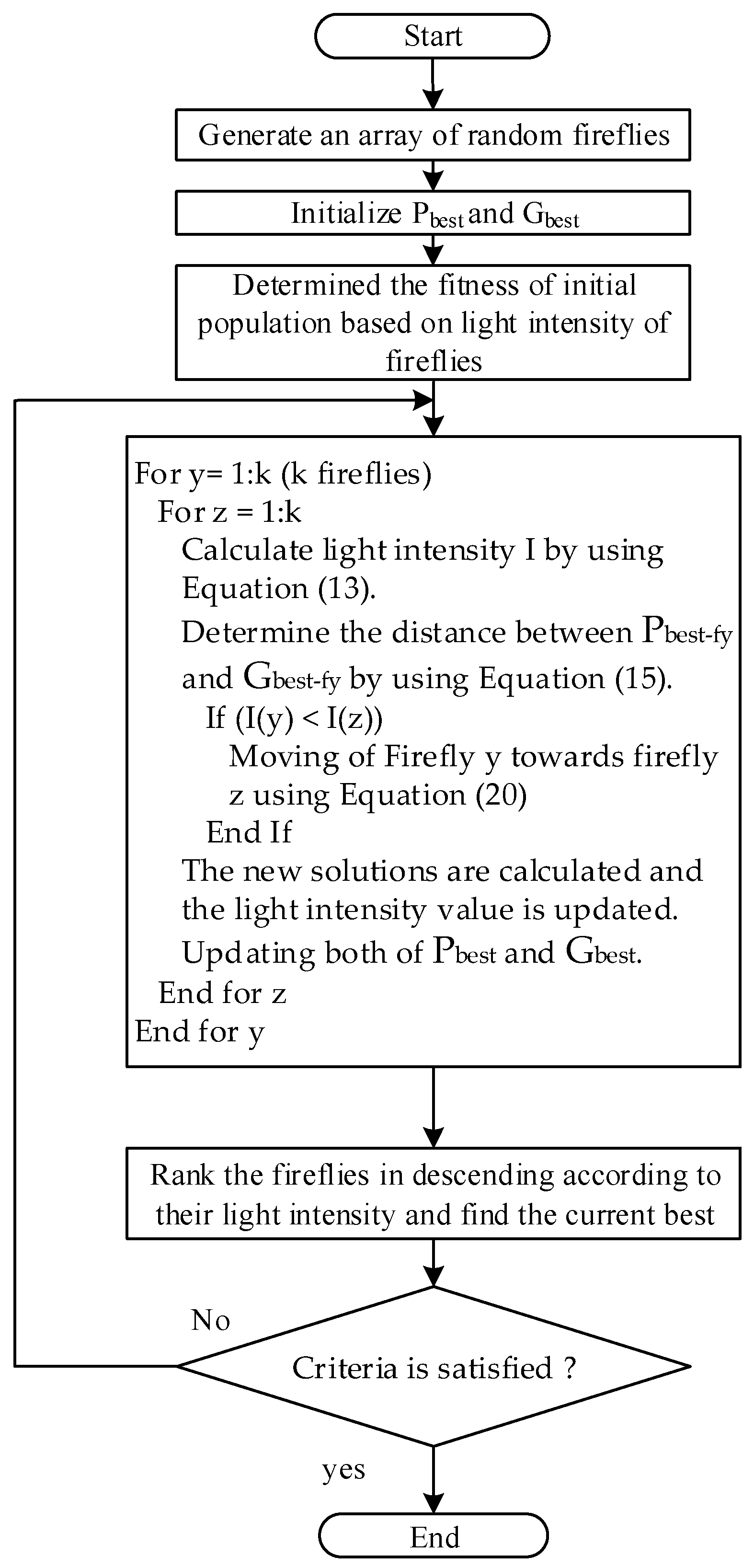
3. Proposed UFLS Scheme Using FAPSO Algorithm

The UFLS scheme will only activate its process when it receives a tripping signal from an incoming grid substation breaker, indicating the formation of islanding. The amount of power deficit as a result of the formation of islanding is equal to power incoming grid to the distribution network. On the other hand, the amount of power deficit during islanding is calculated based on the rate of change of frequency (ROCOF). It is worth mentioning that the frequency of the centre of inertia (COI) is considered in UFLS scheme whenever there is more than one generator in the islanded distribution network. The center of inertia frequency, in Hertz, can be determined using Equation (21):
f C O I = i = 1 N H i f i / i = 1 N H i
where N is the number of connected generators; Hi is the inertia constant of each generator in seconds; fi is the frequency of each generator in Hertz. In this study, the value of 47.5 Hz and 52.5 Hz are the limitations of system frequency. It should also be pointed out that the protection devices are immediately activated to disconnect all DGs, when the value of system frequency declines under 47.5 Hz or exceeds over 52.5 Hz, which results in a blackout.
In order to minimize the amount of load to be shed, the spinning reserve of the system can be used. It should be pointed out that the spinning reserve of the system relies on the generators’ capacity. The value of the total spinning reserve (TSR) of the system can be determined using Equation (22):
T S R = i = 1 N M G C i i = 1 N A G P i
where N is the number of connected generators; MGCi is the maximum generation capacity of ith generator; AGPi is the actual generated power of ith generator.
When the load shedding controller senses any imbalance between the generated and demanded active power in the system during islanding mode, it calculates the power deficit in the system in two different strategies:
(i)
Event-based strategy—when one or more of generator supply like Renewable Energy Source (RES) are disconnected from distribution network and/or the decreasing in output power generated by RESs (such as wind turbine and Photovoltaic).
(ii)
Response based strategy—when suddenly load increased in the islanded distribution network.
In the first strategy, it is estimated the power deficit by detecting the status of generator breaker and recording the last generated power output before the outage as illustrates in Equation (23):
P d e f i c i t = j = 1 M P disconnected   Source
where Pdeficit is the imbalance power during islanding mode (including power loss), per-unit, j = 1 M P d i s c o n n e c t e d   Source is the sum of output power for tripped generators, per unit, and M is the number of trip generators. It can be noted from the last equation, the estimated power deficit that resulted from tripping generator equals to the total loss of generated power in the system. To calculate the power deficit for RESs can be used Equation (24):
P d e f i c i t = P R E S , 0 P R E S
where PRES,0 is the total output power generated by RESs at the source of RESs change event (like wind speed or sun radiation); and PRES is the total output power generated by RESs at 0.01 ms after the source of RESs change event.
The second strategy is based on the dfCOI/dt. When there is a change in the rate of frequency caused by load increment event, the power deficit can be calculated based on a power swing equation:
P d e f i c i t = 2 × d f C O I d t × i = 1 N H i f n
where Pdeficit is the imbalance power during islanding mode per-unit; dfCOI/dt is the rate of change of center of inertia frequency at first disturbance in the system, Hz/s; Hi the inertia constant of ith connected generator; N is the number of connected generators; fn is the rated value of frequency, Hz.
The primary frequency control of DGs is activated when the center of inertia frequency reached 49.8 Hz to enhance the reduction in the declination in the frequency of the system [41]. This value can be adjusted according to the needs of the protection. To get better system frequency response and restore the frequency to its referenced value, the proper amount of load that should be shed from the system can be determined based on the following equation:
TLSA = PdeficitTSR
where TLSA is the total load shed amount. After the controller determines the amount of loads that can be shed from the system, the next step is finding the best combination of load buses that are to be disconnected from the network. The problem of determining the optimal combination of load shedding selections was solved using FAPSO technique. Steps pertaining to this method is detailed below:
Step 1: determine the input data, such as the amount of load to be shed, FAPSO parameters such as weighting factors, and the number of fireflies.
Step 2: Generate an array of random fireflies (combination of load to be removed). Each firefly presents the combinations of random load buses to be shed that fulfil the preset limit.
Step 3: Evaluate the fitness value for each firefly using the fitness function:
F = M i n i m u m   ( E e r r o r ) = | l o a d   s h e d   a m o u n t P i c o m b i n a t i o n |
Step 4: Update the population based on FAPSO Equations (13)–(15) and (20).
Step 5: The same process is repeated until the maximum number of iteration is achieved or the optimal, or near optimal solution that has the minimum error as per the following equation is found:
F = M i n i m u m   ( E e r r o r ) 0.009
Step 6: Select the optimal load combination that has a minimum absolute error. After that, the breakers are activated to disconnect the loads that were decided by the load shedding controller. The operation time of load shedding process includes the FAPSO calculation, communication, and Circuit Breaker (CB) operation time is assumed to be 200 ms [42]. To achieve high speed in transmitting the signals control and data for the load shedding scheme, the mediums used in the communication links must have a reliable high-speed connection, such as fiber optics [12].

4. Test System for Planning Load Shedding

The test system is a modified IEEE 33 bus radial distribution network with the addition of three DG units. The basic system data is taken from [43]. The main grid feeds 33 load buses and 32 branches via bus number one in distribution network. The rating voltage is 12.66 KV at 50 Hz, and the total load capacity is 3.715 MW and 2.29 MVAR real and reactive power, respectively. The three DGs consist of two constant power generator (mini-hydro power generator) and one variable power generator (Photovoltaic systems (PV)). Table 1 provides the location of DGs and the active power rating for each DG at maximum power rating. The location of the DG is arbitrary, and it can be at any location in the system. Figure 4 depicts the test system.
Figure 5 and Figure 6 show the hourly Photovoltaic systems (PV) power generated in kW and hourly load profile levels in pu.
The load priority percentage is also shown in Table 2 by listing the percentages of minimum power that should be connected to the distribution network at each bus.

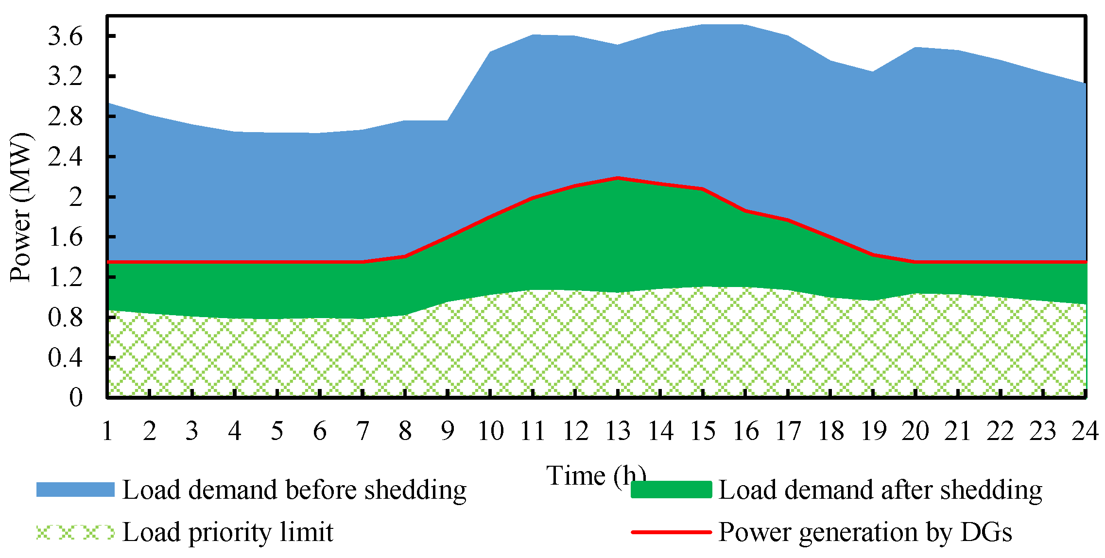
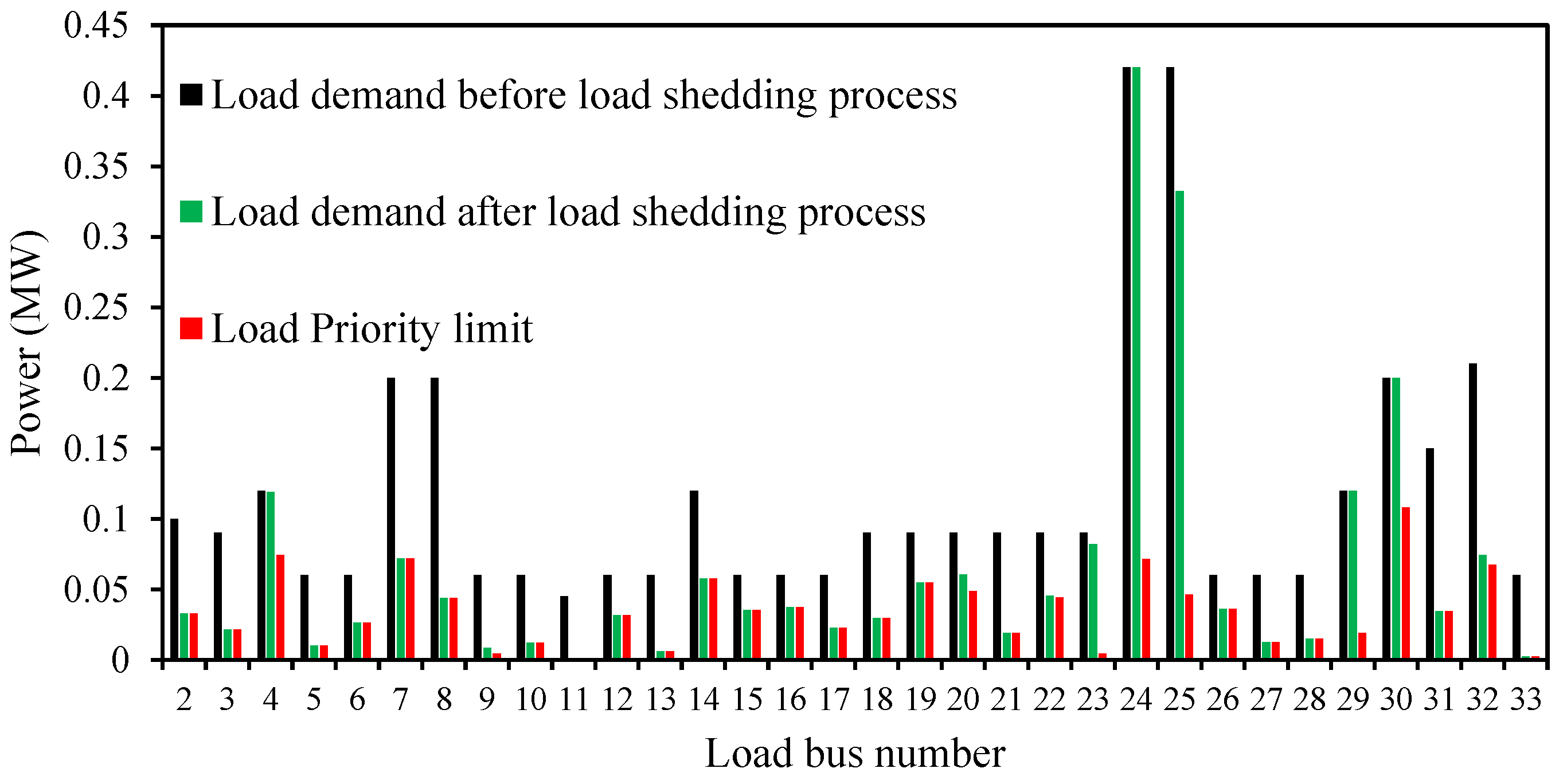
5. Simulation Results and Discussion of the Planning Load Shedding Scheme

In order to analyze the performance of the proposed method (FAPSO) against the PSO, FA, EP and GSA, all algorithms are implemented for load shedding. Table 3 shows the parameters for each algorithm.
For the values of population size and maximum iteration, there is no absolute way to determine them. However, from many simulations with different values, the current values for population size and maximum iteration was selected by try and error approach. Meanwhile, the parametric values used for the algorithms in the load shedding process was selected based on [44,45,46].
The simulation is used to demonstrate the performance of the FAPSO optimization. In this case, the proposed load shedding scheme is tested by considering the location and load priority limit. The limit, in this case, refers to the minimum percentage of load amount that should remain at a particular value after the load shedding process. The values are shown in Table 2.
A proposed load shedding scheme based on FAPSO is applied on a test system to maximize remaining load and improve voltage stability index. The fitness value is evaluated by using the Equation (2). The weightage set is varied in the range of 0 to 0.1 with a step size of 0.1. Based on the highest ηLAV value observed in Table 4, the weightage set of w1 = 0.8 and w2 = 0.2 is chosen as the best combination.
The values of the objective function were used to determine the light intensities of fireflies. The ranking of fireflies was utilized to determine and record the best firefly in the current generation. After many iterations, it can be noticed that the fireflies begin to report better fitness value. The fitness values can be computed by Equations (2)–(4). Meanwhile, the fireflies can be updated using Equation (20). The process is repeated until the stopping criteria are meet (number of iteration reaches to maximum number of iterations). FAPSO is controlled by four parameters: the randomization parameter (α), the attractiveness (β0), weighting factor c1 and the absorption coefficient (γ). These parameters need to be set within 0–1. Moreover, in order to realize the satisfactory implementation of the algorithm with less computational time, a suitable number of fireflies and maximum generation need to be determined. In this study, a set of experiments was carried out on the algorithm to do so. The tuned control parameters are tabulated in Table 3. The proposed algorithm was evaluated using the MATLAB (R2015a) environment on a 3.07 GHz CPU equipped with 8 GB RAM. The optimization was repeated 100 times, and the best final solution was selected as the final load remaining for each bus in the distribution networks.
In this case, the islanded system is formed when the main switch is opened as shown in Figure 4. Figure 7 shows the hourly power of the total load demand, total power generation from DGs, and grid for 24 h in grid connection mode. The figure demonstrates that the power imbalance between the load demand and power supply from DGs is huge, that is around 48–61% of the power generation curve to maximum daily load curve. When islanding is formed, load shedding needs to balance the generation and load demand to cater for the huge imbalance of power.
Since islanded could occur at any time, the proposed FAPSO for load shedding is tested every hour to analyze its overall performance in determining optimal load shedding. Figure 8 illustrates the amount of load and power from DGs as a result of load shedding if it occurs at any hour (within 24 h).
It can be seen that the amount of the remaining load after the load shedding process nearly matches the amount of power being supplied. This shows that that the proposed load-shedding technique based on the FAPSO optimization has the ability to identify the minimum amount of load to be curtailed without removing extra load from the network. It can also be observed that the proposed load-shedding technique based on FAPSO optimization realized the load priority limit requirement.
The load shedding result at time 15:00 is taken as an example to detail the performance of the proposed load shedding. At this time, the maximum load demand is 3.715 MW, as shown in Figure 7. However, the total power production at this hour is only 2.0764 MW, and the power deficit is around 44%. Thus, 44% of the load must be shed from the distribution network to prevent the system from collapse. After applying the proposed load shedding scheme, 1.6387 MW is removed, thus, the total remaining load is only 2.0763 MW, which closely matches the DGs power output.
The convergence characteristic for the proposed load shedding technique using the FAPSO optimization is shown in Figure 9 at time 15:00. It shows that the FAPSO converges and finds the solution after 157 iterations. Comparing the FAPSO results between the original load demands (black bar), remaining load after shedding (green bar), and load priority limit (red bar) for each bus are shown in Figure 10. From this comparison, it can be seen that load shedding fulfils the minimum load priority set in Table 2. There are also cases where the load at particular buses are not selected for shedding, examples being at buses 4, 24, 29 and 30.
Similarly, the load-shedding technique is performed and tested based on FA, PSO, EP and GSA algorithms. The EP is an optimization technique based on four main processes, which are initialization, mutation, competition and selection [47]. On the other hand, GSA algorithm has been developed for solving the real-value numerical optimization problems. The GSA algorithm has been inspired by the universal gravitational laws [34].
The purpose of this test is to validate the FAPSO algorithm in the proposed load-shedding technique and comparing its performance with all of FA, PSO, EP and GSA optimizations. For this study, the same time i.e., at time 15:00, is further analyzed for FA, PSO, EP and GSA optimizations. The voltage profile of the system before and when islanding occurs at time 15:00 is shown in Figure 11a. It can be clearly seen that islanding caused the overall voltage profile to decrease. However, when load shedding is applied using FAPSO, FA, PSO, EP and GSA optimizations at time 15:00, it can be seen that the voltage profiles after load shedding are all within the allowable limit, as per Figure 11b. It was also noted that minimum values of voltage profiles obtained using FA, PSO, EP and GSA optimizations are higher than the minimum value obtained using FAPSO. This took place due to the amount of loads that remaining in the distribution system using FAPSO optimization is larger than the others optimization techniques and the different amounts of load shed at particular buses. However, differences are regarded to be small.
After applying the load shedding technique based on both of FA, PSO, EP and GSA optimizations, the total remaining load suggested by FA, PSO, EP and GSA optimizations are 2.0643 MW 2.0649 MW, 1.61 MW and 2.0594 MW, respectively. These values are less than the amount determined by the FAPSO technique (2.0763 MW), which proves that the FAPSO is better than FA, PSO, EP and GSA algorithms in finding the optimal amount of remaining load, considering that the main objective of this study is to maximize the amount of load remaining without removing important loads from the system. The overall result of load shedding for all of the optimization methods is shown in Figure 12 for all buses. It can be seen that FA, PSO, EP and GSA shed more loads than FAPSO in the islanded system, where the percentage of total shed related to maximum acceptable shed value in the system are 63.16%, 63.14%, 80.55%, 63.35% and 62.70%, respectively. The results in Figure 12 prove that the FAPSO technique has the ability to remain loads without curtailment more than other techniques and this concurs with the objective of planning load shedding scheme.
Finally, Table 5 tabulates the summary of the comparison between the proposed load shedding based on the FAPSO optimization with each of FA, PSO, GSA, EP optimization. It can be seen from Table 5 that the load curtailment value done on the FAPSO optimization is the lowest value that keeps the voltage profile within the allowed limits.
The experimental results have been analyzed in 100 runs and the average fitness value, the best solution, and standard deviation of each of FA, PSO, GSA, EP and proposed algorithms are listed in Table 6. It can be seen that FAPSO outperforms the rest in terms of average fitness, the best solution, and standard deviation values. Therefore, these observations confirm that FAPSO shows better-searching performance with high precision. Table 6 also reveals the averaged running time (in seconds) of each of FA, PSO, GSA, EP and proposed algorithm on load shedding scheme in 100 runs. It can be noticed, the GSA is the faster algorithm to finish 300 iterations to find the final solution. However, it is of interest to note from Figure 9 that the proposed algorithm converges very fast as compared to FA, PSO, GSA and EP algorithms for load shedding scheme in the studied case. This is mean that the proposed algorithm can reach to the best solution in less time when compared with the other algorithms. Therefore, it confirms that FAPSO has efficient computational time at reaching the sub-optimal value. It is worth to mention, despite the computational time of GSA is faster than FAPSO, the important point in planning load shedding is achieving the best solution to apply the results to the system when needed. For that, the best solution is realized by FAPSO as shown in Table 6.

6. Test System for Proposed UFLS Scheme

The test system considered in this research is a part of the Malaysian distribution network shown in Figure 13. The test system consists of two mini-hydro DGs operated at a voltage level of 3.3 kV, each DG rated 2 MVA capacity (maximum power dispatch is 1.8 MW). The distribution network also consists of four PV generation units. As shown in Figure 13, four units of solar PV were connected with the network to work each rated 0.55 MWP. Two parallel units of solar PV plants were connected to 2 MVA step-up transformer (0.4 KV/11 kV); the total load demand of the distribution network is 6 MW, 2 Var. The mini-hydro units were connected to the distribution network using two step-up transformers (3.3 kV–11 kV). The distribution network with its DGs are modelled using the PSCAD/EMTDC software. The islanding operation is performed by opening the circuit breaker (BRKG) of Bus 2000. The modelling of the various components of the test system was explained in [47].
Generally, commercial and industrial loads are considered more important than its residential counterpart. For that, the residential loads from (Load 1–Load 10) can be randomly selected, as shown Table 7. The loads, with their priority rankings, are tabulated in Table 7.

7. Simulation Study of UFLS Scheme Using BFAPSO, BEP, BGSA, BPSO Techniques, and UFLS-FRPL

The simulation results included in this section are divided into three case studies:
  • The first case represents a comparative simulation study between, FA, PSO, GSA, EP, UFLS method proposed in [24], and FAPSO in terms of execution time.
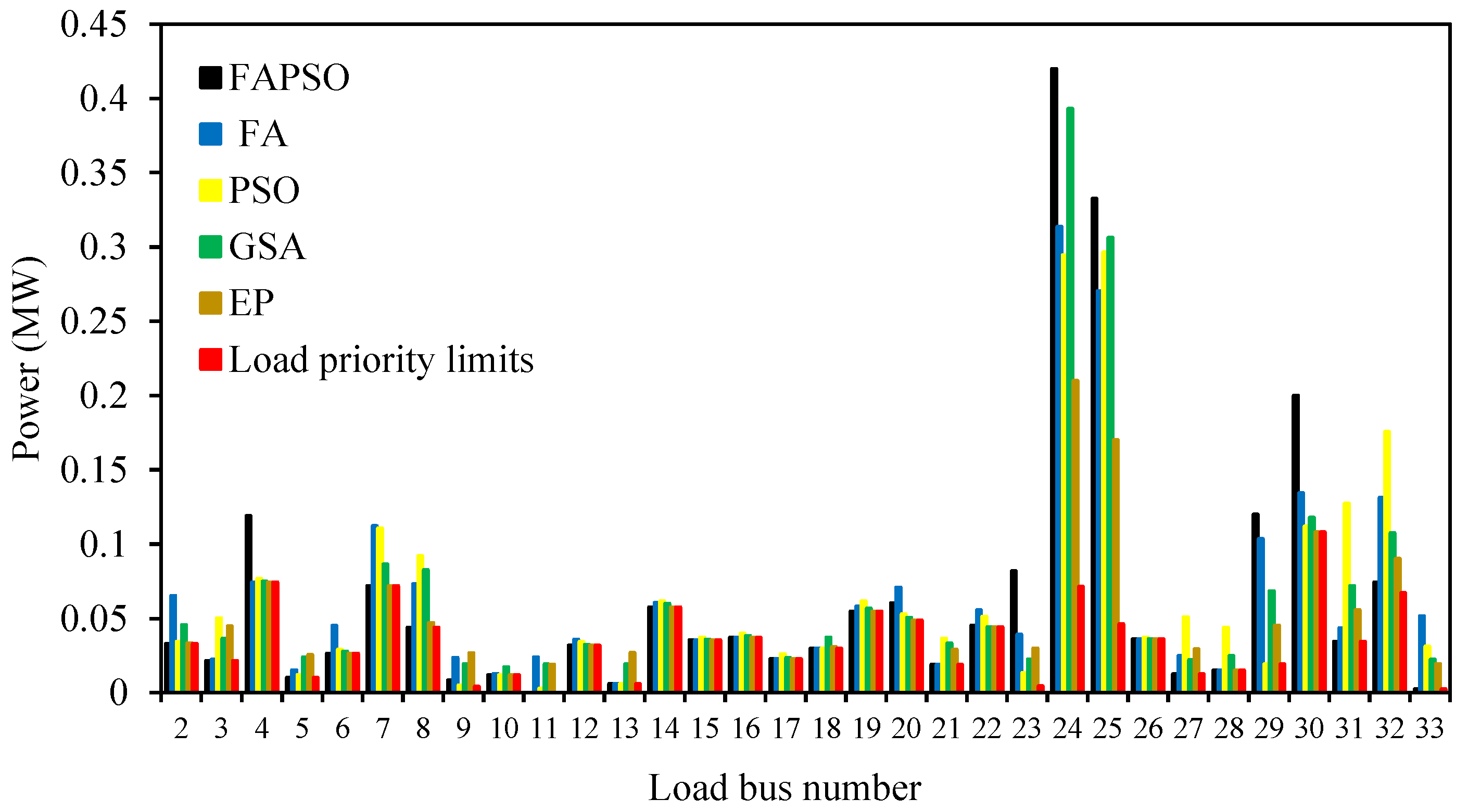
  • The second and third case study represent the simulation study of UFLS scheme for islanding case and adding extra load using FAPSO, FA, PSO, EP and GSA techniques, and UFLS method proposed in [24].

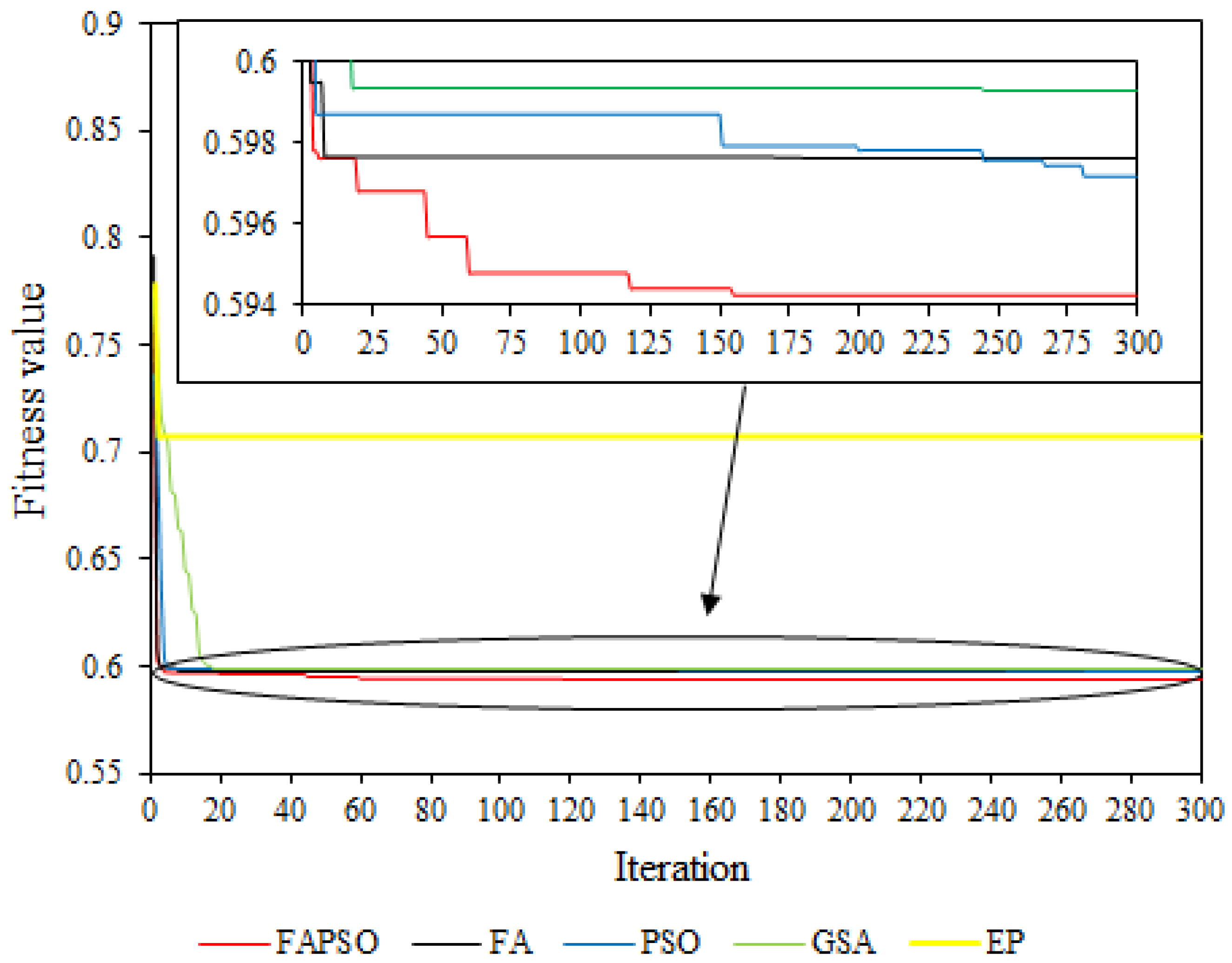
7.1. Comparison Between Different Metaheuristic Techniques in Term of Execution Time

The determination of optimal amount of load that should be shed is not a critical factor towards the success of load shedding technique, but also, the execution time that needed to implement the load shedding process is an important issue, too. The islanded distribution network with high penetration of DGs-based on power electronics suffers from rapid frequency changes due to reducing inertia response in power system. Accordingly, the load shedding controller will have a short time to make a decision. This study aims to compare the execution time of different metaheuristic methods and determine the best approach. The PC used in this work has a core i7 3.07 GHz processor and 8 GB RAM. Table 8 shows the execution times of six load shedding methods for six trials. In this comparison, the number of population is 20 and the maximum iteration number is 400. It is worth to mention, the iteration stops when the Equation (28) is reached, or if it reached its max iteration. It can be seen in Table 8 that the average of six execution times of FAPSO method is 17% of PSO, 14% of FA, 68% of GSA, 63% of EP and 20% of FRPLS technique proposed in [24]. Therefore, the FAPSO method is the best for the proposed UFLS technique.

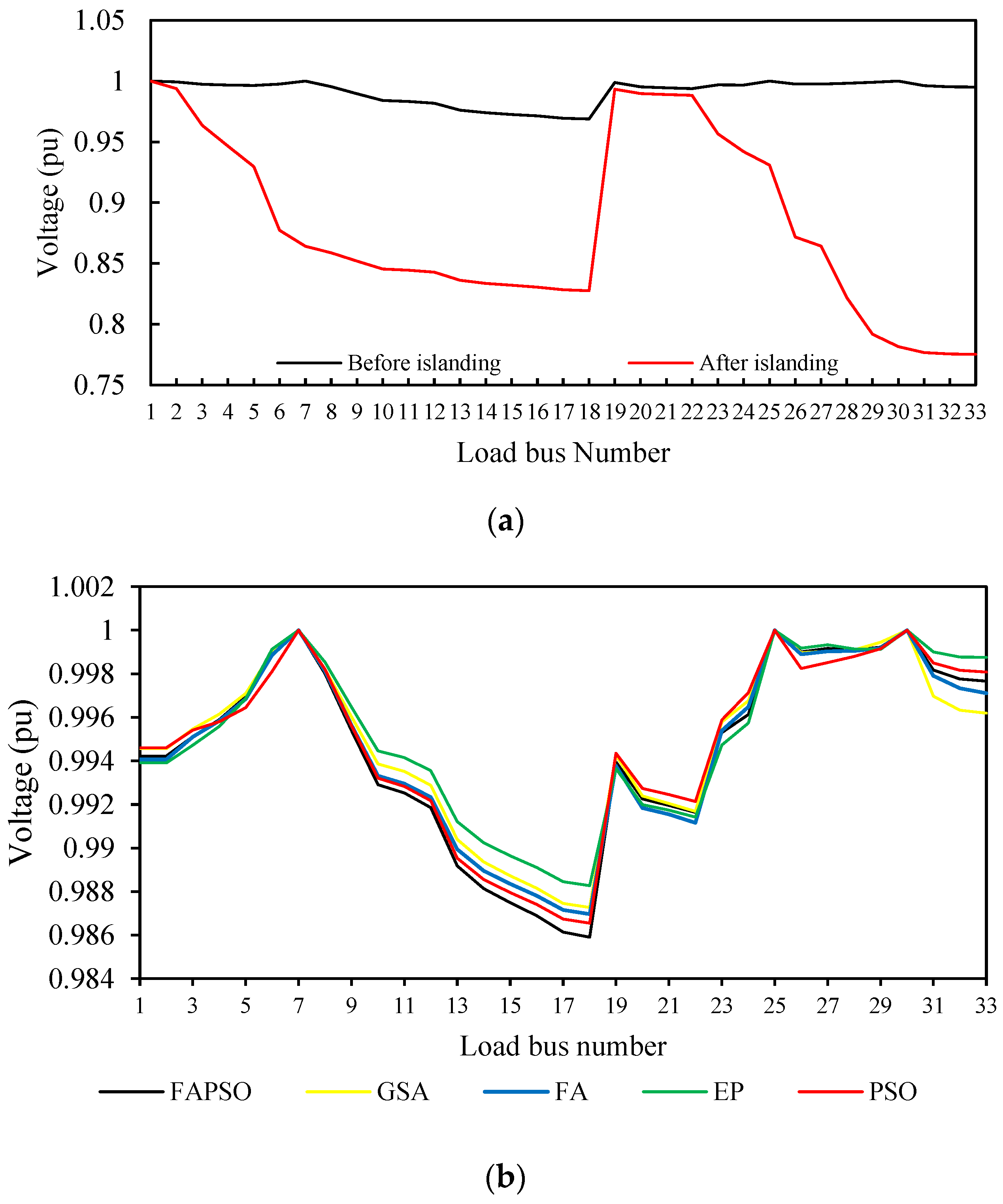
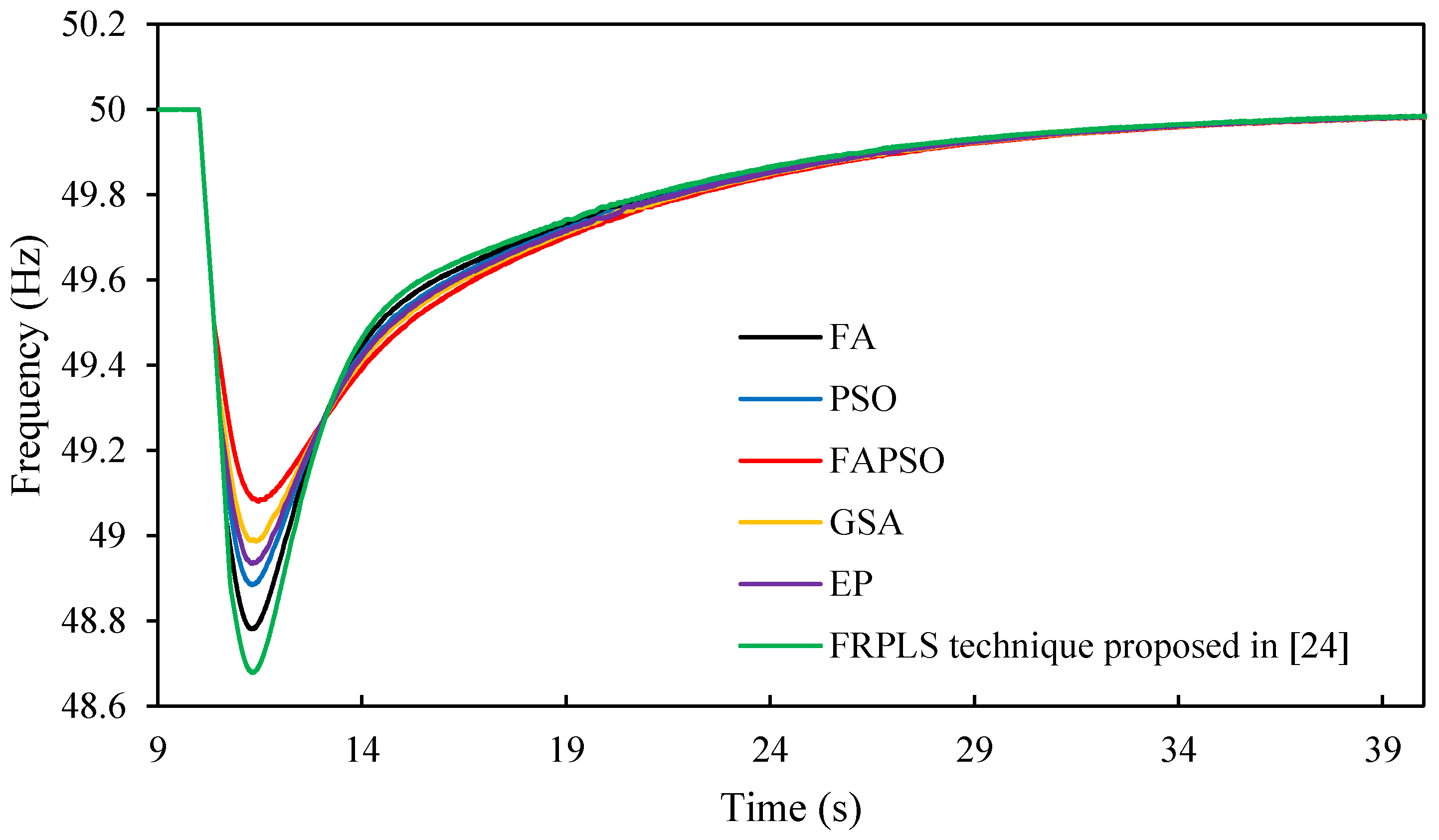
7.2. Intentional Islanding at 0.6 MW Imbalance Power

In this case, the intentional islanding happened at t = 10 s when the solar radiation value is 800 W/m2. After disconnecting the main grid which fed the distribution network by (0.6 MW), the frequency system immediately starts to decline. Due to this, the spinning reserve power of the mini-hydro generators is released by (0.18 MW). Because the spinning reserve power is inadequate to compensate for power deficit, a load shedding technique needs to be activated to rebalance the power between generation and demand and keep the system frequency within allowable limits. Table 9 shows that all optimization techniques will shed the same amount of power (0.427 MW). However, Figure 14 shows that the FAPSO technique successes to restore the system frequency to its’ nominal value with higher nadir frequency value. In fact, the large execution time of UFLS technique proposed in [24] is the main reason for less much of nadir frequency value.

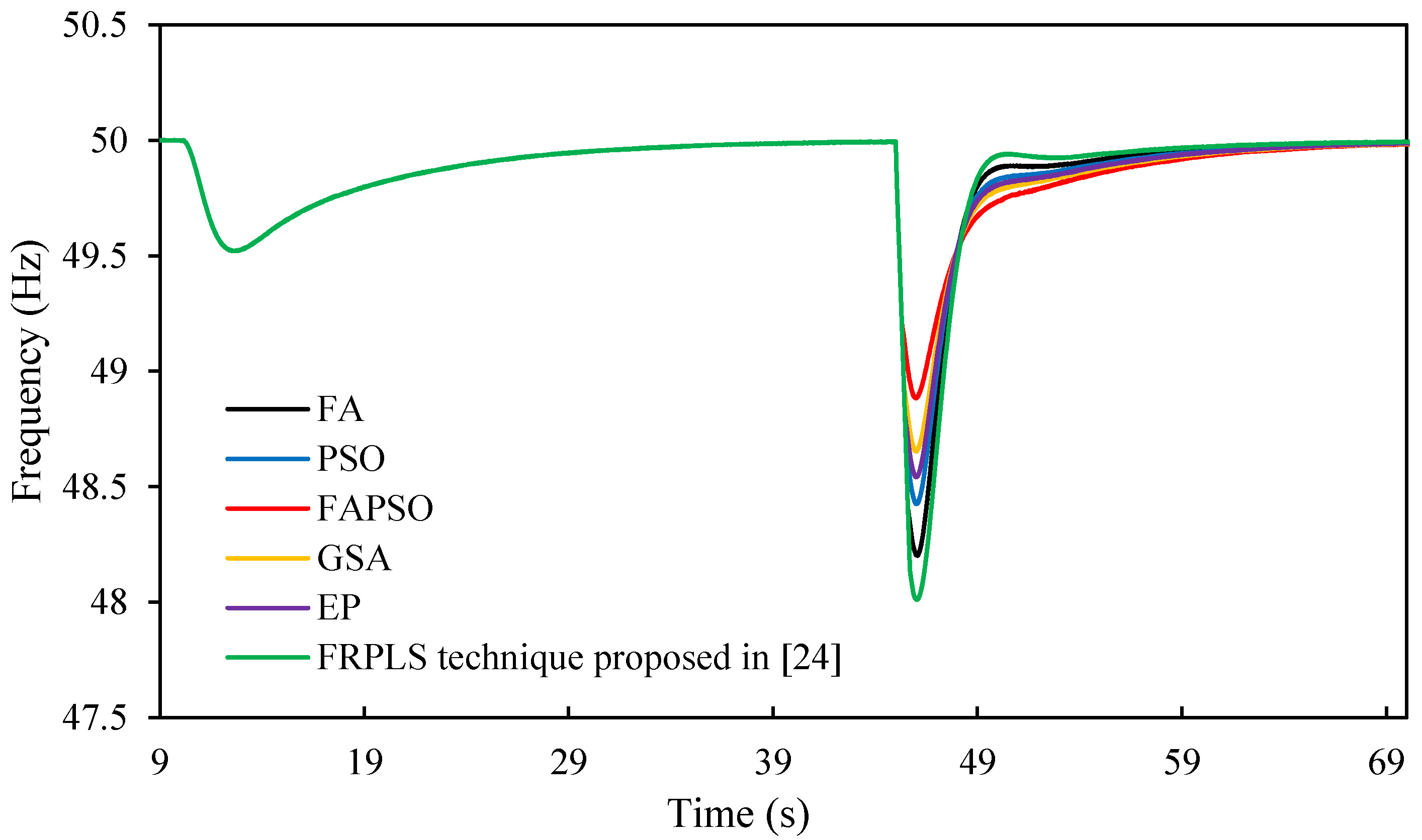
7.3. Load Increment of 0.9 MW

Immediately after islanding, the system frequency begins to decline in the response to an excess load of (0.113 MW). Accordingly, the mini-hydro generators use their spinning reserve (0.1 MW) to recover the unbalance of power. The UFLS controller will only be activated when the system frequency goes under 49.5 Hz. At 45 s, the total power demand will be 6.9 MW. Table 10 shows that all load shedding techniques will shed the same amount of power (0.897 MW). However, the frequency deviation for each technique is unequal due to the difference in execution time. The frequency responses of all UFLS controller are shown in Figure 15.

8. Conclusions

This work presents a hybrid FA-PSO based approach that aims to achieve an optimum load shedding scheme in an islanded distribution network. The proposed algorithm is suitable for planning load shedding schemes and UFLS schemes, because it utilizes the advantages of both the FA and PSO algorithms. The planning load shedding scheme based on FAPSO has been evaluated by solving a constrained optimization problem that aimed to simultaneously maximize the remaining loads of the islanded distribution network and keep the voltage profile within allowed limits in the islanding distribution network. The results of the proposed method in planning load shedding were compared with the FA, PSO, EP and GSA optimization techniques. This comparison showed that the proposed method performed well due to realizing the best maximum load remaining and improve voltage profile.
In practice, due to the growing penetration level of inverter-based DGs in distribution network, there is no total significant inertia and if a load-generation imbalance occurs, a fast frequency declination immediately takes place. To solve this problem, a quick UFLS scheme is needed to stop a system frequency declination and restore to its nominal value. Therefore, this paper also presented a new UFLS scheme that is suitable for islanding distribution networks. This UFLS scheme employs the application of hybrid FA-PSO algorithms to determine the optimal combination of loads that must to be removed from the distribution network with less execution time. The proposed UFLS scheme based on FAPSO was tested on the real distribution network. The results showed the proposed UFLS scheme is able to restore the systems’ frequency to its nominal value without overshooting. The proposed UFLS scheme based on FAPSO algorithm was also compared with UFLS scheme based on FA, PSO, EP and GSA techniques, and UFLS method proposed in [24] in the context of execution time. It can be concluded from the result that proposed UFLS scheme based on FAPSO algorithm can induce a high-speed response with the ability to disconnect optimal loads from islanded distribution network in a real application. In the future work, it can be developed a cooperative operation between the proposed UFLS scheme with inertia and frequency control schemes of RES-DGs and energy storage systems (ESSs) in the islanded distribution network. This development intends to realize a stable islanded distribution network and increase the local reliability from the viewpoint of loads/customers.

Author Contributions

Saad Mekhilef and Hazlie Mokhlis conceived and designed the experiments; Jafar Jallad, Javed Laghari and Ola Badran performed the experiments and analyzed the data; and Jafar Jallad wrote the paper.

Acknowledgments

This research is funded by University of Malaya under Postgraduate Research Grant (PPP): PG323-2016A.

Conflicts of Interest

The authors declare no conflict of interest.

References

  1. Eurostat: “Electricity Production and Supply Statistics”. Available online: http://epp.eurostat.ec.europa.eu/statistics_explained/index.php/Electricity_pproductio_and_supply_statiss (2012) (accessed on 20 September 2016).
  2. Hashim, H.; Ho, W.S. Renewable energy policies and initiatives for a sustainable energy future in Malaysia. Renew. Sustain. Energy Rev. 2011, 15, 4780–4787. [Google Scholar] [CrossRef]
  3. Fathi, M.; Bevrani, H. Statistical cooperative power dispatching in interconnected microgrids. IEEE Trans. Sustain. Energy 2013, 4, 586–593. [Google Scholar] [CrossRef]
  4. Cagnano, A.; Bugliari, A.C.; De Tuglie, E. A cooperative control for the reserve management of isolated microgrids. Appl. Energy 2018, 218, 256–265. [Google Scholar] [CrossRef]
  5. Hashiesh, F.; Mostafa, H.E.; Khatib, A.-R.; Helal, I.; Mansour, M.M. An intelligent wide area synchrophasor based system for predicting and mitigating transient instabilities. IEEE Trans. Smart Grid 2012, 3, 645–652. [Google Scholar] [CrossRef]
  6. Xue, Y.; Xiao, S. Generalized congestion of power systems: Insights from the massive blackouts in India. J. Mod. Power Syst. Clean Energy 2013, 1, 91–100. [Google Scholar] [CrossRef]
  7. Hsu, C.-T.; Chuang, H.-J.; Chen, C.-S. Adaptive load shedding for an industrial petroleum cogeneration system. Expert Syst. Appl. 2011, 38, 13967–13974. [Google Scholar] [CrossRef]
  8. Hsu, C.-T.; Kang, M.-S.; Chen, C.-S. Design of adaptive load shedding by artificial neural networks. IEE Proc.-Gener. Transm. Distrib. 2005, 152, 415–421. [Google Scholar] [CrossRef]
  9. Hooshmand, R.; Moazzami, M. Optimal design of adaptive under frequency load shedding using artificial neural networks in isolated power system. Int. J. Electr. Power 2012, 42, 220–228. [Google Scholar] [CrossRef]
  10. Sallam, A.; Khafaga, A. Fuzzy expert system using load shedding for voltage instability control. In Proceedings of the IEEE Conference on Power Engineering Large Engineering Systems, LESCOPE 02, Halifax, NS, Canada, 26–28 June 2002; pp. 125–132. [Google Scholar]
  11. Mokhlis, H.; Laghari, J.; Bakar, A.; Karimi, M. A fuzzy based under-frequency load shedding scheme for islanded distribution network connected with DG. Int. Rev. Electr. Eng. 2012, 7, 4992–5000. [Google Scholar]
  12. Ketabi, A.; Fini, M.H. Adaptive underfrequency load shedding using particle swarm optimization algorithm. J. Appl. Res. Technol. 2017, 15, 54–60. [Google Scholar] [CrossRef]
  13. Sanaye-Pasand, M.; Davarpanah, M. A new adaptive multidimensioanal load shedding scheme using genetic algorithm. In Proceedings of the Canadian Conference on IEEE Electrical and Computer Engineering, Saskatoon, SK, Canada, 1–4 May 2005; pp. 1974–1977. [Google Scholar]
  14. Chen, C.-R.; Tsai, W.-T.; Chen, H.-Y.; Lee, C.-Y.; Chen, C.-J.; Lan, H.-W. Optimal load shedding planning with genetic algorithm. In Proceedings of the Conference on IEEE Industry Applications Society Annual Meeting (IAS), Orlando, FL, USA, 9–13 October 2011; pp. 1–6. [Google Scholar]
  15. Amraee, T.; Mozafari, B.; Ranjbar, A. An improved model for optimal under voltage load shedding: Particle swarm approach. In Proceedings of the Conference on IEEE Power India, New Delhi, India, 10–12 April 2006. [Google Scholar]
  16. Sadati, N.; Amraee, T.; Ranjbar, A. A global particle swarm-based-simulated annealing optimization technique for under-voltage load shedding problem. Appl. Soft Comput. 2009, 9, 652–657. [Google Scholar] [CrossRef]
  17. Pal, S.K.; Rai, C.; Singh, A.P. Comparative study of firefly algorithm and particle swarm optimization for noisy non-linear optimization problems. IJISA 2012, 4, 50–57. [Google Scholar] [CrossRef]
  18. Niknam, T.; Narimani, M.R.; Jabbari, M. Dynamic optimal power flow using hybrid particle swarm optimization and simulated annealing. Int. Trans. Electr. Energy 2013, 23, 975–1001. [Google Scholar] [CrossRef]
  19. Lu, Y.; Kao, W.-S.; Chen, Y.-T. Study of applying load shedding scheme with dynamic D-factor values of various dynamic load models to Taiwan power system. IEEE Trans. Power Syst. 2005, 20, 1976–1984. [Google Scholar] [CrossRef]
  20. Kundur, P.; Balu, N.J.; Lauby, M.G. Power System Stability and Control; McGraw-Hill: New York, NY, USA, 1994; Volume 7. [Google Scholar]
  21. Maliszewski, R.; Dunlop, R.; Wilson, G. Frequency actuated load shedding and restoration part I-Philosophy. IEEE Trans. Power App. Syst. 1971, PAS-90, 1452–1459. [Google Scholar] [CrossRef]
  22. Seethalekshmi, K.; Singh, S.N.; Srivastava, S.C. A synchrophasor assisted frequency and voltage stability based load shedding scheme for self-healing of power system. IEEE Trans. Smart Grid 2011, 2, 221–230. [Google Scholar] [CrossRef]
  23. Andersson, D.; Elmersson, P.; Juntti, A.; Gajic, Z.; Karlsson, D.; Fabiano, L. Intelligent load shedding to counteract power system instability. In Proceedings of the IEEE/PES Transmission and Distribution Conference and Exposition: Latin America, Sao Paulo, Brazil, 8–11 November 2004; pp. 570–574. [Google Scholar]
  24. Laghari, J.; Mokhlis, H.; Karimi, M.; Bakar, A.H.A.; Mohamad, H. A new under-frequency load shedding technique based on combination of fixed and random priority of loads for smart grid applications. IEEE Trans. Power Syst. 2015, 30, 2507–2515. [Google Scholar] [CrossRef]
  25. Rudez, U.; Mihalic, R. Monitoring the first frequency derivative to improve adaptive underfrequency load-shedding schemes. IEEE Trans. Power Syst. 2011, 26, 839–846. [Google Scholar] [CrossRef]
  26. Anderson, P.; Mirheydar, M. An adaptive method for setting underfrequency load shedding relays. IEEE Trans. Power Syst. 1992, 7, 647–655. [Google Scholar] [CrossRef]
  27. Jung, J.; Liu, C.-C.; Tanimoto, S.L.; Vittal, V. Adaptation in load shedding under vulnerable operating conditions. IEEE Trans. Power Syst. 2002, 17, 1199–1205. [Google Scholar] [CrossRef]
  28. Laghari, J.; Mokhlis, H.; Bakar, A.H.A.; Karimi, M.; Shahriari, A. An intelligent under frequency load shedding scheme for islanded distribution network. In Proceedings of the Power Engineering and Optimization Conference (PEDCO), Melaka, Malaysia, 6–7 June 2012; pp. 40–45. [Google Scholar]
  29. Hong, Y.-Y.; Wei, S.-F. Multiobjective underfrequency load shedding in an autonomous system using hierarchical genetic algorithms. IEEE Trans. Power Del. 2010, 25, 1355–1362. [Google Scholar] [CrossRef]
  30. Mahat, P.; Chen, Z.; Bak-Jensen, B. Underfrequency load shedding for an islanded distribution system with distributed generators. IEEE Trans. Power Del. 2010, 25, 911–918. [Google Scholar] [CrossRef]
  31. Zin, A.M.; Hafiz, H.M.; Wong, W. Static and dynamic under-frequency load shedding. In Proceedings of the International IEEE Conference on Power System Technology, Singapore, Singapore, 21–24 November 2004; pp. 941–945. [Google Scholar]
  32. Chakravorty, M.; Das, D. Voltage stability analysis of radial distribution networks. Int. J. Electr. Power 2001, 23, 129–135. [Google Scholar] [CrossRef]
  33. Das, D.; Kothari, D.; Kalam, A. Simple and efficient method for load flow solution of radial distribution networks. Int. J. Electr. Power 1995, 17, 335–346. [Google Scholar] [CrossRef]
  34. Garg, J.; Swami, P. Calculating voltage instability using index analysis in radial distribution system. Int. J. Mod. Eng. Res. 2014, 4, 15–26. [Google Scholar]
  35. Aziz, N.I.A.; Sulaiman, S.I.; Musirin, I.; Shaari, S. Assessment of evolutionary programming models for single-objective optimization. In Proceedings of the 7th International IEEE Power Engineering and Optimization Conference (PEOCO), Langkawi, Malaysia, 3–4 June 2013; pp. 304–308. [Google Scholar]
  36. Rahim, S.A.; Rahman, T.A.; Musirin, I.; Azmi, S.; Mohammed, M.; Hussain, M.; Faridun, M. Comparing the network performance between the installation of DG and compensating capacitor using EP. Int. J. Power Energy Artif. Intell. 2008, 1, 14–21. [Google Scholar]
  37. Rashedi, E.; Nezamabadi-Pour, H.; Saryazdi, S. GSA: A gravitational search algorithm. Inf. Sci. 2009, 179, 2232–2248. [Google Scholar] [CrossRef]
  38. Yang, X.-S. Nature-Inspired Metaheuristic Algorithms; Luniver Press: Bristol, UK, 2010. [Google Scholar]
  39. Gandomi, A.H.; Yang, X.-S.; Alavi, A.H. Mixed variable structural optimization using firefly algorithm. Comput. Struct. 2011, 89, 2325–2336. [Google Scholar] [CrossRef]
  40. Eberhart, R.; Kennedy, J. A new optimizer using particle swarm theory. In Proceedings of the IEEE Proceedings of the Sixth International Symposium on Micro Machine and Human Science (MHS’95), Nagoya, Japan, 4–6 October 1995; pp. 39–43. [Google Scholar]
  41. Liu, H.; Chen, Z. Contribution of VSC-HVDC to frequency regulation of power systems with offshore wind generation. IEEE Trans. Energy Convers. 2015, 30, 918–926. [Google Scholar] [CrossRef]
  42. Aponte, E.E.; Nelson, J.K. Time optimal load shedding for distributed power systems. IEEE Trans. Power Syst. 2006, 21, 269–277. [Google Scholar] [CrossRef]
  43. Baran, M.E.; Wu, F.F. Network reconfiguration in distribution systems for loss reduction and load balancing. IEEE Trans. Power Del. 1989, 4, 1401–1407. [Google Scholar] [CrossRef]
  44. Shi, Y.; Eberhart, R.C. Empirical study of particle swarm optimization. In Proceedings of the IEEE Congress on Evolutionary Computation (CEC 99), Washington, DC, USA, 6–9 July 1999; pp. 1945–1950. [Google Scholar]
  45. Badran, O.; Mokhlis, H.; Mekhilef, S.; Dahalan, W. Multi-Objective Network Reconfiguration with Optimal DG Output Using Meta-Heuristic Search Algorithms. Arab. J. Sci. Eng. 2017, 1–14. [Google Scholar] [CrossRef]
  46. Lu, P.; Ye, L.; Sun, B.; Zhang, C.; Zhao, Y.; Zhu, T. A New Hybrid Prediction Method of Ultra-Short-Term Wind Power Forecasting Based on EEMD-PE and LSSVM Optimized by the GSA. Energies 2018, 11, 697. [Google Scholar] [CrossRef]
  47. Dreidy, M.; Mokhlis, H.; Mekhilef, S. Application of Meta-Heuristic Techniques for Optimal Load Shedding in Islanded Distribution Network with High Penetration of Solar PV Generation. Energies 2017, 10, 150. [Google Scholar] [CrossRef]
Figure 1. Two bus power system model.
Energies 11 01134 g001
Figure 2. Flowchart of proposed algorithm (FAPSO).
Energies 11 01134 g002
Figure 3. Flowchart of proposed planning load shedding scheme.
Energies 11 01134 g003
Figure 4. Test system.
Energies 11 01134 g004
Figure 5. Hourly PV power production by DG3.
Energies 11 01134 g005
Figure 6. Hourly load profile for individual loads.
Energies 11 01134 g006
Figure 7. Daily load curve and power supply by grid and DGs.
Energies 11 01134 g007
Figure 8. Load demand before/after applying the proposed load-shedding technique by hybrid FAPSO.
Energies 11 01134 g008
Figure 9. Convergence characteristic for FAPSO, FA PSO, GSA and EP optimizations at time 15:00.
Energies 11 01134 g009
Figure 10. Loads demand at each bus after performing the proposed load-shedding technique at time 15:00 hour for island with their load priority limits.
Energies 11 01134 g010
Figure 11. Voltage profile for the simulation: (a) Voltage profile before and after islanding at time 15:00 without load shedding; (b) Voltage profile after applying techniques FAPSO, FA, PSO, EP and GSA optimizations at time 15:00.
Energies 11 01134 g011
Figure 12. Load buses demand after implementing the load shedding process based on FAPSO, FA, PSO, EP and GSA optimizations at time 15:00 for island case 1.
Energies 11 01134 g012
Figure 13. The distribution network for validation of proposed Under Frequency Load Shedding (UFLS) technique.
Energies 11 01134 g013
Figure 14. Frequency response of intentional islanding at 0.6 MW imbalance power.
Energies 11 01134 g014
Figure 15. Frequency response for 0.9 MW load increment.
Energies 11 01134 g015
Table 1. Maximum active power produced by Distributed Generators (DGs).
DG NumberBus NumberType of DGMaximum Output Power (MW)Power Factor
17Mini-Hydro0.850.8
225Mini-Hydro0.50.8
330PV0.8371
Table 2. The minimum percentage of load priority limit for each bus.
Bus No.Percentage (%)Bus No.Percentage (%)
2331961
3242054
4622121
5172249
644235
7362417
8222511
972660
10202721
1102825
12532916
13103054
14483123
15593232
1662334
1738--
1833--
Table 3. Particle Swarm Optimization (PSO), Firefly Algorithm (FA), Firefly Algorithm—Particle Swarm Optimization (FAPSO), Evolutionary Programming (EP) and Gravitational Search Algorithm (GSA) Parameters Setting.
ParameterPSOFAFAPSOEPGSA
Population size (N)5050505050
Maximum iteration (n)300300300300300
Parameters values that used for algorithmwmax = 0.9
wmin = 0.4
c1 = 2
c2 = 2
β0 = 0.2
γ = 1
α = 0.8
β0 = 0.2
γ = 1
α = 0.8
c1 = 2
-G0 = 100
α = 10
Table 4. Weightage set and corresponding performance index based on Least Average Value (LAV) by applying proposed load shedding with consideration priority limit at time 15:00.
No.w1w2Remaining Load (MW)Minimum Value of SIηLAV
1101.9748020.95147534.86
20.90.12.039360.95020978.63
30.80.22.076370.9568464178.4
40.70.32.0348780.95247279.10
50.60.41.8907520.94188617.49
60.50.52.0685090.944912119.49
70.40.62.0313230.94020349.77
80.30.72.033760.9533880.36
90.20.81.9872420.9504838.57
100.10.91.7840580.95730412.22
11011.1149390.9573042.32
Table 5. Summary for comparison in performance of FAPSO, FA, PSO, GSA and EP in load shedding technique.
AlgorithmsApplying Optimal Load Shedding with Consideration Priority Limit at Time 15:00
FitnessMinimum Voltage of Load BusLoad Curtailment %
PSO0.597190.9865444.43
FA0.597590.9869644.46
FAPSO0.594240.9859044.11
GSA0.599290.98727144.56
EP0.707260.98827156.66
Table 6. Comparison of mean fitness value, best solution, standard deviation and average computational time for 100 runs on load shedding scheme.
Population Size/Max IterationIndicesAlgorithms
EPGSAFAPSOFAPSO
50/300Average fitness0.779240.599880.599390.599040.59468
Best solution0.707260.599290.597600.597190.59419
Standard deviation0.0314760.000395880.000503780.00088660.00032375
Average computational time (seconds)661.21330.01760.58655.7708.11
Table 7. Load data and their priority.
Load RankedBus No.P (MW)Load Priority
Load 110500.044Random
Load 210130.069Random
Load 31047,10260.15Random
Load 410120.314Random
Load 511510.5Random
Load 610290.55Random
Load 71010,10390.583Random
Load 810750.645Random
Load 91018–1020, 10460.7Random
Load 1011440.119Random
Table 8. The execution time for different load shedding scenarios.
Trial NumberExecution Time (Second)
FAPSOFAPSOGSAEPFRPLS Technique Proposed in [24]
10.7230.6090.1220.130.1550.5
20.7120.6070.060.1430.1530.5
30.7030.6050.110.1090.1530.5
40.7870.6460.1450.250.1520.5
50.6570.6570.050.150.1620.5
60.7410.6260.1010.090.150.5
Average0.72050.6250.0980.1450.1540.5
Table 9. The UFLS parameters of intentional islanding at 0.6 MW imbalance power.
ParameterFAPSOFAPSOGSAEPUFLS Technique Proposed in [24]
ΔP (MW)0.60.60.60.60.60.6
Reserve (MW)0.180.180.180.180.180.18
Total Load Shed Power (MW)0.4270.4270.4270.4270.4270.427
Shedding loadsLoads
1,2,4
Loads
1,2,4
Loads
1,2,4
Loads
1,2,4
Loads
1,2,4
Loads
1,2,4
Nadir Frequency (Hz)48.248.4248.8848.6548.5448.01
Table 10. The UFLS parameters for load increment of 0.9 MW after islanding.
ParameterFAPSOFAPSOGSAEPFRPLS Technique Proposed in [24]
ΔP (MW)0.90.90.90.90.90.9
Reserve (MW)000000
Total Load Shed Power (MW)0.8970.8970.8970.8970.8970.897
Shedding loadsLoads 4,7Loads 4,7Loads 4,7Loads 4,7Loads 4,7Loads 4,7
Nadir Frequency (Hz)48.248.4248.8848.6548.5448.01

