Abstract
Nowadays, problems facing Distribution System Operators (DSOs) due to demand increase and the wide penetration of renewable energy are usually solved by means of grid reinforcement. However, the smart grid paradigm enables the deployment of demand flexibility for congestion management in distribution grids. This could substitute, or at least postpone, these needed investments. A key role in this scheme is the aggregator, who can act as a “flexibility provider” collecting the available flexibility from the consumers. Under this paradigm, this paper proposes a flexibility market led by the DSO and aimed at solving distribution grid congestions. The proposal also includes a flexibility market clearing algorithm, which is easy to implement, has low computational requirements and considers the energy rebound effect. The proposed design has the advantage of excluding the DSO’s need for trading in energy markets. Also, the solution algorithm proposed is fully compatible with already existing grid analysis tools. The proposed electricity market is tested with two case studies from a real Spanish distribution network, where the proposed clearing algorithm is used, and finally, results are presented and discussed.
1. Introduction
The deployment of new technologies to manage the grid operational levels, starting from the generation and down to the demand level, is set to create a reliable, efficient and economic power system. This is one of the main benefits of the current evolution of conventional electric grids into smarter and more flexible ones. However, the wide penetration of low carbon technologies, accompanied with the increase of electricity demand, has imposed many challenges on distribution networks. Consequently, various market players and policy makers have encouraged the idea of flexible resources as a way of coping with such challenges. New technologies such as intelligent smart meters, autonomous load controllers and advanced information and communication automations, are capable of providing sustainable minute-by-minute information to efficiently deploy demand response (DR) programs [1,2].
DR are programs established to encourage end-user customers in adjusting their electric usage, in response to changes in electricity prices over time, or incentive payments [3]. DR programs help reducing electricity consumption at hours of high demand or uphold the reliability of electrical systems when their security is jeopardized [4,5]. This paper focuses on demand side flexibility (DSF), which is one of main types of incentive-based DR programs [6,7,8]. DSF encourages customers to actively participate in electricity markets by submitting increasing or decreasing capacity volumes [9,10,11]. Moreover, DSF can be used as a portfolio optimization source for market players who need to meet their energy requirements. Besides, it can provide balancing and constraint management services for system operators such as transmission and distribution system operators (TSOs) and (DSOs), to maintain system reliability and security [12]. However, the deployment of DSF faces many challenges that vastly impacts its value [13]. The absence of appropriate market mechanisms in current market structures is one of the main causes of delaying its full potential [14]. Other considerations must be faced in insular systems, where security issues are even more pressing than in large continental grids, as remarked in [15], and a risk analysis is advisable in order to deal with them for the daily operational planning. Besides, in insular systems, the DSO can dispatch generation and storage units.
The objective of this paper is optimizing the usage of DSF in a day-ahead timeframe at the distribution level to assist the DSO in mitigating network congestions. There has been vast literature addressing this issue, for example, a day-ahead planning framework for flexible demand bidding strategies is introduced in [16]. The objective of the proposed model is to maximize the profit for the flexibility providers by forecasting the aggregated load demand of customers and consecutively building flexibility offers. Similarly, another short-term planning models for optimal flexibility bidding are introduced in [17,18]. These studies focus on the effect of price elasticity on short-term planning in the framework of day-ahead markets. A decision making problem for optimal flexible energy resources scheduling to meet the DSO requests was suggested in [19]. The paper proposes a new type of aggregator called smart energy provider (SESP) to handle all flexible energy sources. Moreover, it presents a local electricity market for flexibility trading. Optimization models focusing on maximizing the potential of DSF and the financial benefits for both, customers and system operators, are addressed in [20,21,22]. Such studies have concluded that the efficient usage of DSF at the hours of grid contingencies can alleviate such congestions, thus increasing the reliability of the grid operation. Furthermore, DSF can help in deferring the need of grid reinforcements in many cases [23].
While the aforementioned studies are significant contributions, they mainly focus on the bidding processes, bidding strategies and effects of price elasticity. However, less attention has been given to the effects of demand flexibility in mitigating network congestions. In addition, two mutually important key factors were absent in previous works. First factor has to do with grid power flow constraints. In general, the optimal operation of transmission and distribution networks is controlled by close monitoring of the power flow within the grid and the voltage levels at every node. Modelling the grid constraints can be problematic due to its complexity. However, considering them is essential to realistically model the impact of demand flexibility activations at the distribution level. Secondly, in most cases when customers are asked to provide demand flexibility, their loads are shifted from one point in time to another. This shift can alleviate one congestion and create another one by moving the peak from high priced hours to low priced hours. This effect is regarded in literature as the rebound effect or payback effect [24]. Such event is crucial to the flexibility beneficiaries as they must consider the repercussions of activating flexibility services on their day-ahead operation.
The work presented here aims to build on what was carried out in [25,26,27] and further advance towards presenting a realistic framework for demand flexibility management. The proposed framework considers two types of demand flexibility, load increase and decrease volumes that can be a valuable tool to the DSO in the congestion management process. In addition, the paper exploits the demand flexibility that can be obtained from the industrial and residential sectors. Two real distribution network feeders in Spain are used as case studies to show the advantages that demand flexibility types can offer in the process of congestion solution, while minimizing the cost of flexibility procurement for the DSO. The main contributions of this paper are:
- Proposing a simple but realistic model for a flexibility market operating at the distribution level. This market serves as a platform for flexibility transactions and it facilitates the trading between flexibility beneficiaries and providers. The flexibility market is operated by the DSO and it takes place after the day-ahead wholesale market. The proposed market structure does not require complex changes in regulations and it avoids the DSO’s need to participate in energy trading.
- Formulating and solving an optimization problem that models the total cost incurred by the DSO when activating the flexibility services. The method is easy to implement and can be integrated with already existing Optimal Power Flow (OPF) solver tools. The grid power flow constraints and the rebound conditions are considered and modeled. Therefore, the DSO always performs a technical validation of the demand flexibility solution, avoiding unforeseen problems that can arise from the rebound effect.
It must be remarked that the proposed flexibility market mechanism does not deal with security issues that must be solved using a different method, even without making use of market solutions. A risk analysis should be performed in order to meet the security requirements of a distribution system when demand response is considered. This analysis, however, is out of the scope of the paper.
The organization of this paper can be described as follows. In Section 2, an overview about demand flexibility is given along with the stakeholders involved in its paradigm. In Section 3, the proposed flexibility market is introduced and explained. Section 4 discusses the problem formulation regarding optimizing the cost of purchasing DSF. Moreover, Section 5 carries out a detailed two-case study to highlight the merits of DSF in efficiently managing grid congestions. Finally, Section 6 concludes the paper.
2. Demand Flexibility Overview & Stakeholders
Flexibility can be defined as the ability of adjusting generation and/or consumption profiles in response to external market signals. It can be utilized to provide energy balancing services for TSOs and balance responsible parties (BRPs), power quality control or, as proposed here, congestion management [11]. Demand flexibility has been used for many years at the transmission level in some countries, and expanding it to the distribution level is becoming feasible and convenient. However, a number of challenges must be addressed to allow its implementation [28]. In this section, the different kinds of flexibility used, the stakeholders involved and the roles that they can play in flexibility markets are described.
2.1. Demand Flexibility Types
The shape, quantity and direction of available flexibility may vary depending on the type of the customer. Such features determine the way flexibility is integrated into electricity markets [29]. Here, demand flexibility is addressed from the DSO’s perspective. Since the flexibility offered by the demand side can take the form of either increasing or decreasing the load, two kinds of flexibility are defined, named up-regulation (UREG) and down-regulation (DREG) flexibility. Customers offering UREG flexibility provide load reduction volumes, while customers offering DREG flexibility provide load increase volumes. In a market-oriented approach for flexibility management, such as the one considered here, these volumes can be translated into up-regulation bids (URB) and down-regulation bids (DRB) respectively and can be offered for sale to other market participants.
Demand flexibility consists of increasing or decreasing the load at one hour, which then may require shifting that amount to another hour. This shifting of energy may produce further problems in the grid, for instance, if the reduced energy due to UREG flexibility is recovered by the customer at a load peak hour, producing further congestion. This can be referred to as the energy rebound effect [30]. Thus, it is essential for the DSO to consider the rebound effect properly when managing demand flexibility. Moreover, the conditions under which the rebound effect takes place should be agreed upon between the flexibility supplier and the DSO. The rebound conditions considered here are the rebound hour and the rebound power. The rebound hour is the hour at which the regulation power is shifted to, while the rebound power is the share of regulation power (UREG or DREG) that must be recovered to the customer. The rebound conditions are dependent on the type of customers and the nature of the load providing the flexibility. For example, the rebound power can either be equal to the activated flexibility, or just a percentage of it. For the rebound hour, customers have the possibility of deciding the most convenient hour to have the rebound power. Therefore, rebound hour can either be a specific hour, or any hour during a time interval of the day or it can be unrestricted. Considering the rebound effect of demand flexibility is crucial for the DSO to avoid possible subsequent problems in the network. However, it adds further complexities to the task of the DSO. In very large networks with thousands of customers and possibly hundreds of aggregated flexibility bids, choosing the optimal bid may require sophisticated mathematical methods and computing power.
In order to differentiate between the rebound power of both UREG and DREG flexibilities, two different names will be assigned to each one of them. Since UREG requires supplying back the regulation power at the rebound hour, the rebound effect will be referred to as the payback effect (PB), with payback power at the payback hour [31]. On the other hand, as the DREG requires a decrease of the load at the rebound hour, it will be referred to as the rebate effect (REB), with rebate power at the rebate hour. As already mentioned, in certain cases the rebound effect may create new network congestions. Such cases may occur if the PB creates unexpected new peaks, or when the REB decreases the load leading to overvoltages. Table 1 summarizes the types of DSF with their corresponding type of rebound effect. It should be noted that, while previous work has discussed the payback effect from the perspective of UREG flexibility [24], there are no current studies that address the rebound effect in case of DREG flexibility, up to the knowledge of the authors.

Table 1.
Summary of DSF types.
The involvement of the main stakeholders expected to be connected to the management of demand flexibility is summarized in the following subsections.
2.2. Distribution System Operators (DSOs)
Demand flexibility allows the DSO to manage grid congestions by avoiding demand peaks. This can possibly lead to deferring the need for network reinforcements [32], decreasing the total capital and operation expenditures of distribution networks [33]. In addition, demand flexibility provides more resources to manage the requirements of the increasingly high penetration of DERs based on RES. One of the key factors to ensure the success of flexibility is having the necessary coordination between the DSO and TSO. Such coordination is essential to avoid needles flexibility requirements which can lead to further grid problems [34].
Here, demand flexibility is modeled and centered on tackling the issue of congestion management at the distribution level. While there is a major potential for DSF in distribution systems, many complexities and challenges arise, which must be addressed. For example, as highlighted in [35], the large number of customers at distribution levels requires a state-of-the-art communication infrastructure in order to gather all the information required from the participating customers. Moreover, the current regulatory policies do not incentivize such smart grid solutions nor demand response programs, and may hinder the full exploitation of demand flexibility [36]. A realistic regulation must keep the basic principle of unbundling activities and limit the activities of the DSO to those coming from its role as a natural monopolist. The market design proposal described in Section 3 of this paper is intended to preserve this essential point of current market architecture.
2.3. Aggregators
Given the implementation of the appropriate regulation, the foreseen potential of demand flexibility may be an attractive source of revenue for customers from different sectors. However, the limited resources of many customers may impose certain challenges on their participation in flexibility markets. In that case, aggregation services offered by an aggregator may be of use to these customers. The aggregator has been defined in a general way as “a company who acts as an intermediary between electricity end-users and DER owners and the power system participants who wish to serve these end-user or exploit the services provided by these DERs” [37]. To limit the broad scope of that definition, here an aggregator is considered as a company which helps electricity consumers to take part in demand flexibility programs [38]. Its main responsibility is to collect demand flexibility from its affiliated customers, aggregate it into flexibility bids, and trade such flexibility in flexibility markets considering its and the customers’ best interest [39,40].
There are various responsibilities that the aggregator can take, other than aggregation [41,42,43]. Aggregators may take the roles of energy retailers or BRPs. Such many tasks assigned to the aggregator can have advantages and disadvantages. One of the main disadvantages is that assigning the role of retailing to the aggregator could allow him to exercise market power. Aggregators can deliberately create bids in the day-ahead market that would result in network congestions, which then force the DSO to activate their aggregated flexibility [38]. However, avoiding the issue of market power is rather difficult even if the aggregator is not a retailer (for example, congestions that can be alleviated only by one aggregator). Possible measures to mitigate such issue might be long term contracts, flexibility price caps [19], and efficient monitoring of irregular market bids comparing them to DSO forecasts. Also, the DSOs’ use of flexibility depends on its economic value compared to reinforcing the grid. Therefore, aggregators will always be inclined to present flexibility prices in the allowed price range of DSOs. On the advantageous side, aggregators remove the complex burden of market participation from the customers by enabling them to deal with only a single entity [44]. As for the system, it is expected that the aggregator would be responsible for the imbalances resulting between the actual and the forecasted demand and generation, due to the flexibility activation. Thus, a more effective balancing operation will be achieved if the aggregator acts as a BRP. Moreover, the overall efficiency of this arrangement will be higher because of the economies of scope involved [37]. Some proposals consider this merging of activities (flexibility manager, retailer and BRP) as a possibility, such as CENELEC [45] or VTT [38].
A contractual relationship must exist between the aggregator and the customers, where it would comprise all details regarding their energy consumption, flexible loads that the aggregator can harness from demand flexibility and the rebound conditions. In return, it is the aggregator’s responsibility to present to the DSO the aggregated flexibility bids, including their rebound conditions. However, the type of contractual agreement between the aggregator and the customers, and the methods of interaction between them, falls out of the scope of this paper. Additionally, the strategies of aggregators aimed to exercise market power are not considered. We assume that aggregators act in a rational and fair manner.
2.4. Consumers
Consumers, or prosumers in case they are DER owners, are the main providers of demand flexibility. Their participation in flexibility programs is dependent on the sector they belong to and the type of loads involved. Flexibility sources have been characterized in CENELEC [45], from the least to the most flexible, as uncontrollable, curtailable, shiftable, buffered and freely controllable. Uncontrollable loads are not capable of providing flexibility [46]. Curtailable loads can offer demand flexibility without the need of rebound conditions, as they are unshiftable. Shiftable loads can be moved at any time during the day, but their rebound conditions must be met, as they are uncurtailable. Here, only curtailable and shiftable loads for industrial and residential sectors are considered.
On average, industrial customers represent 2–10% of the total customers of a given grid. However, they contribute to a 80% of the electricity consumption [47]. The potential of flexibility in the industrial sector, and the possible forms that it can take, has been investigated thoroughly in [7,48]. The level of flexibility offered by the industrial customers can be affected by several factors, such as process criticality, available production lines and production targets. For example, according to [49], industrial productions of zinc, copper and aluminum are considered as curtailable loads. Other industries such as cement mills and paper recycling can be shifted to either earlier or later times of the day. Thermal industrial loads that depend on cooling or heating may be as well shifted, but in some cases only after the flexibility activations.
The residential sector evolution from a passive to an active behavior can have a large impact on the implementation of flexibility. With the ongoing technological advancements, the typical households’ loads now are of various types, with a full range of flexibility to be harnessed. Typical uncontrollable loads in households are such as microwaves and ovens, which are not capable of providing flexibility [46]. Other loads such as lightings, TVs and computers are also not suitable for flexibility, as they are frequently used during the day and disrupting their usage might cause discomfort to customers. Cooling and heating appliances can be considered as curtailable and shiftable. For short periods, room temperatures may not be highly affected if an air conditioning unit (AC) is turned off; thus, rebound power may not be required. However, for longer periods, full rebound power may be required when the desired room temperature is in need to be restored [50]. Similarly, the thermal storage property of refrigerating appliances, such as refrigerators and freezers, can provide direct flexible control, but they cannot be turned off for long periods of time since they are critical for the customers’ comfort [51]. Shiftable loads, such as washing appliances, can be moved at any time during the day, but their rebound conditions must be met as they cannot be curtailed [49].
3. Distribution-Level Flexibility Market
As any other commodity, demand flexibility needs a medium to facilitate its transaction between the providers and the buyers. Therefore, reaching the full potential of flexibility requires efficient and regulated flexibility markets. Previous studies have shown different approaches in implementing the framework of flexibility markets. In the two part study [52,53], a novel market pool mechanism was proposed, which enables flexible demand participation in current electricity markets. A Danish day-ahead market structure called FLExibility ClearingHouse (FLECH) is proposed in [54]. This market works in parallel to the existing market structure and its objective is to manage the DSF bids offered by the aggregator to mitigate grid congestions. Similarly, a decentralized market-based instrument for flexibility management called De-Flex-Market is proposed in [55,56].
The aim of this paper is to provide a more detailed market framework than the conceptual work of the previous studies. This is achieved by clearly defining the flexibility market criteria and operation scheme, defining the roles of the market players involved, considering the rebound effect and its impact on the DSO’s decision, and addressing the imbalances that may arise from flexibility activations. The market proposed here is called the distribution-level flexibility market (Flex-DLM) and it is assumed to be running after the day-ahead market clearing. Usually, energy is scheduled in day-ahead markets based on the offers and bids provided by the generation and demand sides respectively. After the market clearing, system operators are able to detect possible grid contingencies, which can be solved by modifying the initial market solution. In a similar way, the Flex-DLM operates in a day-ahead timeframe and it is designed to participate in the congestion management process at the distribution level. After the day-ahead market clearing, the DSO can identify the upcoming network violations and consequently activates the flexibility call. In the Flex-DLM, the aggregator presents its aggregated flexibility bids and the flexibility market operator clears the market to solve the network constraints. The congestion management process is classified into two main categories:
- Feeder overload management: Ensures that the network feeders do not reach its capacity limits, which can be caused by electricity demand growth.
- Feeder voltage/var management: Ensures that voltage levels and reactive power at feeders are within acceptable limits. These limits can be violated due to high penetration of RES production as well as local variations of generation and demand.
The Flex-DLM criteria and operation scheme are explained in the forthcoming subsections.
3.1. Market Criteria
The criteria for classifying flexibility markets, as proposed in [57], are those related to the temporal, spatial, contractual, and price-clearing dimensions of trading. Table 2 presents the assumptions considered for these dimensions in the proposed Flex-DLM. The operation of Flex-DLM can be linked to the traffic light concept (TLC) introduced in [58,59].
Table 2.
Flex-DLM dimension.
According to the TLC, the need of flexibility can be divided into 3 phases associated to the traffic lights in which green refers to safe day-ahead operation, yellow refers to an expected network congestion in the day-ahead operation and red refers to a direct risk to the stability of the system and thus to the security of supply. Considering the TLC criteria, the Flex-DLM is operating at the yellow phase, where the DSO has detected possible contingencies in the day-ahead operation and flexibility is required to solve them. It can be expected that the solutions resulting from the Flex-DLM can change in real-time according to the actual generation and consumption. However, the real-time operation process and the emergency management fall out of the scope of this paper. For a proper consideration of security issues, a risk-based analysis should be made in the operational planning. It should be noted that while the Flex-DLM maybe simple in its format, it can be considered a mature and realistic scheme for what flexibility markets should be in the future. Moreover, it values the aggregator role in optimizing the usage of demand flexibility and it does not require complex regulatory changes.
3.2. Operation Scheme
The general scheme for the proposed operations, as well as the actors and the time sequence for the day-ahead timeframe, is illustrated in Figure 1. It should be noted that the paper only deals with the shaded blocks of that figure. The actors involved in such timeframe from bottom to top are: the customers; the aggregator, the energy market operator, who is responsible for clearing the wholesale day-ahead market; the flexibility market operator, who is responsible for clearing the Flex-DLM; and finally, the DSO, who is the operator of the distribution grid.
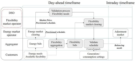
Figure 1.
Flexibility market framework (only shaded blocks are addressed by the paper).
In the Flex-DLM framework, it is assumed that the aggregator is also the energy retailer and the BRP. As an energy retailer, the aggregator participates in the day-ahead market to purchase the required energy for its customers. Once the energy market operator clears the market, the provisional schedule is sent to the DSO for technical validation. Based on such schedule, the DSO can forecast forthcoming grid contingencies occurring on the following day of operation. Consequently, a flexibility call is activated, and all aggregators are notified. The role of clearing the Flex-DLM can be carried out by a separate market entity. However, here it is assumed that this role is carried out by the DSO in order to simplify the flexibility trading process. As a result, after all aggregators submit their flexibility bids, the DSO clears the Flex-DLM and then the aggregator receives the Flex-DLM solution. The market solution should consist of the accepted flexibility bids and the time when the rebound energy can take place, thus allowing the aggregator to adjust the flexible loads accordingly. The flexibility bids modeled here (whether UREG or DREG), offered at a particular node for a trading period time , consist of a number of blocks of flexibility amounts , with different prices ordered in a non-decreasing manner, and the rebound conditions. The rebound conditions must define two main factors: the rebound hour and rebound power. The rebound hour can take place at any hour during the day, i.e., unrestricted, or it can be time restricted to a specific hour or interval. The rebound power can either be equal to or only a part of the flexibility activated. Table 3 illustrates an example for an aggregated DSF bid consisting of 3 blocks and the given possibilities of the rebound conditions. It must be remarked that the additional information required by the DSO to run this market is small compared to the amount of information the DSO is already managing.
Table 3.
Flexibility bids components.
At the moment, literature about flexibility pricing is limited. The work in [44] provided a proposal for valuing demand elasticity. In this paper, demand flexibility trading is different from the normal electricity trading in wholesale markets. In order to comply with the Flex-DLM solution, aggregators must carry out further energy trading processes in forthcoming adjustment markets to balance the energy differences arising between the energy already bought by the aggregator in the day-ahead market and the adjusted new load profile after the Flex-DLM clearing. The aggregator will be also responsible for acquiring the rebound power (payback or rebate) for its customers. Therefore, as a BRP, the aggregator takes the responsibility of trading these differences in adjustment markets. In this arrangement, demand flexibility can be regarded as a trading of service and not a trading of energy, since it is the aggregator who trades the energy in future adjustment markets. This framework differs from other approaches, for instance for insular systems [15], where the DSO directly commits the generation and makes use of the demand response to solve congestion and security problems. In the proposed Flex-DLM scheme, hence, the prices of flexibility services can be independent of the day-ahead market marginal prices. However, the flexibility prices can be affected by the level of competition between different aggregators in flexibility markets. Also, they can be limited by the maximum prices that the DSO will be willing to pay in order to avoid investing in network reinforcement. The operation scheme of the Flex-DLM limits the DSO role to clearing the Flex-DLM and choosing the optimal bids to balance its network. This is consistent with the current regulatory policies that do not allow the DSOs’ participation in energy trading. Table 4 illustrates the trading by the DSO and the aggregator across the markets involved in the proposed scheme.
Table 4.
Energy trading across markets.
4. Optimization Problem
4.1. Problem Formulation
The optimization problem modeled here aims to minimize the DSO’s total cost of acquiring DSF. The two types of flexibility considered are UREG flexibility and DREG flexibility, which can be needed for solving problems of feeder overload and overvoltages, respectively [11]. In addition, the rebound effect is taken into consideration for both types of flexibility. In accordance with Spanish electricity markets criteria, trading periods of one hour are considered. The objective function is formulated as in (1). As already mentioned, the DSO is acting as the flexibility market operator. Thus, it is the DSO’s responsibility to clear the Flex-DLM considering the constraints described in (2)–(8):
The grid constraints are represented in (2)–(5). In (2) and (3), the active and reactive power balance equations at any node in the system are modeled. In the proposed formulation, only the active power is considered as an optimization variable in the DSF bids, while the reactive power is modeled to adapt accordingly to maintain a constant power factor for each customer. The Equations (4) and (5) reflect the network’s line capacities and the voltage magnitude bounds at any given node respectively. Equation (6) provides the maximum and minimum limits for the UREG and DREG power. Finally, Equations (7) and (8) calculate the payback and rebate powers respectively as functions of the UREG and DREG power and subject to the payback and rebate coefficients and respectively. These coefficients calculate the share amount of UREG and DREG power needed at the payback and rebate hours. In addition, the payback and rebate powers are calculated for every flexibility bid activated having rebound power at time . Sets and correspond to the activated bids for the payback and the rebate at time respectively.
The optimization problem modeled here advances on earlier studies in two main areas. First, as the Flex-DLM operator, the DSO must consider the power flow equations in order to avoid activating flexibility bids that are technically infeasible. This issue has not been considered in previous work such as in [19,60]. The second area is the modelling of the rebound effect. As already mentioned, the rebound effect can be a complex problem to handle, but it is essential to be considered since it could affect the optimal market solution. This issue was absent in literature such as in [16,17,20].
4.2. Methodology
The objective function described in (1) can be challenging to solve for large networks due to the intertemporal characteristic of the rebound effect. This means that before activating a DSF bid, the DSO must first assess the possibility of further congestions occurring as a result of the rebound effect. For large networks, with possibly a considerable number of flexible customers, such complications increase exponentially, and the problem can become difficult to handle. An optimal approach to address such a problem should be able to capture the intertemporal complexities, while not being time consuming. In addition, it must ensure the technical feasibility of any activated flexibility bid and the rebound effect. Therefore, the approach carried out here divides the optimization process into two stages, in order to efficiently manage the aforementioned complexities given any number of customers. The proposed method was briefly described in [27], and it will be summarized here.
First, it is important to clarify the concept of combination of bids. In a given network, with an aggregator responsible for n number of aggregated DSF bids, there are possible combinations of DSF bids that may solve the network congestion. Each combination consists of a number of bids with activated blocks, which include their own flexibility characteristics and rebound conditions. Thus, the number of bids is directly proportional with the number of combinations. In order to narrow the search space and avoid dealing with such many possibilities, the problem is relaxed and divided into two stages. This would help reducing the execution time of the optimization problem.
● Stage 1—Preliminary Filtering
In order to narrow down the search space in the first stage, the rebound conditions are neglected when filtering through the possible combinations. Thus, the objective becomes finding all feasible combinations that can relieve the network congestion. This stage yields a preliminary group of technically feasible combinations, which will then be used in the next stage to evaluate the rebound conditions. A conventional enumerative approach of assessing all possible combinations can be used to find the preliminary group of combinations. However, this can be time inefficient for large networks. Here, a genetic algorithm (GA) is implemented as an efficient screening tool. GA uses the natural processes of survival of the fittest such as evolution, mutation, selection and crossover to efficiently filter through all possible combinations and find the feasible ones. The GA uses an optimal power flow solver in order to assess the technical feasibility of the preliminary group. Thus, it can easily eliminate all infeasible combinations that cannot solve the congestion faster than an enumerative approach. Further details about GA can be found in [61].
● Stage 2—Rebound Conditions Evaluation
The second stage carries out an evaluation process to check the feasibility of the rebound conditions and find the optimal rebound hour for the preliminary group of feasible combinations obtained from the first stage. Combinations that result into unfeasible operation at their respective rebound hours are discarded and only the technically feasible combinations are considered. Therefore, the DSO can select the optimal combination of bids with the minimum cost of activation. The evaluation process carried out at this stage uses a branch and bound (B&B) technique to find the optimal rebound hour for the activated bids in the preliminary combinations. The B&B uses an optimal power flow solver to assess the technical feasibility of the rebound conditions. It is common that B&B often starts its solution search by relaxing some of the problem constraints [62], which was applied here by reducing the search space for the second stage.
The proposed optimization approach provides two main advantages: problem scalability and integrability with any existing optimal power flow (OPF) solver. The optimization problem considered here is scalable, as the number of customers may increase significantly depending on the distribution network configuration and the congested network assets. Hence, it is crucial that the implemented method have scalability characteristics to ensure reliable performance for larger and denser distribution networks. The optimization process is modeled and integrated in MATLAB. The optimal power flow problem (OPF) in both stages are solved by means of MATPOWER [63], which is a toolbox used to solve OPF problems. The proposed methodology does not require a complicated OPF solver tool, as it is not limited to using MATPOWER, and can be integrated with any existent OPF program. Figure 2 illustrates the two stages of the optimization process.
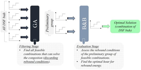
Figure 2.
Optimization methodology flowchart.
5. Case Studies
The main purpose in this section is to present the proposed Flex-DLM and to show how the two types of flexibility can contribute in the congestion management process. Two different case studies are presented to illustrate the methodology proposed for making use of UREG and DREG in the congestion management process. The case studies use real distribution feeders located in Spain. The real-life data used here are related to the overall capacities of the network lines, line parameters and the load consumptions of the network. However, the detailed information regarding the types of customers at every node and their corresponding consumption are hard to obtain, as they require communication infrastructure and data repositories. Thus, different assumptions were taken from [49,50,64], regarding the types of customers, their corresponding loads at every node and the rebound conditions for every flexibility bid. The objective is to show how the proposed methodology can handle the complexities arising from having multiple flexibility bids with different rebound conditions.
5.1. Flexibility Quantification
Before exploring the case studies, the method used to quantify the amount of available flexibility from the industrial and residential sector is explained in this subsection. In order to clarify the explanation, the number of blocks k was not considered in the subscripts since the flexibility amount intended to be calculated here corresponds to the total amount of flexibility offered by each type of customer.
● Industrial Customers
For the industrial customers, the amount of up and down flexibility regulation can be calculated following (9) and (10). The UREG power is computed as in (9), with the difference between the load at time t of service activation and the minimum load level for this customer. The DREG power is calculated in (10) with the difference between the maximum load level and the load at hour t of service activation:
● Residential Customers
Quantifying the flexibility at the residential sector can be a very complex problem due to many reasons. One of such is the massive amount of information and data required regarding every flexible appliance at every household, which can be very difficult to acquire. To overcome the lack of information and data, the load profiles of the flexible appliances are extracted from the total load profiles of the residential customers. According to [50], the average share percentage of flexible household appliances to the total consumption of the household varies between 15% to 52%. The appliances considered in this study are such as washing machines, air conditioning units, refrigerators, freezers, dryers, and space and water heating appliances. It is not common for all households to have all of these appliances; hence the share percentages vary. Next, the quantifying process of the flexibility suggested in [49,64] is adopted here, where a value called the flexible share was defined, which indicates the percentage of the flexible appliance load that can be either reduced or increased. The use of the flexible share percentage is different when it comes to evaluating the flexibility amount. The amount of flexible load that can be shifted, i.e., UREG, is calculated by multiplying the flexible share percentage by the load of the flexible appliance. Since flexible appliances are constrained by their installed capacity, the flexible share in case of DREG flexibility is multiplied by the unused capacity of the flexible appliances, which is the difference between the total installed capacity of the flexible appliances and their actual load. Therefore, the amounts of UREG and DREG for a single residential customer at a time t with flexible appliances are calculated as in (11) and (12):
5.2. Case Study I: Feeder Voltage Management by DREG Flexibility
Here, one of the small feeders of a distribution network in Spain operating at a 15 kV level is used. The feeder has six main buses: bus 1 is connected to the main grid while the load buses are 2, 3, 4 and 6. The grid’s overall capacity is 6 MW and its topology is illustrated in Figure 3. The line parameters r and x, corresponding to the per unit resistance and reactance considering a 100 MVA, 15 kV base, are as well given in Figure 3. Moreover, there is a solar PV plant connected at bus 6 with an installed capacity of 3.3 MW. In times of low load and high solar production, overvoltages may take place in the grid. This overvoltage might force the system operators to install rather expensive equipment to control the voltage levels to avoid PV generation curtailment or promote the use of smart PV inverters [65]. Another solution could be the curtailment of PV, but this is not a common approach in Spain, since renewable based generation are always given priority access in serving its output power. The solution proposed here is using DREG flexibility, which can keep the voltage levels in the permissible limits. In this feeder, two buses are assumed to be connected to customers providing flexibility: bus 3 is feeding an industrial park and bus 4 is feeding a residential area of households. The forecasted load demand and the solar PV production are illustrated in Figure 4, as well as the actual day-ahead market prices in €/MWh, which are obtained from the Spanish day-ahead electricity market [66]. It should be noted that the forecasted solar PV production, in Figure 4, represents a typical sunny and cloudless day in the area where the network exists. Also, the values presented in the graph correspond to the hourly average production and not to the instantaneous ones. The voltage limits for the system are 1 ± 0.05 p.u. The expected hours to violate the voltage limits are hours 10, 11 and 12 with voltage levels reaching 1.051 p.u. Here hour 10 will be used to demonstrate the flexibility bids construction and evaluation.
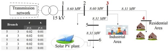
Figure 3.
Case Study I: Distribution network feeder.
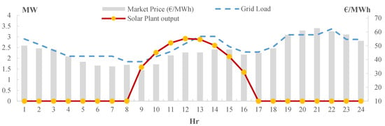
Figure 4.
Forecasted load profile (MW) and PV solar production (MW) and actual day-ahead market prices (€/MWh).
5.2.1. Creating the Flexibility Bids
The different nature of industrial and residential loads has a direct effect on the evaluation of the amount of DREG flexibility. In order to highlight these differences, every type of customer will be addressed separately to deliver a clear explanation of their effect.
● Industrial customers
The characteristics of the industrial loads are usually constrained by their production rate and economic targets. The industrial park in the given network consists of several factories that can deliver DREG flexibility, because their normal operation is beneath their full capacity. The installed capacities of these factories were obtained from [49] and fit in the load profiles of the network feeder. The amount of DREG power offered by every process in the industrial park is calculated using (10).
Table 5 presents the installed capacity for the factories considered and their loads at hour 10. Moreover, it illustrates the amount of DREG power, their corresponding prices and the rebound conditions consisting of the rebate coefficients and the time intervals for the rebate hour. The aggregated bids at that node include 4 blocks of flexibility ordered in a non-decreasing manner according to their accompanied prices. The difference in prices between the factories, as seen in Table 5, can be justified as a measure of sensitivity to the changes in the operating plan. This means that blocks offered at low prices reflect less sensitive operation to the activation of DREG flexibility. For example, the flexibility offered by is less sensitive than that of . In addition, it can be noticed that every factory is assigned to a single price. In reality, factories can be assigned to multiple prices according to the available flexibility they can offer and the sensitivity of their operation. However, assigning a single price per factory here does not affect the optimization problem nor the results.
Table 5.
Industrial area flexibility at hour 10.
● Residential customers
The residential area connected to bus 4 is assumed to have direct load control systems installed at their side that allows the aggregators to directly control the flexible loads. Aggregators are capable of bundling all the different flexible loads and accordingly constructs the flexibility bids. Moreover, it is expected that not all customers have the same standard of comfort level. While some of them are easily affected by flexibility activations, others can be less sensitive when their appliances are activated for flexibility. Therefore, the prices that the aggregators assign to the flexibility reflect the level of customers’ sensitivity to change their consumption pattern. Here, the aggregator bundles the flexibility of the residential customers into five groups, where each group shares the same standard of comfort level. The DREG power was calculated using (12), and the specific data concerning the flexible appliances were obtained from [49,64]. Table 6 presents the total load of bus 4 at hour 10, the DREG power and prices for every flexible group.
Table 6.
Industrial area flexibility at hour 10.
5.2.2. Flex-DLM Clearing
The Flex-DLM is cleared by the DSO once the aggregated bids are offered. The activated bids should decrease the voltage magnitude levels of all buses to the allowable ranges, thus alleviating any voltage constraint. In addition, the rebound conditions of these bids must not cause further network constraints during the day-ahead operation. According to Figure 4, the amount of flexibility needed to match the forecasted solar PV output at hour 10 is 0.19 MW. The activated bids for hour 10 are illustrated in Figure 5. The DSO’s optimal benefit will be activating an amount of 0.14 MW from the aggregated bid of the industrial area, which is only a part of the first block as shown in Figure 5a, and an amount of 0.06 MW from the aggregated residential bid, by full activation of the first two groups as seen in Figure 5b. The difference between the activated DREG power and the amount of flexibility originally needed accounts for the line losses taken into consideration within the formulation and the optimization procedure. Table 7 summarizes the results of the Flex-DLM for the three expected hours to suffer from overvoltage in the day-ahead operation and it provides the optimal hours for the rebate to take place. The number of the buses providing flexibility in this network is not large, therefore the complexity level here is not high and the computation time is short. However, this case study shows that DREG flexibility service can be a very useful tool for the DSO to counteract the rise of voltage levels due to the penetration of intermittent resources. In addition, since the rebate power means a decrease in the load, the DSO prefers to shift it to hours when the peak is high. For example, the first block of is activated at hour 10, and given that the rebate power can take place any time over the interval from 7 to 16, the DSO decides to move it to hour 16, which is one of the peak hours along this interval.
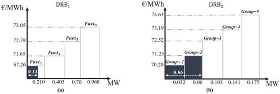
Figure 5.
(a) Activated blocks in the aggregated industrial bid at hour 10; (b) Activated blocks in the aggregated residential bid at hour 10.
Table 7.
Flex-DLM results for the day-ahead operation.
5.3. Case Study II: Feeder Overload Management by UREG Flexibility
Another distribution network feeder in Spain is used here. The area addressed consists of 79 buses with an annual demand of 109.25 GWh operating at 15 kV voltage level. This part of the grid is rather large to include its topology here. Therefore, only the part needed for this case study is depicted in Figure 6. The forecasted load profile for the day-ahead operation is illustrated in Figure 7, as well as the actual day-ahead market prices in €/MWh obtained from the Spanish day-ahead electricity market [66]. The total load profile of the grid is expected to exceed the maximum grid capacity, which is 20 MW, thus the DSO is expected to suffer from multiple outages due to overloaded lines. Instead of upgrading the grid to accommodate this increase in the load, UREG flexibility can assist the DSO in managing the grid during the hours when the load is expected to surpass the grid’s capacity. In the day-ahead operation, the hours expected to suffer from overloaded lines are 19 and 20. Hour 19 will be used to demonstrate the evaluation of UREG flexibility.
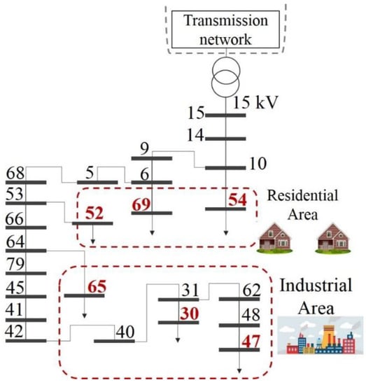
Figure 6.
Case Study II: Distribution network feeder.
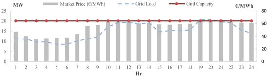
Figure 7.
Forecasted load profile (MW) and network capacity (MW) and actual day-ahead market prices (€/MWh).
5.3.1. Creating the Flexibility Bids
Similar to the previous case study, there are two main areas of the grid that can provide UREG flexibility, an industrial area and a residential area. The flexibility bids from each area can be obtained as follows.
● Industrial customers
The industrial area consists of three buses (30, 47 and 65), where every bus is feeding several industrial factories. The data regarding the factories used here were obtained from [49]. Table 8 presents the installed capacities for the factories, the loads at every bus at hour 19, and the UREG power and prices.
Table 8.
Industrial area flexibility at hour 19.
Based on [49], industrial factories can have different preferences when it comes to the rebound conditions. Since the specific data concerning the industrial factories in this network are unavailable, the rebound conditions are assumed values in order to show the merits of the proposed methodology.
● Residential customers
The residential area is situated at buses 52, 54 and 69. The households at every bus are divided into subgroups sharing the same standard of comfort level and aggregated based on their sensitivity to the activation of flexibility. Thus, households with low comfort levels have their flexibility offered at lower prices than households with higher comfort levels. The UREG flexibility bids are illustrated in Table 9, which are calculated based on the flexible appliances data obtained from [49,64], and the total load at every bus. The aggregated flexibility bid from the residential customers consists of multiple load types from different households. Similar to the industrial area, the rebound conditions for the flexibility bids are assumed in order to reflect the diversity that may arise from different flexibility appliances and to show its impact on the DSO’s final decision. As already mentioned, the assumed rebound conditions do not undermine the case study, as they can be changed according to data availability.
Table 9.
Residential area flexibility at hour 19.
It can be noticed that the UREG flexibility prices are higher than the DREG flexibility prices, which emphasizes that the flexibility services prices are not related to the actual prices of the electricity markets. The difference in prices may be due to different contracting agreements, or the high level of competition between the aggregators at both networks.
5.3.2. Flex-DLM Clearing
In this network, there are four feasible combinations of bids resulting from the first stage of the optimization process. As previously discussed in Section 4.2, their rebound conditions are not considered when obtaining the preliminary group of feasible combinations. An example for two of these combinations of bids is shown in Figure 8. Even though the total amount of flexibility activated for all the possible combinations from stage 1 are almost equal, their rebound conditions are what determine the final result. The constraint of having specific time intervals for the payback power can limit the options on the DSO. Thus, after assessing the feasibility of the rebound conditions for all the combinations in the preliminary group, including the ones presented in Figure 8, it was found that the rebound conditions of some of them were causing further network congestions at hours 11 to 14.
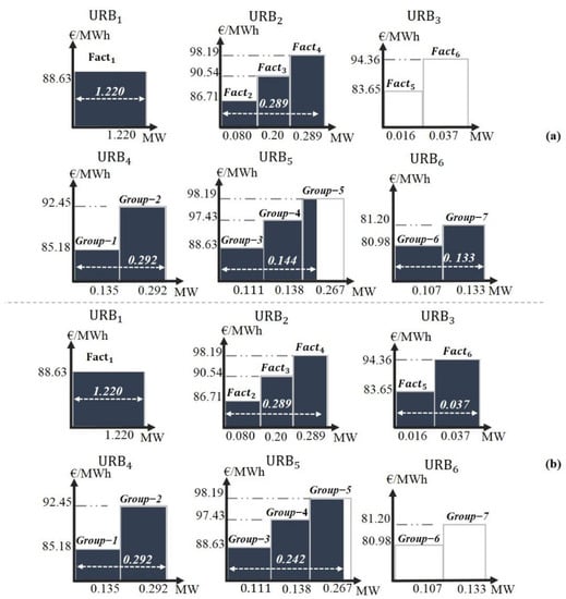
Figure 8.
Two possible feasible combinations of bids (a) and (b), resulting from stage 1 of optimization at hour 19.
The optimal combination of bids whose rebound conditions were found feasible is illustrated in Figure 9. In such combination, the whole flexibility offered in the first bid of the industrial area is activated, thus reducing the load by an amount of 1.220 MW, as seen in Figure 9a. Moreover, the flexibility from the second and third bids was activated with amounts corresponding to 0.284 MW and 0.037 MW respectively, as seen in Figure 9b,c. The first and third bids from the residential area were activated in full with amounts corresponding to 0.292 MW and 0.133 MW, as illustrated in Figure 9d,f. Only the first block from the second residential bid was activated with an amount of 0.111 MW as shown in Figure 9e. The total amount of flexibility traded at this hour corresponds to 2.07 MW, which accounts to the amount of load reduction needed by the DSO to relieve the congestion of the overloaded lines within the grid, while considering the line losses. Table 10 sums up the market results at hour 19 and 20, respectively. It presents the amount of UREG flexibility traded from every bid with its corresponding cost and the optimal hour of payback for the activated bids. As already mentioned in Section 4.2, an enumerative approach can be used for the first stage of the optimization problem, which takes approximately 16 s to solve. However, the computation time decreases by 30% when the proposed GA searching tool is used, which takes 12 s to solve. The modelling and optimization process were carried out on a CPU with Intel(R) Core(TM) i7-6700 CPU @ 3.40 GHz. Even though the given network has only 6 buses as sources of flexibility, the proposed optimization methodology is flexible to handle more buses offering flexibility, as explained in [27]. In reality, the DSO is expected to manage several feeders at the same time, where every feeder consists of hundreds of buses, which can increase the size of the optimization problem. Thus, an effective and time efficient optimization tool must be used to handle such complexity.
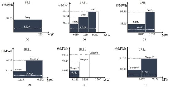
Figure 9.
Activated blocks from the industrial (a–c) and residential aggregated bids (d–f) at hour 19.
Table 10.
Flex-DLM results for day-ahead operation.
6. Conclusions
The objective of this paper is to propose a market for flexibility transactions that facilitates the trading between the DSO and the aggregators, who are bidding on behalf of their customers. The paper explains demand flexibility and classifies it into two types of flexibility namely up-regulation and down-regulation flexibility, which correspond to decreasing and increasing load volumes, respectively. Both can be valuable tools for the DSO when trying to mitigate network constraints at the distribution level. In addition, the rebound effect that is linked to both types of flexibility is defined and explained. The main stakeholders that are involved in the flexibility transactions are as well identified and their roles and responsibilities are shown. In order to ensure an effective trading for flexibility, a market for flexibility is proposed, which takes place in the day-ahead timeframe after the main wholesale market is cleared. The proposed market, named Flex-DLM, presents a simple but realistic scheme for what flexibility markets could be in the future. In addition, the Flex-DLM highlights the important role of the aggregator in maximizing the potential of demand flexibility and it does not involve the DSO in energy trading. Also, the Flex-DLM does not require complex regulatory changes which makes it easy to implement. Only the task of market clearing is assigned to the DSO, while balancing the differences between the market solutions before and after flexibility activations is assigned to the aggregator. Moreover, the proposed operation scheme of the Flex-DLM highlights the fact that demand flexibility trading should not be regarded as a trading of energy, but rather as a trading of a service.
The DSO responsibility as the Flex-DLM operator involves optimizing its purchase for demand flexibility, while ensuring that the flexibility activated alleviates the network constraints expected to occur and that the rebound conditions do not cause further network congestion. Therefore, an optimization problem is formulated that models the total cost incurred by the DSO for activating flexibility. The added value of such optimization problem is that it considers two important factors which are frequently not considered in previous literature. These two factors are the modelling of the grid power flow constraints and the complex rebound effect. The problem can be complex to handle for large networks with hundreds of customers and complex rebound conditions. The optimization methodology proposed here uses a combination of genetic algorithms and branch and bound techniques to solve the problem. Also, the proposed approach has the advantage of scalability, where it can be implemented on larger networks and its computation time is not largely affected when the problem size increase. In addition, the approach does not require complex optimal power flow solver tools to be modeled, it can be integrated with ready-made tools and a limited amount of additional information and computation capacity are needed.
Two case studies were carried out using two real distribution network feeders in Spain in order to illustrate how the proposed methodology takes advantage of the two types of demand flexibility, UREG and DREG, in the congestion management process. In the first case study, the distribution network suffers from occasional overvoltages due to the high penetration of solar PV power plant. Since the renewables are given priority access for serving their energy in Spain, the optimal solution for the DSO will not be curtailing the solar PV energy, but rather installing voltage regulators that can be expensive. The solution proposed for such problem is activating down-regulation flexibility, where load increase volumes can be procured by the DSO to sustain the voltage levels in the permissible range. Even though this case study does not have a large network, the effect of the down-regulation flexibility can be achieved as the flexibility activated assisted the DSO in managing the voltage levels of its network. The second case study highlights the value of up-regulation flexibility for the DSO in managing feeders’ overloads. The large network presented has a forecasted consumption at the day-ahead operation that is overloading some of the lines. The up-regulation flexibility offered by the customers can assist the DSO in avoiding overload congestion in the network. While there are many feasible solutions for relieving this congestion, the rebound conditions imposed further congestions in the network for some of these solutions. Thus, the optimal solution can be activated by the DSO. The proposed optimization saves a considerable amount of time as opposed to using a conventional technique.
The flexibility market proposed in this paper operates in the day-ahead timeframe. However, the grid congestions forecasted at this time might not take place and the DSO could need a different amount of flexibility. The proper consideration of the uncertainties of the forecasting process would require probabilistic optimization algorithms and a proper risk management method. This is the subject of future research.
Author Contributions
All authors were responsible for conceptualizing the framework, writing & editing and reviewing the paper; Ayman Esmat was responsible for coding and modeling the case studies.
Acknowledgments
We thankfully acknowledge the help of Unión Fenosa Distribución for the data provided for the case studies.
Conflicts of Interest
The authors declare no conflicts of interest.
Nomenclature
| Indices: | |
| j, n | Indices for nodes |
| Index for time | |
| Constants: | |
| Number of nodes in the system | |
| Number of flexibility blocks at node n at time t | |
| Optimization variables: | |
| Up/Down flexibility regulation active power in node n, at block k and hour t (MW) | |
| Other variables: | |
| Net injected active power at bus n, at hour t (MW) | |
| Net injected reactive power at bus n, at hour t (Mvar) | |
| Up/Down flexibility regulation reactive power in node n, at block k and hour t (MW) | |
| Active payback power for bus n at hour t (MW) | |
| Active rebate power for bus n at hour t (MW) | |
| Reactive payback power for bus n at hour t (MW) | |
| Reactive rebate power for bus n at hour t (MW) | |
| Apparent power flowing through line l at hour t (MVA) | |
| Voltage magnitude and angle in node n at hour t (p.u., rad) | |
| Parameters: | |
| Up/Down flexibility regulation price in node n, at block k and hour t (€/MWh) | |
| Payback coefficient at node n (p.u.) | |
| Rebate coefficient at node n (p.u.) | |
| Maximum apparent power rating of line l (MVA) | |
| Apparent power base value (MVA) | |
| Magnitude and angle of the (n,j) element of the bus admittance matrix (p.u.) | |
| Minimum and maximum value of voltage magnitude in node n (p.u.) | |
| Minimum and maximum up/down flexibility regulation power allowed in node n, at hour t (MW) | |
| Up-regulation flexibility power offered by an industrial customer at time t (MW) | |
| Down-regulation flexibility power offered by an industrial customer at time t (MW) | |
| Load of industrial customer at time t (MW) | |
| Installed Capacity of flexible load of industrial customer (MW) | |
| Minimum load level of industrial customer (MW) | |
| Maximum load level of industrial customer (MW) | |
| Up-regulation flexibility power offered by a residential customer at time t (MW) | |
| Down-regulation flexibility power offered by a residential customer at time t (MW) | |
| Total load of residential customer at time t (MW) | |
| Load of the flexible appliance of residential customer at time t (MW) | |
| Installed Capacity of flexible appliance of residential customer (MW) | |
| Flexible share of the flexible appliance of residential customer that can be used for up-regulation (%) | |
| Flexible share of the flexible appliance of residential customer that can be used for down-regulation (%) | |
References
- Fang, X.; Misra, S.; Xue, G.; Yang, D. Smart Grid—2014 the New and Improved Power Grid: A Survey. IEEE Commun. Surv. Tutor. 2012, 14, 944–980. [Google Scholar] [CrossRef]
- Gungor, V.C.; Sahin, D.; Kocak, T.; Ergut, S.; Buccella, C.; Cecati, C.; Hancke, G.P. A Survey on Smart Grid Potential Applications and Communication Requirements. IEEE Trans. Ind. Inform. 2013, 9, 28–42. [Google Scholar] [CrossRef]
- Siano, P. Demand response and smart grids—A survey. Renew. Sustain. Energy Rev. 2014, 30, 461–478. [Google Scholar] [CrossRef]
- Gelazanskas, L.; Gamage, K.A.A. Demand side management in smart grid: A review and proposals for future direction. Sustain. Cities Soc. 2014, 11, 22–30. [Google Scholar] [CrossRef]
- Behrangrad, M. A review of demand side management business models in the electricity market. Renew. Sustain. Energy Rev. 2015, 47, 270–283. [Google Scholar] [CrossRef]
- Deng, R.; Yang, Z.; Chow, M.Y.; Chen, J. A Survey on Demand Response in Smart Grids: Mathematical Models and Approaches. IEEE Trans. Ind. Inform. 2015, 11, 570–582. [Google Scholar] [CrossRef]
- Paterakis, N.G.; Erdinç, O.; Catalão, J.P.S. An overview of Demand Response: Key-elements and international experience. Renew. Sustain. Energy Rev. 2017, 69, 871–891. [Google Scholar] [CrossRef]
- Vardakas, J.S.; Zorba, N.; Verikoukis, C.V. A Survey on Demand Response Programs in Smart Grids: Pricing Methods and Optimization Algorithms. IEEE Commun. Surv. Tutor. 2014, 17, 152–178. [Google Scholar] [CrossRef]
- Smart Energy Demand Coalition (SEDC). Mapping Demand Response in Europe Today; SEDC: Brussels, Belgium, 2014. [Google Scholar]
- Aduda, K.O.; Labeodan, T.; Zeiler, W.; Boxem, G.; Zhao, Y. Demand side flexibility: Potentials and building performance implications. Sustain. Cities Soc. 2016, 22, 146–163. [Google Scholar] [CrossRef]
- Villar, J.; Bessa, R.; Matos, M. Flexibility products and markets: Literature review. Electr. Power Syst. Res. 2018, 154, 329–340. [Google Scholar] [CrossRef]
- Flexibility and Aggregation: Requirements for Their Interaction in the Market; EURELECTRIC: Brussels, Belgium, 2014.
- Nolan, S.; O’Malley, M. Challenges and barriers to demand response deployment and evaluation. Appl. Energy 2015, 152, 1–10. [Google Scholar] [CrossRef]
- Sharifi, R.; Fathi, S.H.; Vahidinasab, V. A review on Demand-side tools in electricity market. Renew. Sustain. Energy Rev. 2017, 72, 565–572. [Google Scholar] [CrossRef]
- Catalão, J.P.S. Smart and Sustainable Power Systems: Operations, Planning, and Economics of Insular Electricity Grids; Taylor & Francis: Didcot, UK, 2015. [Google Scholar]
- Song, M.; Amelin, M. Purchase Bidding Strategy for a Retailer with Flexible Demands in Day-Ahead Electricity Market. IEEE Trans. Power Syst. 2017, 32, 1839–1850. [Google Scholar] [CrossRef]
- Song, M.; Amelin, M. Price-maker bidding in day-ahead electricity market for a retailer with flexible demands. IEEE Trans. Power Syst. 2017, 33, 1948–1958. [Google Scholar] [CrossRef]
- Tveten, Å.G.; Bolkesjø, T.F.; Ilieva, I. Increased demand-side flexibility: Market effects and impacts on variable renewable energy integration. Int. J. Sustain. Energy Plan. Manag. 2016, 11, 33–50. [Google Scholar]
- Olivella-Rosell, P.; Bullich-Massagué, E.; Aragüés-Peñalba, M.; Sumper, A.; Ottesen, S.Ø.; Vidal-Clos, J.-A.; Villafáfila-Robles, R. Optimization problem for meeting distribution system operator requests in local flexibility markets with distributed energy resources. Appl. Energy 2018, 210, 881–895. [Google Scholar] [CrossRef]
- Reihani, E.; Motalleb, M.; Thornton, M.; Ghorbani, R. A novel approach using flexible scheduling and aggregation to optimize demand response in the developing interactive grid market architecture. Appl. Energy 2016, 183, 445–455. [Google Scholar] [CrossRef]
- Marinho, N.; Phulpin, Y. Economics of distributed flexibilities for the grid considering local short-term uncertainties. In Proceedings of the 2015 IEEE Eindhoven PowerTech, Eindhoven, The Netherlands, 29 June–2 July 2015; pp. 1–6. [Google Scholar]
- Roos, A.; Ottesen, S.Ø.; Bolkesjø, T.F. Modeling consumer flexibility of an aggregator participating in the wholesale power market and the regulation capacity market. Renew. Energy Res. Conf. 2014, 58, 79–86. [Google Scholar] [CrossRef]
- Spiliotis, K.; Ramos Gutierrez, A.I.; Belmans, R. Demand flexibility versus physical network expansions in distribution grids. Appl. Energy 2016, 182, 613–624. [Google Scholar] [CrossRef]
- Ceseña, E.A.M.; Good, N.; Mancarella, P. Electrical network capacity support from demand side response Techno-economic assessment of potential business cases for small commercial and residential end-users. Energy Policy 2015, 82, 222–232. [Google Scholar] [CrossRef]
- Esmat, A.; Usaola, J. DSO congestion management using demand side flexibility. In Proceedings of the CIRED Workshop 2016, Helsinki, Finland, 14–15 June 2016; pp. 1–4. [Google Scholar]
- Esmat, A.; Usaola, J.; Moreno, M.Á. Congestion management in smart grids with flexible demand considering the payback effect. In Proceedings of the 2016 IEEE PES Innovative Smart Grid Technologies Conference Europe (ISGT-Europe), Ljubljana, Slovenia, 9–12 October 2016; pp. 1–6. [Google Scholar]
- Esmat, A.; Pinson, P.; Usaola, J. Decision support program for congestion management using demand side flexibility. In Proceedings of the 2017 IEEE Manchester PowerTech, Manchester, UK, 18–22 June 2017; pp. 1–6. [Google Scholar]
- Edelenbos, E.; Togeby, M.; Wittchen, K.B. Implementation of Demand Side Flexibility from the Perspective of Europe’s Energy Directives; Concerted Actions for the Energy Efficiency Directive (EED), Renewable energy Source (RES) Directive & Energy Building Performance Directive (EPBD): Brussels, Beligum, 2015. [Google Scholar]
- Liu, G.; Tomsovic, K. A full demand response model in co-optimized energy and reserve market. Electr. Power Syst. Res. 2014, 111, 62–70. [Google Scholar] [CrossRef]
- Bergaentzlé, C.; Clastres, C.; Khalfallah, H. Demand-side management and European environmental and energy goals: An optimal complementary approach. Energy Policy 2014, 67, 858–869. [Google Scholar] [CrossRef]
- Behrangrad, M.; Sugihara, H.; Funaki, T. Integration of Demand Response Resource of Payback effect in Social Cost Minimization Based Market Scheduling. In Proceedings of the 17th Power System Computer Conference, Stockholm, Sweden, 22–26 August 2011. [Google Scholar]
- Martínez Ceseña, E.A.; Turnham, V.; Mancarella, P. Regulatory capital and social trade-offs in planning of smart distribution networks with application to demand response solutions. Electr. Power Syst. Res. 2016, 141, 63–72. [Google Scholar] [CrossRef]
- Ruester, S.; Schwenen, S.; Batlle, C.; Pérez-Arriaga, I. From distribution networks to smart distribution systems: Rethinking the regulation of European electricity DSOs. Util. Policy 2014, 31, 229–237. [Google Scholar] [CrossRef]
- Towards Smarter Grids: Developing TSO and DSO Roles and Interactions for the Benefit of Consumers; ENTSO-E: Brussels, Belgium, 2015.
- Belhomme, R.; Sebastian, M.; Diop, A.; Entem, M.; Bouffard, F.; Valtorta, G.; de Simone, A.; Cerero, R.; Yuen, C.; Karkkainen, S.; Fritz, W. Deliverable 1.1 ADDRESS Technical and Commercial Conceptual Architectures; ADDRESS Consortium: Brussels, Belgium, 2009. [Google Scholar]
- Honkapuro, S.; Tuunanen, J.; Valtonen, P.; Partanen, J.; Järventausta, P.; Heljo, J.; Harsia, P. Practical Implementation of Demand Response in Finland. In Proceedings of the 23rd International Conference on Electricity Distribution CIRED, Lyon, France, 15–18 June 2015. [Google Scholar]
- Burger, S.; Chaves-Ávila, J.P.; Batlle, C.; Pérez-Arriaga, I.J. A review of the value of aggregators in electricity systems. Renew. Sustain. Energy Rev. 2017, 77, 395–405. [Google Scholar] [CrossRef]
- Ikäheimo, J.; Evens, C.; Kärkkäinen, S. DER Aggregator Business: the Finnish Case; Technical Research Centre of Finland (VTT): Espoo, Finland, 2010. [Google Scholar]
- Koliou, E.; Muhaimin, T.A.; Hakvoort, R.A.; Kremers, R. Complexity of demand response integration in European electricity markets. In Proceedings of the 2015 12th International Conference on the European Energy Market (EEM), Lisbon, Portugal, 19–22 May 2015; pp. 1–5. [Google Scholar]
- USEF: The Framework Explained; Universal Smart Energy Framework: Arnhem, The Netherlands, 2015.
- Designing Fair and Equitable Market Rules for Demand Response Aggregation; EURELECTRIC: Brussels, Belgium, 2015.
- Torbaghan, S.S.; Blaauwbroek, N.; Nguyen, P.; Gibescu, M. Local market framework for exploiting flexibility from the end users. In Proceedings of the 2016 13th International Conference on the European Energy Market (EEM), Porto, Portugal, 6–9 June 2016; pp. 1–6. [Google Scholar]
- A Smart, Flexible Energy System; OFGEM: London, UK, 2016.
- Nordic Council of Ministers, Nordic Energy Research. Flexible Demand for Electricity and Power: Barriers and Opportunities; Nordic Energy Research: Oslo, Norway, 2017. [Google Scholar]
- Overview of the Main Concepts of Flexibility Management; CENELEC Smart Grid Coordination Group: Brussels, Belgium, 2014.
- Abdul Muhaimin, T. Electricity Market of the Future: Assessing Economic Feasibility and Regulatory Constraints for Demand Response Aggregators in Europe; Delft University of Technology: Delft, The Netherlands, 2015. [Google Scholar]
- Mohagheghi, S.; Raji, N. Managing Industrial Energy Intelligently: Demand Response Scheme. IEEE Ind. Appl. Mag. 2014, 20, 53–62. [Google Scholar] [CrossRef]
- Paulus, M.; Borggrefe, F. The potential of demand-side management in energy-intensive industries for electricity markets in Germany. Appl. Energy 2011, 88, 432–441. [Google Scholar] [CrossRef]
- Gils, H.C. Assessment of the theoretical demand response potential in Europe. Energy 2014, 67, 1–18. [Google Scholar] [CrossRef]
- Drysdale, B.; Wu, J.; Jenkins, N. Flexible demand in the GB domestic electricity sector in 2030. Appl. Energy 2015, 139, 281–290. [Google Scholar] [CrossRef]
- Mavrikas, P.; Holmgren, U. Evaluation of Demand Response Systems for Smart Grids: State of the Art, Value Potential and the Hyllie Case; Chalmers University of Technology: Göteborg, Sweden, 2013. [Google Scholar]
- Papadaskalopoulos, D.; Strbac, G. Decentralized Participation of Flexible Demand in Electricity Markets—Part I: Market Mechanism. IEEE Trans. Power Syst. 2013, 28, 3658–3666. [Google Scholar] [CrossRef]
- Papadaskalopoulos, D.; Strbac, G.; Mancarella, P.; Aunedi, M.; Stanojevic, V. Decentralized Participation of Flexible Demand in Electricity Markets—Part II: Application with Electric Vehicles and Heat Pump Systems. IEEE Trans. Power Syst. 2013, 28, 3667–3674. [Google Scholar] [CrossRef]
- Zhang, C.; Ding, Y.; Nordentoft, N.C.; Pinson, P.; Østergaard, J. FLECH: A Danish market solution for DSO congestion management through DER flexibility services. J. Mod. Power Syst. Clean Energy 2014, 2, 126–133. [Google Scholar] [CrossRef]
- Decentralized Flexibility Market; Bundesverband Neue Energiewirtschaft: Berlin, Germany, 2016.
- Decentralized Flexibility Market 2; Bundesverband Neue Energiewirtschaft: Berlin, Germany, 2016.
- Ramos, A.; De Jonghe, C.; Gómez, V.; Belmans, R. Realizing the smart grid’s potential: Defining local markets for flexibility. Util. Policy 2016, 40, 26–35. [Google Scholar] [CrossRef]
- Smart Grid Traffic Light Concept; BDEW (German Association of Energy and Water Industries): Berlin, Germwny, 2015.
- Kornrumpf, T.; Meese, J.; Zdrallek, M.; Neusel-Lange, N.; Roch, M. Economic dispatch of flexibility options for Grid services on distribution level. In Proceedings of the 2016 Power Systems Computation Conference (PSCC), Genoa, Italy, 20–24 June 2016; pp. 1–7. [Google Scholar]
- Ottesen, S.Ø.; Tomasgard, A.; Fleten, S.-E. Prosumer bidding and scheduling in electricity markets. Energy 2016, 94, 828–843. [Google Scholar] [CrossRef]
- Andre, J.; Siarry, P.; Dognon, T. An improvement of the standard genetic algorithm fighting premature convergence in continuous optimization. Adv. Eng. Softw. 2001, 32, 49–60. [Google Scholar] [CrossRef]
- Norkin, V.I.; Pflug, G.C.; Ruszczyński, A. A branch and bound method for stochastic global optimization. Math. Program. 1998, 83, 425–450. [Google Scholar] [CrossRef]
- Zimmerman, R.D.; Murillo-Sánchez, C.E.; Thomas, R.J. MATPOWER: Steady-State Operations, Planning, and Analysis Tools for Power Systems Research and Education. IEEE Trans. Power Syst. 2011, 26, 12–19. [Google Scholar] [CrossRef]
- Gils, H.C. Economic potential for future demand response in Germany—Modeling approach and case study. Appl. Energy 2016, 162, 401–415. [Google Scholar] [CrossRef]
- Abdelmotteleb, I.; Gómez, T.; Chaves-Avila, J.P. Benefits of PV inverter volt-var control on distribution network operation. In Proceedings of the 2017 IEEE Manchester PowerTech, Manchester, UK, 18–22 June 2017; pp. 1–6. [Google Scholar]
- Omie. Available online: http://www.omie.es/inicio (accessed on 31 January 2018).

© 2018 by the authors. Licensee MDPI, Basel, Switzerland. This article is an open access article distributed under the terms and conditions of the Creative Commons Attribution (CC BY) license (http://creativecommons.org/licenses/by/4.0/).