Abstract
As is well known, the high installation and operational costs of the unified power flow controller (UPFC) restrict its widespread applications in power grid. An economical “Sen” transformer (ST) that is composed of a three-phase four-winding transformer and three sets of tap changers provides similar power flow control functionality as the UPFC. Unfortunately, the ST is not suitable for high-voltage systems because of its high-voltage insulation requirement on all secondary windings and tap changers. To overcome this problem, a high-voltage “Sen” transformer that consists of a three-phase two-winding transformer and two sets of tap changers is proposed in this paper. In high-voltage power system applications, the high-voltage “Sen” transformer (HVST) offers several advantages over the ST, such as fewer windings, fewer tap changers, bigger phase-shift range, and larger power flow control region. This paper focuses on the configuration, principles, and applications of the HVST. The contrastive simulation results in a two-area test system and an IEEE 39 bus system prove the validity and advantages of the proposed HVST. Moreover, a 10 kV HVST device and a corresponding experiment platform are developed to verify the feasibility and effectiveness of the HVST. The HVST can provide a flexible voltage and power flow control.
1. Introduction
The uneven distribution of energy resources and uneven economic development lead the power grid towards a direction of high-voltage long-distance transmission systems [1]. The power flow distribution on the transmission lines is decided by the network structure and parameters. This situation is not always optimal [2]. In the bad cases, some transmission lines are overloaded, and this influences the stability of the power system [3]. Besides, for cost and environmental reasons, it is becoming increasingly difficult and time-consuming to obtain the permits to build new transmission corridors. In order to meet the increasing electricity demand, there exists an urgent need to enhance the transmission capability of the existing power grid [4,5]. To satisfy these requirements, a flexible and economic power flow controller is needed for high-voltage systems.
As a typical flexible AC transmission system (FACTS) device, a unified power flow controller (UPFC) can provide various flexible control methods for power systems [6]. The UPFC can optimize power flow distribution and increase the capacity of transmission lines [7,8]. At present, research on UPFC systems mainly focuses on improving UPFC topology configuration and enhancing power flow control functions [9,10,11]. The traditional UPFC, which is based on a voltage source converter (VSC), injects a harmonic voltage to the power system. Besides, the UPFC capacity is limited by the voltage capacity and current capacity of power electronic devices. Later, a UPFC based on the modular multilevel converter (MMC-UPFC) was proposed. The MMC-UPFC improves the waveform quality of output voltage and is suitable for large-capacity situations [12]. However, the modular multilevel structure increases the costs and the control complexity.
The phase-shifting transformer (PST) is more widely used than the UPFC in power grid for its high reliability and cost effectiveness. However, the conventional PST cannot independently adjust the active and reactive power flow of the transmission line as the UPFC does. In this case, the “Sen” transformer (ST) was proposed to improve the regulation performance of the conventional PST [13]. Detailed comparisons among ST, PST, and UPFC were made in a study [14]. This work introduced the advantages of ST in voltage regulation, power flow control, low costs, and high reliability. The ST adopts a three-phase four-winding transformer and three sets of tap changers and injects a voltage of variable magnitude and phase angle. A tap-changing algorithm for the implementation of the ST was presented in [15]. With optimized allocation, the ST can also be used for active power loss reduction [16]. A recent paper [17] presented a real-time electromagnetic transient model of the ST, which can be used for various applications, such as electromagnetic transient analyses, transformer design optimization, energy efficiency analyses, and so on. For the discrete characteristics of ST tap changers, a hybrid electromagnetic unified power flow controller (HEUPFC) was proposed. The HEUPFC consists of a big-capacity ST and a small-capacity UPFC and can control the power flow continuously [18,19].
The cost advantage of ST comes from the fact that the ST does not require an isolation transformer to inject voltage to the power system [13,14]; instead, all secondary windings and tap changers of the ST should be connected in series with the transmission line directly. Such a structure requires high-voltage insulation on all secondary windings and tap changers, and this concept is hard to realize in high-voltage systems. Another study [20] suggested that, when the system voltage level is higher than 230 kV, an additional isolation transformer should be adopted to inject ST compensating voltage. The ST is not suitable for high-voltage systems. At present, the experimental study on ST is limited to voltages lower than 110 V.
Therefore, a high-voltage “Sen” transformer (HVST) is proposed, consisting of a three-phase two-winding transformer and two sets of tap changers. In the high-voltage power system application, the HVST proposed in this paper maintains the advantages of the ST and further improves its performance. In addition, it has a simpler structure than the ST transformer. A 10 kV hardware of the HVST is developed to prove the correctness and feasibility of this method. The magnitude and phase of the HVST outputs discretely change voltages, and these voltages provide an independent active and reactive power flow control. Since the winding connection styles are different, the HVST has a larger phase-shift range and power flow regulatory region than the ST. Furthermore, a big-capacity HVST can also work with a small-capacity UPFC to provide a continuous voltage and power flow regulation as the HEUPFC does [19].
A description of the ST and of the HVST is proposed in Section 2. The HVST principle is provided in Section 3, and the comparison between the ST and the HVST is introduced in Section 4. Applied research is performed in a two-area test system and an IEEE 39 bus system in Section 5. The experimental results of a 10 kV HVST system are analyzed in Section 6. Conclusions are presented in Section 7.
2. Configuration of the HVST
To understand the configuration differences between the ST and the proposed HVST more clearly, this section introduces the winding configurations and connection modes of both the ST and the HVST.
2.1. ST Configuration [13]
The “Sen” transformer (ST) is connected to the sending end of the transmission line, as shown in Figure 1a. The ST consists of a three-phase four-winding transformer and three sets of tap changers. The three primary windings (A, B, and C) are Y connected. The transmission line voltages (UsA, UsB, and UsC) at the sending end are applied in shunt to the three primary windings. The series-compensating voltages (USTA, USTB, and USTC) come from the nine secondary windings of the ST (a1, a2, and a3 are in phase with the primary winding A; b1, b2, and b3 are in phase with the primary winding B; c1, c2, and c3 are in phase with the primary winding C). After injecting the compensating voltages (USTA, USTB, and USTC), the sending-end voltages of the transmission line are changed from UsA, UsB, and UsC to UsA1, UsB1, and UsC1:
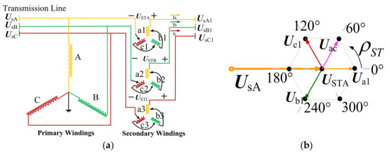
Figure 1.
“Sen” transformer (ST) configuration and output voltage. (a) ST configuration; (b) Output voltage phasor USTA.
The number of active turns in the secondary windings can be varied with the use of tap changers. It should be noted that a1, b2, and c3 are tapped at the same number of turns; b1, c2, and a3 are tapped at the same number of turns; c1, a2, and b3 are tapped at the same number of turns. However, the number of turns in the each of the three sets, a1-b2-c3, b1-c2-a3, and c1-a2-b3, can be different. Therefore, the compensating voltage becomes variable in magnitude and variable in phase angle [15].
Taking phase A as an example, the compensating voltage USTA is shown in Figure 1b. UsA is the sending-end voltage of the transmission line. The hexagonal range represents the output voltages that the ST can provide. USTA and ρSTA are the magnitude and angle of the voltage phasor USTA. When the tap positions in the secondary windings are varied, the compensating voltage becomes variable in magnitude and variable in phase angle. For example, when the tap positions in the secondary windings a1, b1, and c1 take the values of 1, 0, and 0, respectively, the output voltage USTA is equal to Ua1. When the tap positions in the secondary windings a1, b1, and c1 take the values of 1, 0, and 1, respectively, the output voltage USTA is equal to Uac.
2.2. HVST Configuration
The high-voltage “Sen” transformer (HVST) topology is shown in Figure 2. The HVST consists of a three-phase two-winding transformer and two sets of tap changers. The three primary windings (A, B, and C) are Y connected. The transmission line voltages UsA, UsB, and UsC at the sending end are applied in shunt to the three primary windings. The primary windings of the HVST have a set of tap changers. These parts of adjustable windings in the primary windings are labeled as windings a1, b1, and c1. The structure of the primary winding is similar to an autotransformer. The three secondary windings are labeled as windings a2, b2, and c2. The compensating voltages UHVSTA, UHVSTB, and UHVSTC produced by the HVST are injected in the sending end of the transmission line via a three-phase isolation transformer. The induced voltages from two different windings are combined through a series connection to produce a compensating voltage, e.g., b1 and c2 for injection in the transmission line phase A, c1 and a2 for injection in the transmission line phase B, and a1 and b2 for injection in the transmission line phase C. After injecting the compensating voltage (UHVSTA, UHVSTB, and UHVSTC), the sending-end voltage of the transmission line are changed from UsA, UsB, and UsC to UsA1, UsB1, and UsC1:
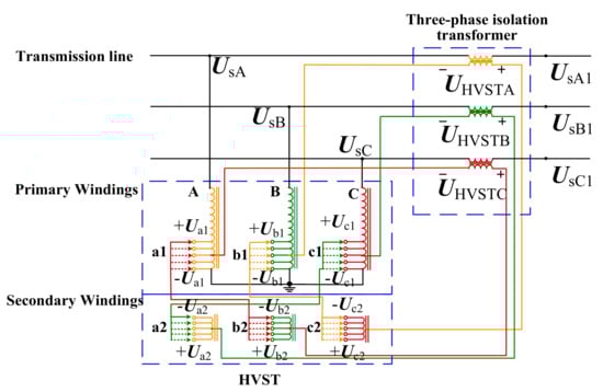
Figure 2.
High-voltage “Sen” transformer (HVST) configuration.
In the HVST, it should be noted that b1, c1, and a1 are tapped at the same number of turns; c2, a2, and b2 are tapped at the same number of turns. However, the number of turns in the b1-c1-a1 set and c2-a2-b2 set can be different. In this way, the compensated three-phase voltage (UsA1, UsB1, and UsC1) can maintain the symmetry.
To get a better look at the windings connection mode of the HVST, we show the enlarged structure of the primary winding B and secondary winding c2 in the HVST in Figure 3a. The compensating voltage UHVSTA produced by winding b1 and winding c2 is injected in the sending end of the transmission line phase A via an isolation transformer. The tap changers are adjustable at (0, ±1, ±2,···, ±m) levels. The number and direction of active turns in the winding b1 and winding c2 can be varied with the use of tap changers. Therefore, the compensating voltage becomes variable in magnitude and variable in phase angle.
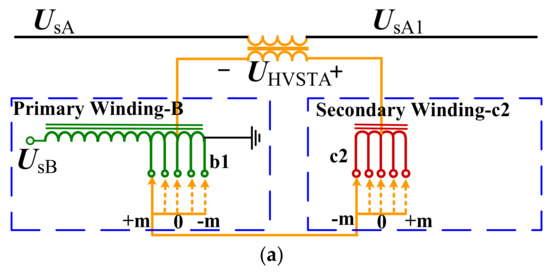
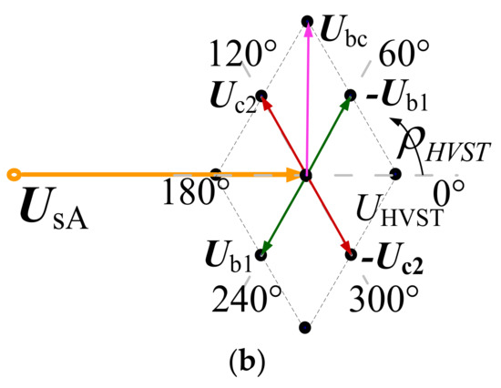
Figure 3.
HVST partial enlarged configuration and output voltage phasor. (a) Enlarged HVST configuration; (b) Output voltage phasor UHVSTA (m = 1).
The compensating voltage UHVSTA is shown in Figure 2b. UsA is the sending-end voltage of the transmission line. The rhombus range represents the output voltages that the HVST can provide. UHVSTA and ρHVSTA are the magnitude and angle of the voltage phasor UHVSTA. When the tap positions in the windings b1 and c2 are varied, the compensating voltage UHVSTA becomes variable in magnitude and variable in phase angle. For example, when the tap positions in the windings b1 and c2 take the values of 1 and 0, respectively, the output voltage UHVSTA is equal to Ub1. When the tap positions in the secondary windings b1 and c2 take the values of −1 and 1, respectively, the output voltage UHVSTA is equal to Ubc.
3. The Fundamental Principles of the HVST
In this section, the voltage and power flow regulation principles of the HVST are introduced in detail. The HVST series injected voltages are calculated for different tap numbers, and the power flow regulatory regions are calculated for various system phase angle offsets.
3.1. HVST Output Voltage Phasor
Assume the maximum output voltage magnitude of the HVST windings (winding a1, b1, c1, a2, b2, c2) is equal to ±UsN and the tap changers are adjustable at (0, ±1, ±2,···, ±m) levels. The tap positions of winding b1 and c2 are labeled kb and kc and they can fetch values of (0, ±1, ±2, ···, ±m). Ub1 step and Uc2 step are the unit voltage vectors of winding b1 and c2. Ustep is the voltage magnitude on adjacent tap changers and can be calculated as follows:
The proposed HVST uses tap changers to regulate the output voltages. When the tap changers are adjustable at (0, ±1) levels, the output voltages of HVST are shown in Figure 4a. The number of the compensating vectors is 9 (including a zero vector).
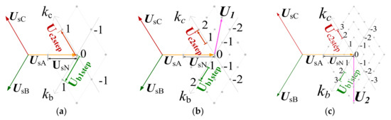
Figure 4.
HVST output voltage phasors (UHVSTA) with different tap numbers. (a) (0, ±1) level; (b) (0, ±1, ±2) level; (c) (0, ±1, ±2, ±3) level.
When the tap changers are adjustable at (0, ±1, ±2) levels, the output voltages of HVST are shown in Figure 4b. The number of the compensating vectors is 25 (including a zero vector). For example, when the tap positions in the windings b1 and c2 take the values of kb = −2 and kc = 1, the output voltage UHVSTA is equal to U1.
When the tap changers are adjustable at (0, ±1, ±2, ±3) levels, the output voltages of HVST are shown in Figure 4c. The number of the compensating vectors is 49 (including a zero vector). For example, when the tap positions in the windings b1 and c2 take the values of kb = 3 and kc = −3, the output voltage UHVSTA is equal to U2.
By that analogy, when the tap changers are adjustable under the ±m level, the number of the vectors produced by HVST is (2m + 1)2. The compensating voltage phasor produced by the HVST is calculated by (4):
The higher the number of tap changers, the higher the number of voltage vectors the HVST produces. In this way, we can adopt appropriate tap changers to obtain the more accurate output voltage value.
3.2. HVST Power Flow Control
Figure 5 shows a transmission line with the HVST block. The active and reactive power flows at the receiving end of the transmission line, Pr and Qr, are governed by the following equations:
where Us is the magnitude of the sending-end voltage, Ur is the magnitude of the receiving-end voltage, δ is the difference in phase angle between the sending-end and the receiving-end voltages, XL is the reactance of the line. UHVST and ρHVST are the magnitude and phase angle of the series voltage produced by the HVST.
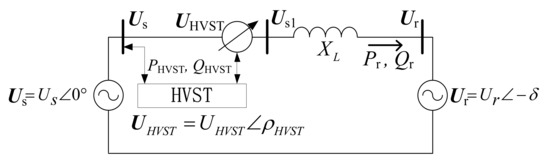
Figure 5.
Power transmission system with the HVST block.
The magnitude UHVST can be varied from 0 to , and the phase angle ρHVST can be varied from 0° to 360°, as shown in Figure 4. By changing the magnitude or the phase angle of the HVST output voltage, both the active and the reactive power flow can be regulated.
Assuming that Us = Ur = 1 pu and XL = 0.1 pu, we can get the compensated active and reactive power flows as shown in Equations (7) and (8).
For the case when the HVST rated voltage UsN is 0.3 pu and the HVST adjustment class m is 3, we can get the operating region of Pr and Qr from Equations (3)–(8). Figure 6a–d show the relationships between Pr and Qr corresponding to δ = 0°, δ = 10°, δ = 20°, and δ = 30°, respectively.
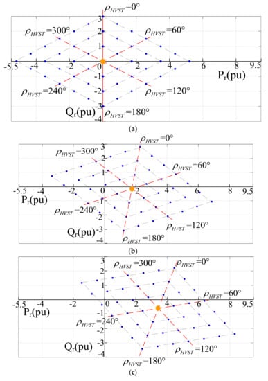
Figure 6.
Relationship between Pr and Qr with HVST regulation for different system phase angle offsets. (a) The phase difference is 0° (δ = 0°); (b) The phase difference is 10° (δ = 10°); (c) The phase difference is 20° (δ = 20°); (d) The phase difference is 30° (δ = 30°).
The center point of the rhombus is the Pr-Qr operating point without HVST compensation. The discrete points on the three rhombuses are the Pr-Qr operating points with HVST regulation. It can be seen from Figure 6 that the HVST can provide the functions of independent and bidirectional control of active and reactive power flow. The HVST can expand the Pr-Qr operating range of the power system.
The tap changer operation in an HVST provides a discrete power flow control, but it is adequate in most utility applications with appropriate HVST tap changer numbers. As the HVST can expand the power flow operating range, it has a profound effect on optimizing the system operation if an appropriate number of HVST are installed in the transmission lines.
4. Comparison between the ST and the HVST
This section compares the ST and the HVST in terms of phase-shift angle range, power flow regulatory region, and device configuration.
4.1. Phase-Shift Angle Range
Assuming the ST and the HVST have the same rated voltage (UsN), the phase-shift angles produced by the ST and the HVST are shown in Figure 7.
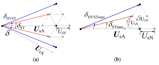
Figure 7.
The phase-shift angles of the ST and the HVST. (a) The phase-shift range; (b) The maximum phase-shift angle.
Assuming that UsA = 1 pu, we can get the maximum phase-shift angle produced by the ST and the HVST, as shown in Equations (9) and (10).
When the range of values allowed for UsN is 0 to 0.5 pu, the curves of maximum phase-shift angle produced by the ST and the HVST are shown in Figure 8.
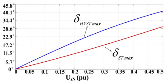
Figure 8.
The phase-shift angles of the ST and the HVST.
As we can see from Figure 8, when the rated voltage UsN of the ST and the HVST takes the same value, the maximum phase shift angle produced by the HVST is bigger than that of the ST. The HVST has a bigger phase-shift angle range than the ST.
4.2. Power Flow Regulatory Region
When the parameter δ, which is the phase difference between the sending-end and the receiving-end voltages, ranges from 0° to 30°, the reactive power flow regulatory region controlled by the ST and HVST is the same, but the active power flow regulatory region is different (Figure 6).
Figure 4 and Figure 6 show that, when the HVST output voltage takes the values of and , the active power flow at the receiving end of the transmission line reaches the maximum and minimum values, respectively. Besides, when the ST output voltage takes the values of and , the active power flow at the receiving end of the transmission line reaches the maximum and minimum values, respectively. Combining with Equation (7), we can get the maximum active power flow controlled by the HVST and the ST:
Similarly, the minimum active power flow controlled by the HVST and the ST is:
Figure 9 shows how the parameter δ and the rated voltage UsN affect the active power flow regulatory region controlled by the ST and the HVST. When the parameter δ ranges from 0° to 30° and the rated voltage UsN ranges from 0 to 0.5 pu, the maximum active power flow regulation value controlled by the HVST is always higher than that of the ST. Moreover, the minimum active power flow regulation value controlled by the HVST is always lower than that of the ST. Therefore, the HVST has a larger active power flow regulatory region than the ST.
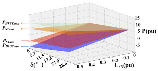
Figure 9.
The active power flow regulatory region controlled by the ST and the HVST.
Similar to the above analysis, we can get the following conclusions. When the parameter δ ranges from 30° to 60°, the HVST has a larger active and reactive power flow regulatory region than the ST; when the parameter δ ranges from 60° to 90°, the HVST has a larger reactive power flow regulatory region than the ST.
4.3. Comprehensive Comparison Between the ST and the HVST
A comprehensive comparison between the ST and the HVST is given in Table 1. In Section 4.1 and Section 4.2 the detailed analysis of the phase-shift angle range and power flow regulatory region for the ST and the HVST shows that the corresponding performance of the HVST is better than that of ST. Besides, the ST consists of a three-phase four-winding transformer and three sets of tap changers, whereas the HVST consists only of a three-phase two-winding transformer and two sets of tap changers. The HVST has a simpler structure with fewer secondary windings and fewer tap changers, which is easier to realize in engineering.

Table 1.
Comparison between the ST and the HVST.
It should be noted that when the line-to-line transmission voltage Us is lower than 230 kV, the HVST uses one more isolated transformer than the ST. In this situation, we should calculate the actual costs to determine which device is more suitable for the specific case.
When the line-to-line transmission voltage Us is higher than 230 kV, the ST also requires an isolated transformer [20]. In this situation, the HVST is more suitable in the practice than the ST.
5. Simulation
The simulation studies include two parts: the first one is a simulation comparison between the ST and the HVST in a two-area system, and the second one is a simulation comparison between the ST and the HVST in an IEEE 39 bus system.
5.1. Two-Area Test System
5.1.1. System Description
The simulation system is comprised of two AC systems which are connected by a three-phase transmission line as shown in Figure 5. The ST or the HVST is connected to the sending end of the transmission line. Table 2 gives the parameters for the ST, the HVST, and the network.
Table 2.
Simulation parameters for the ST and the HVST.
5.1.2. Simulation Results
The steady-state simulation results of the ST and the HVST obtained when the tap changers of the ST and the HVST are switched to any possible positions are shown in Figure 10.
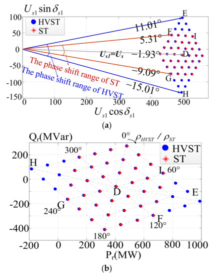
Figure 10.
The steady-state simulation results of the ST and the HVST. (a) The compensated sending-end voltage Us1; (b) The relationship between the active and reactive power flows Pr and Qr.
As we can see from Figure 10, the phase-shift angle range and active power flow regulatory region of the HVST are bigger than those of the ST. Some simulation points that the HVST can reach are beyond the control of the ST. Taking the points “D”, “E”, “F”, “G”, “H”, and “I” as examples, Table 3 shows the corresponding ST and HVST output voltages, compensated sending-end voltages, phase-shift angles, and active and reactive power flows at the receiving end of the transmission line.
Table 3.
Steady state simulation results for the ST and the HVST.
Table 3 shows that point “D” represents the system operation without ST or HVST compensation. The phase-shift angle range of the HVST is from −13.1° to 12.9° (Points “H”, “E”) and the active power flow regulatory region of the HVST is from -188 MW to 990 MW(Points “H”, “E”). The phase-shift angle range of the ST is from −7.2° to 7.3° (Points “G”, “F”) and the active power flow regulatory region of the ST is from 64 MW to 734.3 MW (Points “G”, “I”). The ST and the HVST have the same reactive power flow regulatory region.
Transient compensation is compared using the ST or the HVST. In the simulation, the ST or HVST starts to operate at 2 s. The relevant simulation parameters are shown in Table 2. The initial active and reactive power flows are 405 MW and −61 MVar. The control targets of active and reactive power flows are 900 MW and −100 MVar. Figure 11 shows the active and reactive power flows, Pr, and Qr, of the transmission system for the ST and the HVST.
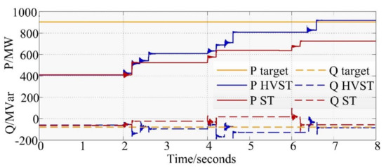
Figure 11.
The curves of power flows compensated by the ST or the HVST.
The control strategy of the HVST is similar to that of the ST [15,19]. Based on Equations (5) and (6), the required compensating voltage can be calculated according to the power flow control targets. Then, the needed tap positions of the ST and the HVST can be calculated from (1) and (2), respectively. Because of the operation characteristics of the tap changers, the ST and the HVST should adjust their tap changers from the current positions to the needed positions step by step.
The ST adjusts its tap positions (ka, kb, kc) from (0, 0, 0) to (1, 0, 1), (2, 0, 2), (2, 0, 3) in 2 s, 4 s, 6 s, respectively, to satisfy the target value. The final active and reactive power flows compensated by the ST are 711.9 MW and −65.9 MVar. The relative errors are 20.9% and 34.1%, respectively.
The HVST adjusts its tap positions (kb, kc) from (0, 0) to (−1, 1), (−2, 2), (−3, 2) in 2 s, 4 s, 6 s, respectively, to reach the target value. The final active and reactive power flows compensated by the HVST are 905.2 MW and −102.2 MVar. The relative errors are 0.6% and 2.2%, respectively. The analysis above proves that the compensation accuracy of the HVST is higher than that of the ST in some special power flow compensating zones.
5.2. Application to an IEEE 39 Bus System
5.2.1. Network Model
In this section, the ST and the HVST will be tested in an IEEE 39 bus system to illustrate the effectiveness of the HVST in a high-power system. The IEEE 39 bus system and the corresponding active power flows distribution are shown in Figure 12. The voltage base value is 330 kV.
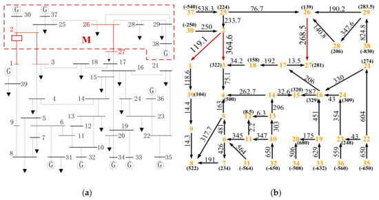
Figure 12.
The IEEE 39 bus system without any power flow control devices. (a) The IEEE 39 bus system; (b) The active power flow distribution.
In Figure 12b, the numbers 1 to 39 represent the buses of power system. The positive numbers and negative numbers in the brackets by the side of the buses represent the active loads and active power outputs, respectively. The arrows show the direction of the active flows in the transmission lines and the data on the arrows show the value of the transferred active power flows. The unit of active power is the megawatt (MW).
From Figure 12a, we can see that the area “M” transfers its active power flows to other areas only by the transmission lines 2-1, 2-3, and 26-27. The active power flows on these three lines are 119.1 MW, 364.6 MW, and 268.5 MW, respectively. They are unequally distributed. The heavy active power flow on transmission line 2-3 is a major factor limiting the power transmission capability from area “M” to other areas. Therefore, a power flow control device (the ST and the HVST) can be applied in this system to improve the active power flow distribution.
5.2.2. Simulation Results
As shown in Figure 12a, a power flow control device (the ST and the HVST) can be installed at the sending end of transmission line 2-1. When the power flow controller increases the active power flow on the transmission line 2-1, the active power flows on the transmission lines 2-3 and 26-27 will decrease simultaneously. In this way, the ST and the HVST can make the power flow distribution more reasonable. Figure 13 shows the active power flow distribution of the IEEE 39 bus system with the ST or the HVST compensation (UsN = 0.15 pu).
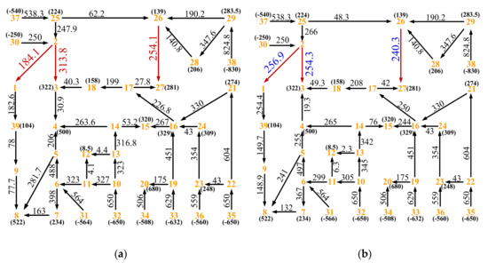
Figure 13.
The active power flow distribution of the IEEE 39 bus system with ST or HVST compensation. (a) With ST compensation (UsN = 0.15 pu); (b) With HVST compensation (UsN = 0.15 pu).
Figure 13a shows the active power flow distribution with ST compensation (UsN = 0.15 pu). In this situation, the active power flows on the three transmission lines are 184.1 MW, 313.8 MW, and 254.1 MW. The active power flow on line 2-3 is 70 percent higher than that on line 2-1. Besides, the active power flow on line 26-27 is 38 percent higher than that on line 2-1. The power flows are still unevenly distributed.
In the same simulation condition (UsN = 0.15 pu), the active power flow distribution compensated by the HVST is shown in Figure 13b. The active power flows on the transmission lines 2-1, 2-3, and 26-27 are 256.9 MW, 254.3 MW, and 240.3 MW, respectively. The active power flow difference among the three transmission lines is no more than 7 percent. They are distributed evenly. This analysis proves that the regulation capacity of the HVST is higher than that of the ST in the same rated voltage.
Figure 14 shows the transmission active power flows of lines 2-1, 2-3, 26-27 at various UsN for the ST and the HVST. The HVST can balance the active power flows on three lines when the rated voltage UsN is 0.15 pu. However, for the ST, the active power flows on three lines can be balanced when the UsN is around 0.3 pu. In this IEEE 39 bus simulation system, the ST needs twice the rated voltage to achieve the same regulation effect of the HVST.
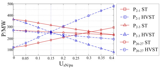
Figure 14.
The transmission active power flows of lines 2-1, 2-3, 26-27 at various UsN for the ST and the HVST.
Table 4 gives the corresponding parameters for the ST and the HVST. When the ST is applied in the high-voltage power system (Us = 330 kV), the ST also requires an isolated transformer to move the secondary windings and the tap changers to a lower voltage level [20]. In this situation, the ST does not keep its main advantage, which is that it does not require an isolated transformer. From Table 4, we can see that the HVST can balance the power flows on the three transmission lines with fewer secondary windings and fewer tap changers. Compared the ST-2 (UsN = 0.3 pu) with the HVST (UsN = 0.15 pu), the cost of the secondary windings of the HVST can be reduced by 67% and that of the tap changers of the HVST can be reduced by 33%.
Table 4.
Simulation parameters for the ST and the HVST in an IEEE 39 bus system.
6. Experiment
To validate the voltage regulation and power flow control performance of the HVST, a 10 kV HVST device and the corresponding experimental platform have been developed.
6.1. Experimental Platform
The 10 kV HVST device and the corresponding experimental platform are shown in Figure 15a,b. Figure 15c shows the corresponding equivalent circuit of this experimental platform. The reactance XL is used to simulate the transmission line. The potential transformer (PT) and current transformer (CT) are used to obtain the measuring voltage and measuring current.
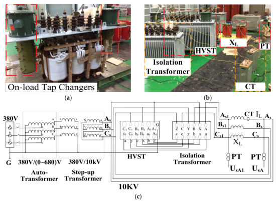
Figure 15.
The 10 kV HVST device and the corresponding experimental platform. (a) The HVST before encapsulation; (b) The experimental platform; (c) The equivalent circuit of the experimental platform.
The main parameters for this experiment are given in Table 5.
Table 5.
Experiment parameters for the HVST.
6.2. Experimental Results
Figure 16a,b show that the HVST tap changers positions (kb, kc) are tapped at (0, 0) and (−2, 2), respectively. The CH1 waveform shows the line current IL, the CH3 waveform shows the sending-end voltage UsA, the CH4 waveform shows the compensated sending-end voltage UsA1, and the Math waveform shows the HVST output voltage UHVSTA.
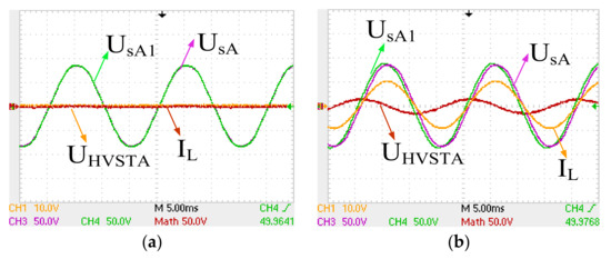
Figure 16.
Experimental waveforms of the HVST operating at different tap positions. (a) Tap position at (0, 0); (b) Tap position at (−2, 2).
In Figure 16a, the HVST output voltage UHVSTA is 0 V, so the compensated sending-end voltage UsA1 is equal to the original sending-end voltage UsA. The CH3 and CH4 waveforms almost completely coincide. In this case, the load current and the power flow on the transmission line are 0.
As shown in Figure 16b, the HVST output voltage UHVSTA is 982.1∠90° V and the original sending voltage UsA is 6000∠0° V. After the HVST compensation, the compensated sending-end voltage UsA1 changes to 6081∠9.4° V. The load current is 4.9 A. In this case, the active and reactive power flows at the receiving end of the transmission line are 26.3 kW and 0.03 kVar. This experiment proves the viability and effectiveness of the HVST for phase shifting and power flow controlling.
Figure 17 shows the experimental results when the HVST switches at all possible tap changers positions. Pr0 and Qr0 are the power flows without HVST compensation. The active power flow can be adjusted from −52.9 kW to 52.2 kW, and the reactive power flow can be adjusted from −30.5 kVar to 30.2 kVar by the HVST compensation. The results show that the HVST is a flexible and effective device to control the active and reactive power flows on the transmission line.
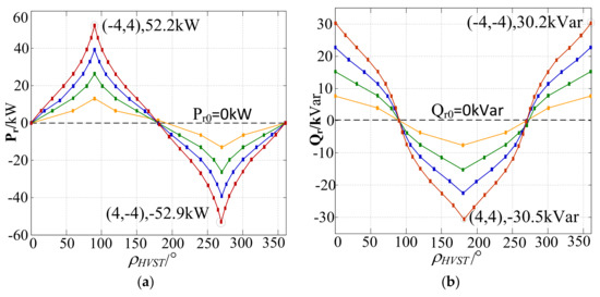
Figure 17.
The Pr and Qr experimental results at a varying series voltage (UHVST) and phase angle (ρHVST) for the HVST. (a) The active power flow Pr; (b) The reactive power flow Qr.
7. Conclusions
This paper presents a high-voltage “Sen” Transformer (HVST), which can provide independent and bidirectional active and reactive power flow control in high-voltage power systems. The structure, operational principles, and power flow regulation principles are analyzed. The simulations in a two-area test system and an IEEE 39 bus system have been used to prove the effectiveness and advantages of the HVST. Besides, a 10 kV HVST device and an experimental platform have been developed to test the phase shift and power flow control performance. The experimental results demonstrate the feasibility and effectiveness of the HVST.
Compared with the ST, the HVST has the following features: (1) The three-phase two-winding HVST with two sets of tap changers is simpler in structure than the three-phase four-winding ST with three sets of tap changers. The HVST utilizes the primary winding of the transformer to provide a partial series regulation voltage; (2) When the ST and the HVST have the same rated voltage, the HVST has a bigger phase-shift range and power flow regulatory region than the ST; (3) The HVST needs to adopt an isolation transformer to inject a series compensating voltage. The ST uses the isolation transformer only when the line-to-line voltage reaches 230 kV. When the system voltage is lower than 230 kV, the HVST uses one more isolated transformer than the ST. Therefore, the HVST has more value in industrial applications at a high-voltage level (230 kV).
Acknowledgments
This work was supported in part by the HydroChina Huadong Engineering Corporation Limited research project No. HNKJ16-H25.
Author Contributions
This article has five authors: Baichao Chen, Wenli Fei, and Cuihua Tian conceived and designed the research method and performed the experiments; Wenli Fei, Lingang Yang and Jianwei Gu analyzed the data; Wenli Fei wrote the paper.
Conflicts of Interest
The authors declare no conflict of interest.
References
- Samorodov, G.; Kandakov, S.; Zilberman, S.; Krasilnikova, T.; Tavares, M.C.; Machado, C.; Li, Q. Technical and economic comparison between direct current and half-wavelength transmission systems for very long distances. IET Gener. Transm. Distrib. 2017, 11, 2871–2878. [Google Scholar] [CrossRef]
- Miao, J.; Zhang, N.; Kang, C.; Wang, J.; Wang, Y.; Xia, Q. Steady-state power flow model of energy router embedded AC network and its application in optimizing power system operation. IEEE Trans. Smart Grid 2017. [Google Scholar] [CrossRef]
- Choudekar, P.; Sinha, S.K.; Siddiqui, A. Transmission line efficiency improvement and congestion management under critical contingency condition by optimal placement of TCSC. In Proceedings of the India International Conference on Power Electronics, Patiala, India, 17–19 November 2016. [Google Scholar] [CrossRef]
- Gajbhiye, R.K.; Naik, D.; Dambhare, S.; Soman, S.A. An expert system approach for multi-year short-term transmission system expansion planning: An Indian experience. IEEE Trans. Power Syst. 2008, 23, 226–237. [Google Scholar] [CrossRef]
- Arevalo, F.; Cordova, M.; Quizhpi, F.; Vivar, M. Genetic algorithm for enhancing the transmission capacity of a PES (power electric system) through flexible AC compensators. In Proceedings of the IEEE Conference on Industrial Electronics and Applications, Hangzhou, China, 9–11 June 2014. [Google Scholar] [CrossRef]
- Hingorani, N.G.; Gyugyi, L. Understanding FACTS: Concepts and Technology of Flexible AC Transmission Systems, 1st ed.; IEEE: New York, NY, USA, 2000; pp. 1–35, 0-7803–3455-8. [Google Scholar]
- Hao, J.; Shi, L.B.; Chen, C. Optimising location of unified power flow controllers by means of improved evolutionary programming. IEE Proc. Gener. Transm. Distrib. 2004, 151, 705–712. [Google Scholar] [CrossRef]
- Song, P.E.; Xu, Z.; Dong, H. UPFC-based line overload control for power system security enhancement. IET Gener. Transm. Distrib. 2017, 11, 3310–3317. [Google Scholar] [CrossRef]
- Liu, Y.; Yang, S.; Wang, X.; Gunasekaran, D.; Karki, U.; Peng, F.Z. Application of transformer-less UPFC for interconnecting two synchronous AC grids with large phase difference. IEEE Trans. Power Electron. 2016, 31, 6092–6103. [Google Scholar] [CrossRef]
- Albatsh, F.M.; Mekhilef, S.; Ahmad, S.; Mokhlis, H. Fuzzy-logic-based UPFC and laboratory prototype validation for dynamic power flow control in transmission lines. IEEE Trans. Ind. Electron. 2017, 64, 9538–9548. [Google Scholar] [CrossRef]
- Zahid, M.; Chen, J.; Li, Y.; Duan, X.; Lei, Q.; Bo, W.; Mohy-ud-din, G.; Waqar, A. New Approach for Optimal Location and Parameters Setting of UPFC for Enhancing Power Systems Stability under Contingency Analysis. Energies 2017, 10, 1738. [Google Scholar] [CrossRef]
- Li, P.; Lin, J.; Kong, X.; Wang, Y. Application of MMC-UPFC and its performance analysis in Nanjing Western Grid. In Proceedings of the IEEE PES Asia-Pacific Power and Energy Engineering Conference, Xi’an, China, 25–28 October 2016. [Google Scholar] [CrossRef]
- Sen, K.K.; Sen, M.L. Introducing the family of “SEN” Transformer: A set of power flow controlling transformers. IEEE Trans. Power Deliv. 2003, 18, 148–157. [Google Scholar] [CrossRef]
- Sen, K.K.; Sen, M.L. Comparison of the “SEN” Transformer with the unified power flow controller. IEEE Trans. Power Deliv. 2003, 18, 1523–1533. [Google Scholar] [CrossRef]
- Faruque, M.O.; Dinavahi, V. A tap-changing algorithm for the implementation of “SEN” transformer. IEEE Trans. Power Deliv. 2007, 22, 1750–1757. [Google Scholar] [CrossRef]
- Mohamed, S.E.G.; Jasni, J.; Radzi, M.A.M.; Hizam, H.; Mirzaei, M. Optimal allocation of Sen transformer for active power loss reduction. In Proceedings of the IEEE International Conference on Power and Energy, Kuching, Malaysia, 1–3 December 2014. [Google Scholar] [CrossRef]
- Liu, J.; Dinavahi, V. Nonlinear magnetic equivalent circuit based real time Sen transformer electromagnetic transient model on FPGA for HIL emulation. IEEE Trans. Power Deliv. 2016, 31, 2483–2493. [Google Scholar] [CrossRef]
- Yuan, J.; Chen, L.; Chen, B.C. The improved Sen transformer—A new effective approach to power transmission control. In Proceedings of the IEEE Energy Conversion Congress and Exposition, Pittsburgh, PA, USA, 14–18 September 2014. [Google Scholar] [CrossRef]
- Yuan, J.; Liu, L.; Fei, W.; Chen, L.; Chen, B.C.; Chen, B. Hybrid electromagnetic unified power flow controller: A novel flexible and effective approach to control power flow. IEEE Trans. Power Deliv. 2017. [Google Scholar] [CrossRef]
- Sen, K.K.; Sen, M.L. Unique capabilities of Sen transformer: A power flow regulating transformer. In Proceedings of the IEEE Power and Energy Society General Meeting, Boston, MA, USA, 17–21 July 2016. [Google Scholar] [CrossRef]
© 2018 by the authors. Licensee MDPI, Basel, Switzerland. This article is an open access article distributed under the terms and conditions of the Creative Commons Attribution (CC BY) license (http://creativecommons.org/licenses/by/4.0/).