Abstract
Wind-diesel hybridization has been emerging as common practice for electricity generation in many isolated power systems due to its reliability and its contribution in mitigating environmental issues. However, the weakness of these kind of power systems (due to their small inertia) makes the frequency regulation difficult, particularly under high wind conditions, since part of the synchronous generation has to be set offline for ensuring a suitable tracking of the power demand. This reduces the power system’s ability to absorb wind power variations, leading to pronounced grid frequency fluctuations under normal operating conditions. This paper proposes some corrective actions aimed at enhancing the frequency control capability in weak and isolated power systems: a procedure for evaluating the system stability margin intended for readjusting the diesel-generator control gains, a new wind power curtailment strategy, and an inertial control algorithm implemented in the wind turbines. These proposals are tested in the San Cristobal (Galapagos Islands-Ecuador) hybrid wind-diesel power system, in which many power outages caused by frequency relays tripping were reported during the windiest season. The proposals benefits have been tested in a simulation environment by considering actual operating conditions based on measurement data recorded at the island.
1. Introduction
Historically, stand-alone diesel power generation has shown to be the most suitable solution for electrification in remote populated areas and islands, due to its reliability and its quick installation [1]. However, burning diesel fuel for that purpose might be expensive and contribute to the emission of greenhouse gasses and to local pollution. In order to tackle these drawbacks, many countries have raised policies and incentives aimed at promoting the integration of alternative power generation technologies, mainly based on the use of renewable energy resources. In this sense, wind-diesel hybridization has been emerging as common practice in many weak and isolated power systems in last years [2]. In such kind of systems, diesel generators are able to correct the power imbalances caused by the load variation as well as the fluctuating nature of wind power. Nevertheless, during high wind condition periods, the grid frequency control could be a challenging task, which deserves special treatment compared to that given to large power systems. In many cases, the system operator could force to limit part of the available wind power in order to preserve an adequate frequency regulation margin to face any frequency event, for example, caused by a sudden loss of power generation [3,4,5]. This procedure, also called wind power curtailment, is necessary since modern wind turbines incorporate a grid connection interface based on power electronics, and do not provide inertia to the system as the conventional synchronous generators actually do in a natural manner. When the penetration of wind energy increases, the inertial response of the system tends to degrade progressively, which represents a threat for the power supply continuity [6]. Real situations that confirm the aforementioned technical difficulties took place in the San Cristobal Island hybrid wind-diesel power system (SCHPS), located at the Galapagos Islands-Ecuador, where the high participation of wind energy in the load sharing caused partial and total power outages during the windiest season of 2015. These events were caused by the tripping of certain frequency relays installed to protect the generation units. Given the seriousness of that situation, it has been found interesting to consider such power system as a case of study in this work.
Nowadays, it is possible to find in the literature many scientific contributions aimed to face the technical issues associated with the significant integration of wind turbines into small power systems. For instance, works presented in [6,7,8,9,10,11] propose the use of additional energy storage systems such as batteries, ultra-capacitors, and flywheels, in order to absorb the fluctuating nature of the power injection from wind and, therefore, to reduce the induced frequency deviations in the grid. Although these solutions have proven to be the most effective, from a technical perspective, the costs associated with their installation and maintenance could constitute a drawback to consider. On the other hand, there are also control strategies that focused on taking advantage of the available kinetic resources existing in the wind turbines in order to enable the frequency support provision while avoiding additional hardware installation. These contributions, as in [12,13,14,15,16], are conceived to provide a variable speed wind turbine with a suitable inertial response to support the grid frequency in normal operating conditions and in case of contingency. Since these strategies force the wind turbine to operate under non-optimal conditions, the cost of the wind energy waste could represent a clear disadvantage. However, many grid codes consider the possibility of sacrificing part of the generated energy in order to safeguard the quality, stability, reliability and continuity of the power supply [17,18]. This paper presents some proposals aimed at enhancing the frequency response of a weak and isolated power system with a significant share of wind energy by using the approach offered by the second group of solutions, that is, by leveraging the existing equipment installed in the system.
The first contribution of this paper is to present a procedure for evaluating the stability margin of the power system based on the classical root-locus analysis in order to foresee the consequences of manipulating certain parameters of the diesel-engine speed governors in the grid frequency response. From the previous analysis, an adjustment of the speed governor gains towards improving the frequency support capability from conventional generators is suggested. The proposed procedure is based on the conventional generation only, since variable-speed wind turbines do not provide, in principle, inertial response to the grid. Next, to go beyond this approach, the solutions proposed below are intended to make it possible for the wind turbine to mitigate its negative effects to the grid, and are designed to be implemented in its power controllers.
The second improvement proposal, which constitutes the main contribution of this paper, consists in a new wind power curtailment strategy with better benefits compared to those strategies based on the pitch angle regulation. This approach proposes the combined use of electromagnetic and mechanical variables to perform an effective wind power limitation. This results in an almost constant power injection to the grid when the available wind power exceeds a maximum limit established by the system operator, leading to a significant reduction of the grid frequency fluctuations under wind curtailment conditions.
Complementarily, in order to get a milder evolution of the grid frequency in those intervals where the wind energy is delivered under the criterion of optimal conversion (non-curtailment condition), the implementation of an inertial control based strategy in the wind turbine controllers is presented as a third corrective action. Such strategy enables the participation of the variable-speed wind turbines in the grid frequency support in cooperation with the conventional synchronous generation under normal operating conditions and under contingency scenarios.
This paper is organized as follows: Section 2 introduces the description and modeling of the SCHPS along with its implementation in MATLAB/Simulink®. All the proposals devised to enhance the frequency control tasks by the test power system when it is subjected to normal operating conditions are presented in Section 3. In order to assess the effectiveness of the improvement proposals under more critical operating conditions, Section 4 presents a detailed study of the test system when it experiences a frequency event caused by a sudden loss of wind power. Finally, the most relevant conclusions are established in Section 5.
2. Power System under Study
2.1. Description and Modeling
Figure 1a shows the configuration of the hybrid wind-diesel power system of San Cristobal Island. The conventional power plant consists of three 813 kVA-synchronous generation units (DG1, DG2, and DG3), each coupled to a diesel engine. These units inject the produced energy to a three-phase 13.2 kV bus of the distribution substation (DSS) located in the courtyard of the diesel power plant. From the DSS, three primary feeders distribute the distribution of the generated energy at different consumption points of the island. The San Cristobal wind farm, located 12 km from the DSS, is composed of three 800 kW-full converter wind turbines (WT1, WT2, and WT3) whose delivered energy is dispatched to the DSS through a 13.2 kV transmission line. Table 1 provides some relevant parameters from the nameplate of individual generation units installed at SCHPS.
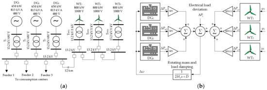
Figure 1.
Wind-diesel hybrid power system of San Cristobal Island: (a) Layout diagram; (b) Load frequency control scheme.

Table 1.
Dataset of generation units.
The load frequency control (LFC) scheme that represents the short-term behavior of frequency and power of the SCHPS is depicted in Figure 1b. That scheme is derived from the swing equation of a synchronous generator (1) [19]. In this equation, that considers small deviations of power and rotor speed, the inertial characteristics of the synchronous generators are described by the equivalent constant of inertia, HT. The electric load is characterized by its deviation ΔPL from its pre-disturbance value and its damping effect, D. Δω is the equivalent synchronous rotor speed deviation, which is equivalent to the grid frequency deviation, Δf, if both are expressed in per unit. ΔPm is the mechanical power deviation introduced by the speed governor in response to a grid frequency change Δf, and ΔPg denotes the deviation of the active power injected by the wind turbine. v is the horizontal component of wind speed incoming to the wind rotor.
The factors wi are the energy share weights and represent the ratio between the i-th synchronous generation unit capacity and a specified base power. Complementarily, wNSi are the energy share weights from the non-synchronous generation units (variable-speed wind turbines, in this case) whose definition is similar to wi. The use of these factors allows the expression of all the power deviation signals from the generation units in the same per unit base chosen for the whole power system. However, as it is expressed in (2), only the factor wi must be considered for the evaluation of HT. In this definition, Hi is the constant of inertia of each synchronous generation unit computed in its own base power, and m is the total number of online synchronous generators.
The model that represents the time-domain behavior of the diesel generation unit has been taken from [20] and schematized in Figure 2, where ωr is the rotor shaft speed, Tm denotes the mechanical torque, and Pm is the mechanical power. Tmax and Tmin are the mechanical torque limits, Pm0 is the pre-disturbance value of Pm, and ΔPm is the mechanical power deviation.
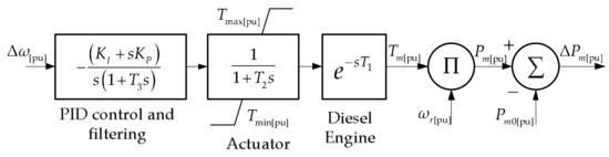
Figure 2.
Simplified model of the diesel generation unit.
In addition, the general scheme of the wind turbine model installed at the San Cristobal wind farm is shown in Figure 3a. A three-blade wind rotor is coupled to a two pole-pairs synchronous generator throughout a gearbox. The stator windings of the electrical generator are connected to the grid via a back-to-back power electronics converter (PEC). The decoupling provided by the DC-link allows the wind turbine to operate with variable speed regardless the grid frequency value. The PEC consists of two converters: Machine Side Converter (MSC) and Grid Side Converter (GSC) [21]. The MSC controls the active power delivered by the synchronous generator following a maximum power point tracking (MPPT) characteristic, which is devised to maximize the mechanical power extraction by the turbine, while the GSC regulates both the DC-link voltage and the output reactive power at the grid connection point [22]. Finally, the rotor of the synchronous generator is excited by an external DC power supply.
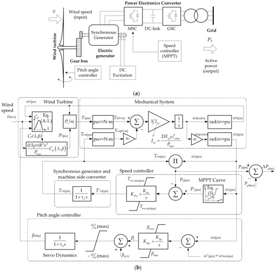
Figure 3.
Wind turbine installed at the San Cristobal wind farm: (a) General layout; (b) Simplified electro-mechanical model.
In order to represent the short-time dynamics of the variable speed wind turbine, the simplified electromechanical model proposed in [23] and depicted in Figure 3b has been used. This model, originally designed for a doubly-fed induction generator based wind turbine, can be applied to represent a wind turbine with a synchronous generator via full converter due to the similarities between their mechanical topologies and because, within the time frame considered in the load frequency control studies, the electromagnetic time constants are negligible compared to the mechanical ones. This fact allows to represent the dynamics of the power electronic converter and the electrical generator by a first order transfer function with time constant τC. In Figure 3b, Tt and Tem are the mechanical and the electromagnetic torque, respectively. Pg is the total output active power, ωt and ωg are the angular speed of the turbine and the electric generator, and β denotes blade pitch angle. Pg0 and ΔPg are the pre-disturbance value and the deviation of the output active power, respectively. The variables with the superscript * represent their set-point values. The rest of parameters of both models are defined in the Appendix.
Based on commercial datasheets and real data recorded in field tests performed at the SCHPS, all the parameters of those models have been assigned and tuned in order to represent, in a reliable way, the actual power system performance. Figure 4 shows the power curves particularized for the commercial wind turbine model. In this illustration, the MPPT curve is also plotted, whose analytical representation is expressed in (3). In this equation, Kopt is the optimization constant which depends on constructive characteristics of the wind rotor, and Pmax is the maximum active power to be delivered by the wind turbine. The different operating zones of the wind turbine along with their associated parameters are graphically defined in Figure 4a. Appendix contains all the numerical data necessary for the evaluation of (3).
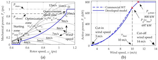
Figure 4.
Wind turbine power curves: (a) ω-P chart; (b) Power-wind speed curve.
The models depicted in Figure 2 and Figure 3 were validated by considering some real contingency situations in the studied power system. For instance, Figure 5 shows the time domain behavior of some variables recorded in the SCHPS as a consequence of a sudden loss of 700 kW of wind energy caused by the intentional disconnection of wind turbines WT1 and WT2. Such disturbance was introduced elapsed 18 s from the beginning of data recording. Prior to the contingency, the electric load was supplied only by the machines: DG1, DG2, WT1, and WT2, whose active power values are provided in Table 2. During the time frame covered by the data acquisition, the actual demanded power hardly experiences any variation, hence, this variable will be kept unchanged along the time domain simulation (ΔPL = 0).
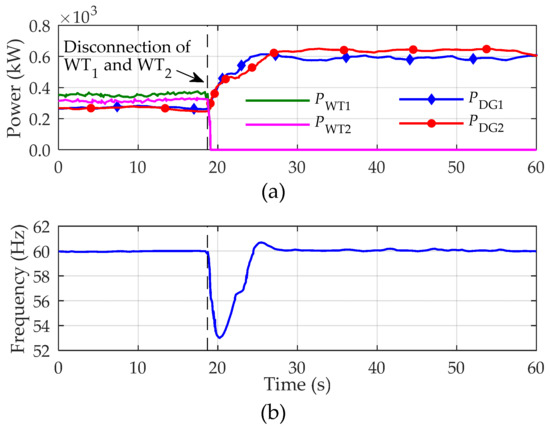
Figure 5.
Real contingency scenario at the SCHPS: (a) Power generation; (b) Grid frequency.
Table 2.
SCHPS real contingency scenario.
For the implementation of the LFC-scheme in MATLAB/Simulink®, the set of values assigned to the parameters of the speed governor of diesel-generation units has been replicated on the three thermal machines, for simplicity. Therefore, an identical response of the power and rotor speed is expected for DG1–DG3 under both normal operation and contingency. A similar reasoning has been applied to the model parameters of the wind turbines WT1–WT3. The base power for per unit calculation is chosen as the total installed capacity of the diesel power plant (Sbase = 3 × 813 kVA), so, the energy share factors will be w1 = w2 = w3 = 1/3 and wNS1 = wNS2 = wNS3 = 0.328. Table 2 presents relevant information for the representation of this specific contingency scenario, where the generators DG3 and WT3 remain offline. The time domain behavior of the variables of interest recorded in the real power system and that obtained in simulation are compared in Figure 6. Note that, it exists a high correlation, in amplitude and time, between the response of grid-frequency and total active power of the wind turbine. The similarities between the curves obtained by simulation and from real measurements allow to validate the SCHPS model presented in this section.
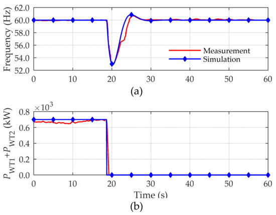
Figure 6.
SCHPS model validation: (a) Grid frequency; (b) Wind farm generated power.
2.2. Operation and Control
According to the proceeding manual of the SCHPS, the total active power produced by the wind farm, PWF, is regulated by a wind farm controller (WFC) structure as it is shown in Figure 7a. Two criteria are used for dispatching the energy production of the wind farm: ecological and technical. For addressing the first, the active power reference signal, P*WF, is set so that the power demand can be supplied by both the wind farm and the diesel power plant by burning the least possible fossil-fuel. For preserving the efficiency and lifespan of the diesel-engines, it is desirable that they operate above their minimum mechanical power, Pm,min, defined about 25% from its rated value. The total number of online diesel generators is denoted by nDG.
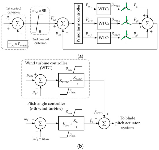
Figure 7.
Wind farm controller structure: (a) General scheme; (b) Implementation of the WTC.
For meeting the second criterion, it is expected that each online diesel generator must be able to withstand a sudden loss of wind power by using its spinning reserve (SR) to preserve the power system stability. In the SCHPS, the power reserve is calculated as: SR = (Pnom − Pm,min). For implementing this criterion, a saturation block is added to the control scheme and its output is applied to the WFC. The WFC sends a maximum active power reference, Pset, to the i-th wind turbine controller (WTC). The WTC uses the pitch angle, βWTC, as a control variable in order to limit the wind power captured by the i-th turbine. This signal is applied to the blade pitch angle controller of each wind turbine as Figure 7b illustrates. If the actual total wind power production is below its maximum specified value, each wind turbine is required to operate according to a MPPT-characteristic to extract the optimal power from wind.
2.3. Simulation of the SCHPS under Normal Conditions
The historical dispatching records of the SHSC reveal that between June and September there is a surplus of wind energy production every year [24]. In a particular case, high favorable wind conditions were registered in the San Cristobal wind farm on August 2015. This condition led wind turbines to cover the energy needs of the island up to 66% under the maximum demand scenario (PLmax = 2424 kW). During the same period, several unplanned power outages were reported. These were mainly caused by the trip of certain frequency protection relays both in the wind farm and in the diesel power plant, by causes still unknown by the operators. Given the technical seriousness of these events, such scenario will be taken as the main case of study in this work. Table 3 and Table 4 list relevant information concerning to the real status of the SHSC for the scenario described above, that approximately corresponds to the highlighted point in the wind speed profile shown in Figure 8. This illustration was generated by using real data measured at the hub height of the wind turbines (51 m) under gusty conditions.
Table 3.
SCHPS power production *.
Table 4.
SCHPS power consumption *.
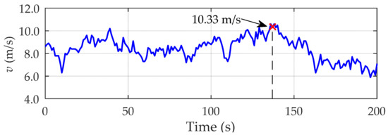
Figure 8.
Actual wind speed profile used in the time domain simulations.
For the reproduction of this case of study in MATLAB/Simulink®, the numerical value of all the parameters of both the conventional power plant and the wind farm have been assigned by using the same criteria than in Section 2.1. Nevertheless, in this case, the three synchronous generation units are online, leading to have an equivalent constant of inertia of HT = 3 × 0.4208 s. Additionally, the geographic distribution of the wind turbines, wake effect and wind transportation delay are neglected in the simulation, so, the wind profile of Figure 8 is applied simultaneously to the three wind turbines. According to the procedure described in Section 2.2., the set-point value P*WF for this specific case, which corresponds to a wind curtailment situation, is established as follows:
- First control criterion:
- Second control criterion:
- WFC active power set-point:
Figure 9a shows the active power dispatched by each wind turbine obtained by simulation. The total power injected by the wind farm into the grid is illustrated in Figure 9b, along with the theoretical optimal wind power which is not dispatched due to the activation of the curtailment operation mode in the WFC.
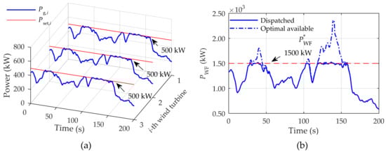
Figure 9.
Dispatched active power: (a) Wind turbines; (b) Wind farm.
Finally, the simulated dynamics of the active power delivered by the SCHPS generation agents and the grid frequency are shown in Figure 10 and Figure 11, respectively.
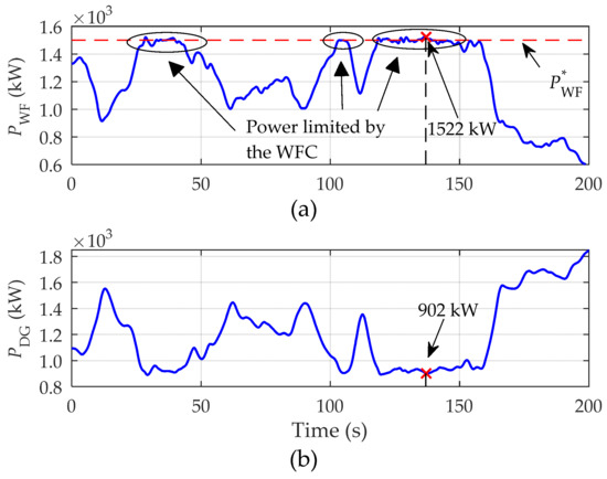
Figure 10.
Delivered active power: (a) Wind farm; (b) Diesel power plant.
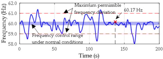
Figure 11.
Time domain behavior of grid frequency.
2.4. Analysis of the Results and Problem Statement
The time domain behavior of the output power delivered by the wind turbine shown in Figure 10a reveals a correct performance in power curtailment around the predefined set point, P*WF = 1500 kW. When the available active power is below the set point value, the wind energy is dispatched according to the optimal wind power conversion criterion, as expected. Complementarily, in Figure 10b, it can be seen that the fluctuating wind power injection is effectively absorbed by diesel generators in order to match the power generation and consumption. It should be noted the similarity between the values highlighted in Figure 10 and those provided in Table 3. This fact allows to validate the implemented SCHPS-model in terms of accuracy.
In reference to Figure 11, the grid frequency presents an inadmissible evolution in terms of power quality. This figure shows the permissible frequency ranges established by the Ecuadorian Grid Code (EGC) [25], which are mandatory for any generation unit integrated to the National Bulk Power System. The EGC requires that the nominal frequency be set to 60 Hz, with a control range of ± 0.15 Hz (under normal conditions). In order to avoid unnecessary trip of frequency relays, the EGC recommends to maintain the grid frequency excursion between the values 59–61 Hz. However, since the particular characteristics of the SCHPS (isolated operation, small-capacity of synchronous generators, high wind energy penetration levels, and others) make the frequency control tasks difficult, some solutions aimed at improving the power quality indexes have to be proposed. These solutions are discussed in the following sections and are applied to both the diesel power plant and the wind farm.
3. Proposals to Enhance the Power System Frequency Control under Normal Conditions
In this section, some proposals intended to enhance frequency control actions in a weak and isolated power system with high wind energy penetration are presented. These solutions consider the adjustment of certain parameters of the diesel-engine speed governors and the incorporation of additional control strategies to the wind turbine controllers.
3.1. Adjustment of the Control Gains of the Diesel-Engine Speed Governor
The first improvement proposal, and the only one applied to the conventional power plant, consists of readjusting the controller gains associated to each diesel-engine speed governor (Figure 2) based on a stability analysis. By considering identical characteristics of the diesel generator units and their speed governors (a real situation in the SCHPS), it is possible to obtain an aggregate representation of the thermal power plant and incorporate it in the LFC-scheme as shown Figure 12. In this scheme, wT denotes the equivalent energy share factor that, in this case, can be calculated as a sum of the individual energy share weights, wi (see the definition of wi in Section 2.1.)
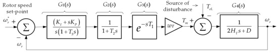
Figure 12.
Aggregate representation of the diesel power plant in the LFC-scheme.
The linear system schematized above corresponds to an alternative representation of the LFC-scheme shown in Figure 1b, which is derived by considering the torque difference in the swing Equation (1) instead of small power deviations, as it is expressed in (4). In this equation, Tm and TeL are the mechanical and the electromagnetic-load torque expressed in per unit. Since the variable-speed wind turbine lacks a natural response to the grid frequency deviations, its model is not considered in the stability analysis presented in this section. However, its potential contribution to the grid frequency support will be studied in detail in Section 3.3.
In order to evaluate the disturbance rejection ability of the speed governor while maintaining the rotor speed around its set-point (nominal grid frequency), the closed-loop transfer function that relates the output variable, ωr, and the input variable, TeL, in Figure 12, can be formulated as (5). The transfer functions G1(s)–G4(s) are graphically defined in this figure.
For obtaining a rational transfer function form from (5), the time-delay characteristic introduced by G3(s) is approximated by using the first-order Páde approximant [26], as follows:
By substituting (6) in (5), the following symbolic equation is attained:
For a numerical evaluation of the previous equation, the real case of study depicted in Section 2.1. will be considered (where: HT = 2 × 0.4208 s, D = 0.5, and wT = 2/3, and the information summarized in the Appendix). The resulting expression is:
Now, the stability margin of the SCHPS is determined by analyzing the trajectory described by the eigenvalues on the s-plane as a consequence of a gradual increase of a system gain, K. According to the classical control theory, such gain is introduced in the characteristic equation as follows:
Note in (9) that, for the particular linear system studied in this work, the K gain affects to the entire set of parameters of the speed governor as well as the inertial characteristics of the power system. Given the difficulty of modifying the value of some intrinsic parameters of the LFC-scheme (such as time constants, constant of inertia and damping effects), the only parameters that can be adjusted to produce a change in K are the control gains of the speed governor of the diesel generator: KP and KI.
Figure 13 shows the root-locus plot generated from (8). It reveals that the SCHPS is stable when K = 1 (that is, by using the default values of the controller gains specified in the Appendix) and it will remain under this condition as long as the gain K is less than 33.6. This critical value gives the maximum multiplying factor of the controller gains, KP and KI, that ensures a stable response of the system under contingency and guarantees a proper load sharing in normal operating conditions.
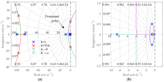
Figure 13.
Root-locus stability analysis of the SCHPS: (a) All poles; (b) Detailed zone of dominant poles.
Complementarily, Figure 14 shows the effect of increasing K on the dynamics of the frequency of the SCHPS model implemented in MATLAB/Simulink®. As expected, larger values of K improve the frequency recovery process in terms of the maximum instantaneous frequency deviation (absolute peak value), the recovery time, and the settling time. However, increasing values of K give place to complex conjugated poles (See dominant poles trajectory in Figure 13b), and an oscillation will appear after the frequency rebound, the higher value of K, the more sustained the oscillation. When K reaches its critical value, the power system becomes unstable.
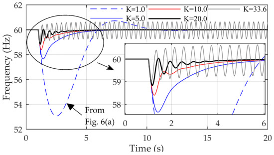
Figure 14.
Effect of increasing K on the frequency recovery process of the SCHPS.
From the results presented in Figure 14, it can be concluded that there is a specific margin for increasing the K gain that could enhance the frequency response of the power system in amplitude and time. However, due to the subjectivity of the term “most suitable” to define the desired frequency response, the selection of the multiplying factor K has to be made by using a purely technical criterion based on three specific objectives: (1) attain a faster response from the controller in the frequency recovery process; (2) reduce the frequency drop and; (3) after the frequency rebound, damp the remaining frequency oscillations in a relative short time. Objectives 1 and 2 are designed to maintain an adequate power quality index and the latter is aimed to avoid causing additional mechanical stress in the diesel engine drives during the frequency control process. In this work, it has been verified that a factor of multiplication of K = 10 allows to fulfill the objectives described before. Figure 15 shows the results obtained by adjusting the diesel-engine controller gains and applying such modifications to the SCHPS model implementation particularized to the case of study presented in Section 2.3. In this figure, it can be seen that the power delivered by diesel generators improves the absorption of the fluctuating wind power injection in order to match the generated and demanded power in the power system. As a consequence, the excursions of the frequency are appreciably reduced, being great part of these within the band of control required by the applicable grid code. Similar benefits can be observed in the evolution of the rate of change of frequency (ROCOF). With the implementation of the corrective actions on the conventional generation, the average value of this variable is reduced by approximately 89%, which leads to substantially reduce the risk of triggering of frequency relays installed at different points in the SCHPS.
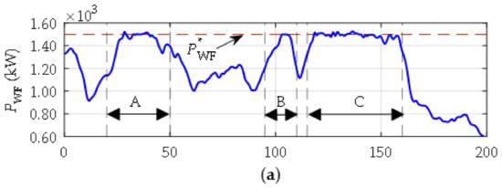
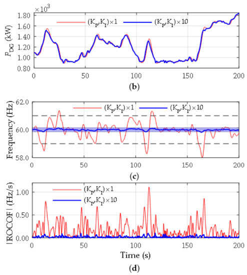
Figure 15.
Adjustment of the control gains of the diesel-engine speed governor and its effect on the power system dynamics: (a) Wind farm generated power; (b) Diesel power plant production; (c) Grid frequency and; (d) ROCOF.
3.2. Improvement of the Wind Power Curtailment Strategy
The wind power curtailment strategy implemented in the SCHPS, and presented in Section 2.2., acts directly on the blade pitch angle to limit the power delivered by each wind turbine to a maximum value established by the centralized wind farm control, WFC. Although the results obtained in the simulation reveal that these control actions are performed properly, the handling of mechanical variables might introduce transient errors in the set-point tracking Pset, inducing small grid frequency deviations as a consequence of the non-continuous wind power injection under curtailment operation mode (Figure 10a and Figure 11). At first glance, it would seem that an increase of the gains of the PI controller implemented in the WTC (Figure 7b) could improve the effectiveness of the existing control strategy. However, it is not a suitable solution since it would subject the turbine blades to an additional mechanical stress caused by greater variations of the pitch angle for wind power limitation. The control strategy proposed in this section aims to improve the performance of the control philosophy implemented in the real wind farm and is based on the idea of combining the use of electromagnetic and mechanical variables for wind power curtailment.
The method consists of modifying the MPPT curve, implemented in the wind turbine speed controller, by adjusting the upper limit of the active power to be generated, Pmax, to the curtailment level required by the WFC, Pset, as illustrated in Figure 16a. If the incoming wind speed causes the mechanical power transmitted to the shaft to be below Pset, the wind turbine will dispatch its active power under the default optimal conversion criterion. On the contrary, if the mechanical power delivered by the turbine exceeds Pset, the wind turbine will inject at most the set-point power Pset. Since, in this situation, the inner wind turbine power mismatch would cause an undesirable rotor over-speeding, it is necessary to compensate such imbalance by acting on the blade pitch control system. In order to address this, a new maximum rotor speed reference, ω’max, has to be specified. A new operating zone (points C’ and D’ in Figure 16b) is defined by displacing the quasi-constant speed zone of the MPPT curve along the optimal power locus until its maximum power value coincides with the specified Pset. Such operating zone is characterized by the power values Pset and P1, and the rotor speeds ω’1 and ω’max.
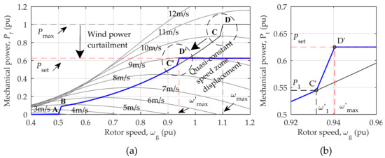
Figure 16.
Active power curtailment procedure: (a) MPPT curve clipping; (b) Quasi-constant speed zone under curtailed condition.
The displacement of the quasi-constant speed zone is achieved by substituting the values Pset, P1, ω’1 and ω’max, by Pmax, Pv(base), ω1 and ωmax, in Equation (3), respectively. The values associated to the new operating points, C’ and D’, can be calculated by considering the same power and speed ratios than in the quasi-constant speed zone of the default MPPT curve, as follows:
Since point C’ is still located in the optimization zone, ω’1 can be calculated by using (3) as follows:
Figure 17 shows the schematic implementation of the proposed strategy in the wind turbine. The values Pset, P1, ω’1 and ω’max, are applied to the WTC, in order to evaluate the MPPT curve and, ω’max to the blade pitch angle controller for a proper rotor speed limitation. Since the proposal is designed to be implemented locally in the WTC associated with the i-th wind turbine, the external configuration of the wind farm controller will maintain its original topology (Figure 7a).
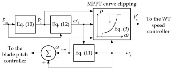
Figure 17.
Implementation of the wind power curtailment proposal on the i-th WTC.
Figure 18 and Figure 19 show the results obtained by implementing the proposal in the SCHPS model for the case of study described in the final part of previous subsection (with the diesel-engine speed governor gains readjusted). These results are compared with those generated by considering the original wind farm controller (blue line curves in Figure 15). In order to better show the time evolution of the variables of interest, only those intervals where the wind power is curtailed (defined as A, B, and C in Figure 15a) are shown in Figure 18. This is because outside these temporal ranges, the dynamics obtained in the two cases compared are practically the same.
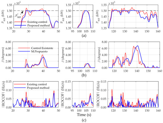
Figure 18.
Time-domain simulation results by implementing the wind curtailment proposal: (a) Wind farm output power; (b) Blade pitch angle and; (c) ROCOF.
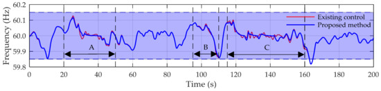
Figure 19.
Effects of the proposal on the grid frequency.
In Figure 18a, it can be seen the notorious improvement in the wind curtailment performance achieved with the proposed method, as expected. Since the control strategy is based on a combined action of electromagnetic and mechanical variables to perform a finer tracking of the set-point signal Pset, the evolution of the blade pitch angle is much smoother as it can be seen in Figure 18b. Regarding the ROCOF, the implementation of the proposal allows to achieve an average reduction of this variable by 21.66% as shown in Figure 18c. Finally, Figure 19 shows the reduction of frequency fluctuations obtained by applying the proposal, specifically in those intervals corresponding to the actions of wind power curtailment. In order to better show the grid frequency excursions in this figure, the scale of the y-axis has been adjusted around the control frequency range specified by the grid-code described in Section 2.4., and it will be kept that way for depicting the rest of results.
3.3. Inertial Control Strategy Applied to the Wind Turbines
This section presents a third improvement proposal aimed to reduce the fluctuating wind power injection to the grid under normal operating conditions and, to provide grid frequency support in case of contingency. The inertial control strategy presented below is based on [12] and has been named Extended Optimal Power Point Tracking (EOPPT). It has been designed to be implemented in the speed controller of the wind turbine (Figure 3) and its principle of operation is based on the extraction of kinetic energy stored in the rotating masses to produce controlled variations of the output active power depending on two input variables: the deviation of the grid frequency, Δf, and the time derivative of frequency, df/dt. Unless this kind of control strategy is implemented, a full converter based wind turbine would not be able to reveal its inertial resources to the grid in a natural manner, because the DC-link decouples the frequencies of both sides of the converter (MSC and GSC), so that frequency variations in the grid do not reflect in frequency variations in the electrical generator terminals. To briefly explain the mechanics of the method, let us assume that the wind turbine is operating at point A in Figure 20 under a fixed wind speed condition. In case the power system experiences an under-frequency event, the wind turbine is required to increase its active power injection to the grid. This action can be done by moving the operation point to B immediately by means of a controlled shifting of the MPPT curve to the left. At this operating point, the imbalance between the mechanical power developed by the turbine and the electrical power required by the generator causes the rotor angular deceleration until a new equilibrium condition is reached at point C. Through the path A→B→C, the wind turbine will have to deliver part of its kinetic energy to provide frequency support to the grid. After that, the method will force the wind turbine to recover its pre-disturbance operating point, A. On the contrary, if an over-frequency event takes place, the active power set-point applied to the speed controller of the wind turbine will have to follow the path A→D→E→A.
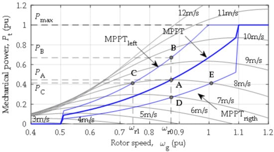
Figure 20.
MPPT curve shifting procedure.
Figure 21 shows the general scheme for the implementation of the EOPPT-method in the wind turbine. This scheme is made up of two subsystems: the frequency deviation dependent loop and the time derivative of frequency loop. The first loop receives the rotor speed, ωg, and the deviation of the grid frequency, Δf, as input variables. The latter variable is passed through a first-order low pass filter (with time constant, Two) in order to remove the steady-state error of the grid frequency introduced by the primary frequency regulation tasks. The control actions provided by this subsystem are driven by (13), which has been derived in [12]. In this equation, fKopt, is the virtual inertia factor, ωr0 is the pre-disturbance rotor speed, kvir is the virtual inertia coefficient, Δf’ is the filtered frequency deviation, and p is the number of pole pairs of the electrical generator. The shifting of the MPPT curve, either to the left or to the right, is achieved by multiplying fKopt by the optimization constant Kopt in (3). CTRL is a binary control signal that is activated whenever a non-zero frequency deviation is detected, which is necessary for allowing a continuous updating of ωr0. Finally, in order to restrict the shifting of the MPPT curve within safe and stable operating ranges, the limits fKopt,max and fKopt,min, have been included in the control scheme.
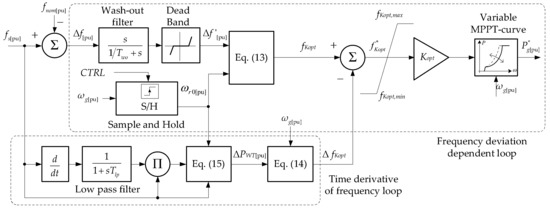
Figure 21.
Extended Optimal Power Point Tracking method scheme.
On the other hand, the time derivative of frequency loop is conceived to provide a complementary frequency support and is focused on the reduction of the ROCOF. The control actions resulting from this subsystem are given by (14), which have been also derived in [12], where: Δfkopt is the virtual inertia factor deviation, fs is the measurement of the grid frequency (fs[pu] = ωs[pu]), Heq is the equivalent constant of inertia of the wind turbine, ωmax and ωmin are the rotor speed limits, graphically defined in Figure 4, and Tlp is the time constant of the low pass filter designed to eliminate the measurement noise. The values assigned to the parameters of the EOPPT-method are summarized in Appendix A.
where:
Figure 22 depicts the dynamics obtained by implementing the EOPPT-method in the wind turbines WT1, WT2 and WT3 under operating conditions similar to those presented in Section 3.2. Note in Figure 22a that the generated wind power is slightly smoothed in those intervals outside the power curtailment condition. This produces a noticeably reduction of the ROCOF (Figure 22b), whose average value decreases in an additional 15% compared to the results achieved in the previous subsection. In addition, the application of the EOPPT-method in the wind turbines allows a milder evolution of the grid frequency as shown in Figure 22c.
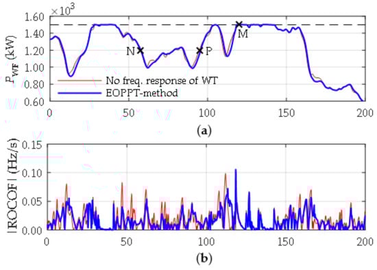
Figure 22.
Time domain simulation with the application of the EOPPT-method: (a) Dispatched wind power; (b) ROCOF and; (c) Grid frequency.
4. Assessment of the Improvement Proposals under Contingency Conditions
The proposals aimed to improve the frequency control actions of the SCHPS, in the previous section, have been discussed and tested by considering normal operating conditions, characterized by a fluctuating behavior of the grid frequency due to the injection of a realistic wind power profile. Although the previous results reveal a significant reduction of frequency deviation and an important decrease of the average ROCOF by applying these solutions, it is essential to consider more severe operating scenarios in which the loss of generation or demand may involve a risk to the power supply continuity. The most probable scenario for the occurrence of a contingency in the actual power system corresponds to the sudden loss of wind generation, a fact that will be considered in the following study. For the test power system, similar operating conditions to those described in Section 3.3. are taken into account, and a new base case is defined. It considers all the improvement proposals introduced throughout the previous section, except the EOPPT-method (red line curves in Figure 22). The disturbance is generated by disconnecting the wind turbine WT3 (Figure 1) at three different instants within the time frame considered in the simulations: points P, N, and M, which have been highlighted in Figure 22a. These points correspond to three operational status of the wind farm that are interesting for the assessment of the EOPPT-method under contingency conditions:
- Case P: Tripping of WT3 when the incoming wind speed is increasing (dv/dt > 0)
- Case N: Tripping of WT3 when the incoming wind speed is decreasing (dv/dt < 0)
- Case M: Tripping of WT3 under highly favorable wind conditions (Curtailment)
Figure 23 summarizes the results obtained by simulating each case of study.The performance of the power system for the first contingency scenario (Case P) is depicted in Figure 23a. The upper subfigure illustrates the time-domain behavior of the power delivered by each machine installed in the wind farm along with the maximum output power set-point imposed by the wind farm controller, Pset. Note that, at the moment of the disconnection of WT3, the value of Pset increases from 500 to 750 kW. This is because the wind farm output power reference P*WF (Computed as 1500 kW in Section 2.3.) has to be fulfilled only by the remaining two online wind turbines. Since a non-variable load demand profile is considered in the simulation, the value of P*WF will remain unchanged throughout the simulated time frame. The subsequent subfigures show the dynamics of the power dispatched by the wind farm, the behavior of the power delivered by the diesel power plant, the response of the grid frequency, and the evolution of the ROCOF. These illustrations reveal that a sudden loss of wind power of 400 kW causes a grid frequency drop which is effectively mitigated by the wind turbines by implementing the EOPPT-method: the maximum instantaneous frequency deviation (MIFD) is reduced in 42.88% in comparison with the base case. The inertial response from wind turbines helps to the conventional generation in the frequency controls tasks, a fact that can be seen in the diesel power generation subplot, where a milder dynamic of the mechanical power is achieved. Since the increase of active power required for frequency support is backed up by an increase in the available mechanical power, due to dv/dt > 0, a reduction of the maximum rate of change of frequency, |ROCOF|max, is achieved.
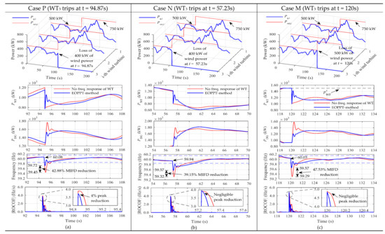
Figure 23.
Power system response under different contingency scenarios: (a) Case P; (b) Case N and (c) Case M.
For the case N (Figure 23b), similar conclusions can be drawn: the wind turbines contribute to the reduction of the MIFD in 39.15% and facilitate the frequency regulation performed by synchronous generation. However, in this particular situation, where dv/dt < 0, the kinetic energy stored in the wind turbine will be spent faster during the frequency support stage which leads to have a minimum effect on the reduction of |ROCOF|max. In the third case, the contingency occurs when the wind turbines are operating under curtailment conditions (Figure 23c). According to the curtailment philosophy discussed in Section 3.2., the wind turbine will be operating at power and rotor speed maximum conditions, Pset and ω’max, and, unless these values undergo a change imposed by the WFC, the wind turbine will not be able to provide frequency support to the grid. Nevertheless, as it has been explained before, the disconnection of one wind turbine forces the others to cover the missed power by increasing the individual reference signal Pset until the total wind farm power reaches its set-point value, P*WF. This enables the online wind turbines to play an important role in the frequency recovery process, attaining a significant reduction of MIFD of 47.53% and a slightly improvement of |ROCOF|max.
5. Conclusions
This paper presents some proposals aimed at enhancing frequency control actions in a weak and isolated power system with an important penetration of wind energy. As a case of study, the San Cristobal hybrid power system (Galapagos Islands-Ecuador) has been considered, whose time-domain behavior has been studied by using the Load Frequency Control approach described in the first part of this work. The implemented model has been validated after recreating certain actual operative situations of the power system and comparing the results with the available records acquired in field tests. The preliminary results show the technical challenge experienced by this type of systems in the frequency control tasks, specifically under scenarios characterized by high share of intermittent wind energy in the power demand covering. This results in prominent frequency fluctuations under normal operating conditions, which might cause under/over frequency relays tripping at different points of the power system, putting at risk the power supply continuity.
A first action intended to solve this problem, consists of a procedure to quantify the stability margin of the power system, whose frequency control is completely governed by the conventional synchronous generation. It has been found that a readjustment of the speed governor gains, by respecting the stability margin previously computed, allows to substantially improve the frequency quality indicators. The final selection of the controller gains has been done by applying a purely technical approach based on three objectives: fast frequency recovery, frequency drop reduction, and frequency rebound stage with small oscillations. However, better results could be obtained if an optimization process for tuning the controller gains is performed. Unfortunately, the applicable grid code does not provide enough criteria for defining an objective function (according to the objectives described above) and even for the constraints of the optimization problem, so, further studies on this topic is recommended as future work.
Another two improvement proposals are devised to be implemented in the wind turbine, as causing agent of the main issue addressed in this work. In this sense, a second corrective action, which constitutes the main contribution of this paper, consists in proposing an improved wind power curtailment strategy. This strategy combines the use of electromagnetic and mechanical variables to carry out such limitation in a more effective way, in response to the requirements established by the wind farm controller, either for technical or environmental reasons. As positive aspects of the implementation of this proposal, the results obtained by simulation show that the injection of a practically constant wind power under highly favorable wind conditions considerably reduces the associated frequency fluctuations, providing an additional margin of improvement in this regard. Also, the proposal produces a smaller and milder variation of the pitch angle during the power limitation, which could positively impact to the wear and tear of the wind turbine due to the reduction of the mechanical stress exerted on the blades. Nevertheless, it must be kept in mind that the actual effects of the proposal on the wind turbine aging can be only evaluated by long-term field research on real prototypes, therefore, a specialized study in this regard is suggested.
In addition, in order to cover those intervals where the wind energy is dispatched under the criterion of optimal conversion (non-curtailment condition), the implementation of an inertial control based strategy is presented as a third corrective action. Such strategy is designed to be incorporated in the wind turbine controllers to enable its participation in the grid frequency support tasks in cooperation with the conventional synchronous generation. After subjecting the test system to normal operating conditions and to contingency situations, it was found that this solution allows to enhance the overall performance of the system during the frequency recovery stage. This improvement would allow the system operator to define less restrictive wind power curtailment levels for a greater participation of the wind power in the electrical demand covering without compromising the security of the power system. This would lead to a smaller wind energy waste while increasing the economic and ecological benefits derived from electrical exploitation in the San Cristobal Island.
Acknowledgments
This work was supported by the Secretaria de Educacion Superior, Ciencia, Tecnologia e Innovacion (SENESCYT), Government of the Republic of Ecuador (grant number: 2015-AR6C5141). The authors would like to thank the companies ELECGALAPAGOS S.A. and EOLICSA for providing information regarding the operation and control of the San Cristobal power system (Galapagos Islands-Ecuador).
Author Contributions
Danny Ochoa conceived and designed the paper; Danny Ochoa carried out the time-domain simulations; Danny Ochoa and Sergio Martinez analyzed the results and wrote the paper; Sergio Martinez guided the whole work and the direction of the research.
Conflicts of Interest
The authors declare no conflict of interest.
Appendix A
- A.
- Diesel-engine speed governor parameters: T1 = 0.024 s, T2 = 0.1 s, T3 = 0.01 s, Tmax = 1.1 pu, Tmin = 0 pu, KP = 2.294, KI = 1.458.
- B.
- Variable-speed wind turbine parameters:
Table A1.
Wind turbine parameters.
Table A1.
Wind turbine parameters.
| Parameter | Symbol | Value |
|---|---|---|
| Rated power (base power) | Pbase | 800 kW |
| Max./Min. active power | Pg,max/Pg,min | 1/0.04 pu |
| Max./Min. electromagnetic torque | Tem.max/Tem.min | 0.91/0.08 pu |
| Base wind speed | vbase | 10 m/s |
| Active power at vbase | Pv(base) | 697 kW |
| Generator pole pairs number | p | 2 |
| Generator nominal frequency | fg,nom | 50 Hz |
| Base speed of the turbine | ωt,base | 2.37 rad/s |
| Base speed of the generator | ωg,base | 157.08 rad/s |
| Gearbox speed ratio | nt | 66.185 |
| Air density | ρ | 1.225 kg/m3 |
| Radius of the rotor | R | 29.5 m |
| Equivalent constant of inertia | Heq | 4.18 s |
| Optimization constant | Kopt | 0.6728 |
| Min./Max. blade pitch angle | βmin/βmax | 0/88° |
| Maximum blade pitch angle rate | (dβ/dt)max | 10°/s |
| Generator and converter time constant | τC | 20 ms |
| Blade pitch servo time constant | τP | 0.3 s |
| Pitch controller gains | KPpc/KIpc | 150/25 |
| Speed controller gains | KPsc/KIsc | 0.3/8 |
- C.
- MPPT curve parameters: ωmin = 0.5 pu, ω0 = 0.51 pu, ω1 = 1.09 pu, ωmax = 1.1 pu.Power coefficient equation [27]:where:
- D.
- E.
- Extended OPPT method parameters: Dead band = 1 mHz, kvir = 4, fKopt,max = 1.6, fKopt,min = 0.4, Two = 10 s, Tlp = 0.8 s.
References
- Lu, J.; Wang, W.; Zhang, Y.; Cheng, S. Multi-Objective Optimal Design of Stand-Alone Hybrid Energy System Using Entropy Weight Method Based on HOMER. Energies 2017, 10, 1664. [Google Scholar] [CrossRef]
- Martínez-Lucas, G.; Sarasúa, J.; Sánchez-Fernández, J. Frequency Regulation of a Hybrid Wind–Hydro Power Plant in an Isolated Power System. Energies 2018, 11, 239. [Google Scholar] [CrossRef]
- Kies, A.; Schyska, B.; von Bremen, L. Curtailment in a Highly Renewable Power System and Its Effect on Capacity Factors. Energies 2016, 9, 510. [Google Scholar] [CrossRef]
- Bird, L.; Lew, D.; Milligan, M.; Carlini, E.M.; Estanqueiro, A.; Flynn, D.; Gomez-Lazaro, E.; Holttinen, H.; Menemenlis, N.; Orths, A.; et al. Wind and solar energy curtailment: A review of international experience. Renew. Sustain. Energy Rev. 2016, 65, 577–586. [Google Scholar] [CrossRef]
- Al-Sarray, M.; McCann, R.A. Control of an SSSC for oscillation damping of power systems with wind turbine generators. In Proceedings of the 2017 IEEE Power Energy Society Innovative Smart Grid Technologies Conference (ISGT), Washington, DC, USA, 23–26 April 2017; pp. 1–5. [Google Scholar]
- Kim, C.; Muljadi, E.; Chung, C. Coordinated Control of Wind Turbine and Energy Storage System for Reducing Wind Power Fluctuation. Energies 2017, 11, 52. [Google Scholar] [CrossRef]
- Dou, X.; Quan, X.; Wu, Z.; Hu, M.; Sun, J.; Yang, K.; Xu, M. Improved Control Strategy for Microgrid Ultracapacitor Energy Storage Systems. Energies 2014, 7, 8095–8115. [Google Scholar] [CrossRef]
- Diaz-Gonzalez, F.; Bianchi, F.D.; Sumper, A.; Gomis-Bellmunt, O. Control of a Flywheel Energy Storage System for Power Smoothing in Wind Power Plants. IEEE Trans. Energy Convers. 2014, 29, 204–214. [Google Scholar] [CrossRef]
- Lotfy, M.E.; Senjyu, T.; Farahat, M.A.-F.; Abdel-Gawad, A.F.; Yona, A. A Frequency Control Approach for Hybrid Power System Using Multi-Objective Optimization. Energies 2017, 10, 80. [Google Scholar] [CrossRef]
- Ren, G.; Liu, J.; Wan, J.; Guo, Y.; Yu, D. Overview of wind power intermittency: Impacts, measurements, and mitigation solutions. Appl. Energy 2017, 204, 47–65. [Google Scholar] [CrossRef]
- Ma, H.; Wang, B.; Gao, W.; Liu, D.; Sun, Y.; Liu, Z. Optimal Scheduling of an Regional Integrated Energy System with Energy Storage Systems for Service Regulation. Energies 2018, 11, 195. [Google Scholar] [CrossRef]
- Ochoa, D.; Martinez, S. Fast-Frequency Response Provided by DFIG-Wind Turbines and its Impact on the Grid. IEEE Trans. Power Syst. 2017, 32, 4002–4011. [Google Scholar] [CrossRef]
- Naik, K.A.; Gupta, C.P. Output Power Smoothing and Voltage Regulation of a Fixed Speed Wind Generator in the Partial Load Region Using STATCOM and a Pitch Angle Controller. Energies 2017, 11, 58. [Google Scholar] [CrossRef]
- Kerdphol, T.; Rahman, F.S.; Mitani, Y.; Hongesombut, K.; Küfeoğlu, S. Virtual Inertia Control-Based Model Predictive Control for Microgrid Frequency Stabilization Considering High Renewable Energy Integration. Sustainability 2017, 9, 773. [Google Scholar] [CrossRef]
- Lee, H.; Hwang, M.; Muljadi, E.; Sørensen, P.; Kang, Y.C. Power-Smoothing Scheme of a DFIG Using the Adaptive Gain Depending on the Rotor Speed and Frequency Deviation. Energies 2017, 10, 555. [Google Scholar] [CrossRef]
- Ma, S.; Geng, H.; Yang, G.; Pal, B.C. Clustering based Coordinated Control of Large Scale Wind Farm for Power System Frequency Support. IEEE Trans. Sustain. Energy 2018, 1. [Google Scholar] [CrossRef]
- Raoofsheibani, D.; Abbasi, E.; Pfeiffer, K. Provision of primary control reserve by DFIG-based wind farms in compliance with ENTSO-E frequency grid codes. In Proceedings of the IEEE PES Innovative Smart Grid Technologies, Istanbul, Turkey, 12–15 October 2014; pp. 1–6. [Google Scholar]
- Bignucolo, F.; Cerretti, A.; Coppo, M.; Savio, A.; Turri, R. Effects of Energy Storage Systems Grid Code Requirements on Interface Protection Performances in Low Voltage Networks. Energies 2017, 10, 387. [Google Scholar] [CrossRef]
- Yuan, C.; Xie, P.; Yang, D.; Xiao, X. Transient Stability Analysis of Islanded AC Microgrids with a Significant Share of Virtual Synchronous Generators. Energies 2018, 11, 44. [Google Scholar] [CrossRef]
- Theubou, T.; Wamkeue, R.; Kamwa, I. Dynamic model of diesel generator set for hybrid wind-diesel small grids applications. In Proceedings of the 2012 25th IEEE Canadian Conference on Electrical Computer Engineering (CCECE), Montreal, QC, Canada, 29 April–2 May 2012; pp. 1–4. [Google Scholar]
- Yoo, J.I.; Kim, J.; Park, J.W. Converter control of PMSG wind turbine system for inertia-free stand-alone microgrid. In Proceedings of the 2016 IEEE Industry Applications Society Annual Meeting, Portland, OR, USA, 2–6 October 2016; pp. 1–8. [Google Scholar]
- Gonzalez-Longatt, F.; Bonfiglio, A.; Procopio, R.; Bogdanov, D. Practical limit of synthetic inertia in full converter wind turbine generators: Simulation approach. In Proceedings of the 2016 19th International Symposium on Electrical Apparatus and Technologies (SIELA), Bourgas, Bulgaria, 29 May–1 June 2016; pp. 1–5. [Google Scholar]
- Ochoa, D.; Martinez, S. A Simplified Electro-Mechanical Model of a DFIG-based Wind Turbine for Primary Frequency Control Studies. IEEE Lat. Am. Trans. 2016, 14, 3614–3620. [Google Scholar] [CrossRef]
- Proyecto Eólico Isla San Cristóbal—Galápagos 2003–2016. Available online: https://www.globalelectricity.org/content/uploads/Galapagos-Report-2016-Spanish.pdf (accessed on 11 April 2018).
- Agencia de Regulación y Control de Electricidad. Procedimientos de Despacho y Operación. Available online: http://www.regulacionelectrica.gob.ec/wp-content/uploads/downloads/2015/10/ProcedimientosDespacho.pdf (accessed on 13 February 2018).
- Natori, K. A design method of time-delay systems with communication disturbance observer by using Pade approximation. In Proceedings of the 2012 12th IEEE International Workshop on Advanced Motion Control (AMC), Sarajevo, Bosnia and Herzegovina, 25–27 March 2012; pp. 1–6. [Google Scholar]
- Junior, C.R.S.; Lima, F.K.A. Wind Turbine and PMSG Dynamic Modelling in PSIM. IEEE Lat. Am. Trans. 2016, 14, 4115–4120. [Google Scholar] [CrossRef]
© 2018 by the authors. Licensee MDPI, Basel, Switzerland. This article is an open access article distributed under the terms and conditions of the Creative Commons Attribution (CC BY) license (http://creativecommons.org/licenses/by/4.0/).