HIL Co-Simulation of Finite Set-Model Predictive Control Using FPGA for a Three-Phase VSI System

Abstract

The conversion and control for the utilization of power generated from energy sources can be performed using a power electronic converter system. The voltage source inverter (VSI) is one of the commonly used converter topologies, being controlled by a switching control algorithm for power conversion. Finite set-model predictive control (FS-MPC) is a modern switching control algorithm and has received significant attention due to its predictive nature. In this paper, the implementation of FS-MPC is presented for the load-side current control of a three-phase VSI system using an integrated platform of MATLAB/Simulink and Xilinx system generator (XSG). The XSG provides the functionality of digital design and intuitive implementation of field-programmable gate array (FPGA) controlled systems. The additional functionality of hardware-in-the-loop (HIL) co-simulation using FPGA is used for the testing and validation of controller performance. The controller performance is validated through three platforms: MATLAB/Simulink, XSG and HIL co-simulation using ZedBoard Zynq evaluation and development FPGA kit.

1. Introduction

In recent years, the energy demand has been growing at a rapid rate and causing major global concern related to the depletion of nonrenewable energy sources and global warming due to environmental pollution. Accordingly, to fulfill the rise in energy demands and reduce the use of nonrenewable energy sources, energy from renewable sources is required to be generated more and more in the future for clean and green energy without affecting the environment [1,2,3]. Solar energy and wind energy are the prominent renewable sources to generate power. However, power conversion and control is required to use the generated power from solar and wind efficiently. Voltage source inverter (VSI) power topology has been widely utilized for the controlled and efficient conversion of electrical power. The applications of VSI systems include industrial drives, active filters, high power factor ac-dc converters, vehicular systems, uninterruptible power supplies (UPS), and the grid connection of renewable energy systems [4,5,6]. The design of a suitable controller is essential for the efficient and controlled conversion of electrical power. Different current control techniques have been employed for three-phase VSI systems and studied extensively in the last decades.

The current control methods that have been developed for the VSI system can be categorized as conventional and modern controllers/linear and nonlinear controllers. The conventional linear controllers such as pulse width modulation (PWM) and space vector modulation (SVM) require carrier-based modulators. Nonlinear controllers such as hysteresis current controllers (HCC), which are based on comparators, require high switching frequency for effective operation. The conventional linear and nonlinear controllers have been widely studied and developed for the three-phase VSI system applications [7,8,9]. In addition to these conventional control techniques, advanced controllers are also employed to improve the performance of the VSI system. However, the increased complexity and computational burden of the advanced controllers are the prime concern for their implementation.

The model predictive control (MPC) technique is one of the advanced controllers employed for power converters because of their advantages as compared to the conventional controllers, such as better dynamic performance, handling of multi-input multi-output (MIMO) cases, and flexibility for the inclusion of constraints and nonlinearities [10,11,12,13]. The intuitive design of the controller based on the predictive model and cost function-based selection of the optimized switching state are additional features of MPC. MPC strategies are broadly classified as continuous set-MPC (CS-MPC) and finite set-MPC (FS-MPC) [14]. The CS-MPC computes continuous control signals with constant switching frequency by using a modulator, whereas FS-MPC implements the MPC algorithm by utilizing the discrete nature of the power converter and applies the switching signals directly to the power converter without the need for an external modulator. FS-MPC is designed to reduce the computational burden of the algorithm by utilizing the set of possible switching states of power converters for solving the optimization problem online.

MPC has been proven as a mature strategy for power converters and drives applications such as three-phase neutral-point-clamped systems [15,16], active front-end rectifiers [13,17], cascaded H-bridge converters [18,19], flying capacitor converters [16,20], and matrix converters [13,21]. The practical implementations of MPC for power converters are mainly based on software-based control using a microprocessor/digital signal processor (DSP) [13,22,23,24,25,26]. These micro-programmable solutions have advantages such as simple circuitry, software-based control, and flexible control adaptability to different applications. However, these have some disadvantages, such as delay in the computation of the optimized switching state. This delay problem has been clearly recognized and some modifications have been given for its compensation [13,22]. In addition, they require a high processing power for the implementation of complex controllers.

Considering the above mentioned limitations, the field-programmable gate array (FPGA) represents an effective alternative because of its parallel processing environment for practical implementation [27,28]. FPGA is considered as the better option for controller designing and prototyping due to its characteristics of configurability and programmability [29,30]. However, real-time controller implementation using FPGA has been found to be difficult and requires specialized training in the hardware description language (HDL). Therefore, prototype designing is a complex and time-consuming task, even for skilled researchers or engineers, with an increasing level of complexity [29,31].

The Xilinx system generator (XSG) platform provides a virtual FPGA environment for the designing, testing, and development of digital controllers. The integrated platform of MATLAB/Simulink-XSG provides the functionality of automatic HDL code generation that can be further utilized for the straightforward implementation of FPGA-based experimental system prototypes without the additional knowledge of HDL [32,33,34]. XSG provides a modelling-based design approach for digital system implementation. Therefore, XSG-based system modelling is required for the development of real-time systems using FPGA through automatic HDL code generation. Further, the recent availability of a model-based FPGA design platform integrated with MATLAB/Simulink provides the functionality of hardware-in-the-loop (HIL) co-simulation.

The HIL co-simulation is a way to test the controller by including actual hardware and moving a step forward towards the realism of the software-based simulated system. The software-based simulation of a plant system or control system can be substituted using actual hardware to perform HIL co-simulation by interacting with a computer. HIL co-simulation can be used as a platform to validate the controller using the actual hardware by interacting with the plant system simulated by the computer. In addition, the platform can be used for the development of novel control strategies without using an actual plant system that can be damaged during the testing of controller.

This paper proposes a novel implementation of the FS-MPC through modelling in an XSG environment integrated with MATLAB/Simulink for the current control of a three-phase VSI system using a motor as the load. The modelled FS-MPC algorithm is validated using HIL co-simulation using the FPGA by interacting with the VSI system simulated in MATLAB/Simulink. The step-by-step implementation of the controller includes the design of the FS-MPC in MATLAB/Simulink, the modelling of the controller in XSG, and the HIL co-simulation validation for the three-phase VSI system. The paper is organized as follows: Section 2 reviews the working principle of the FS-MPC, including the three-phase VSI system model. The modelling of the FS-MPC in XSG and HIL co-simulation are presented in Section 3. The performance of the FS-MPC controller is discussed using results of the software-based simulation and the HIL co-simulation in Section 4. Conclusions of the paper are presented in Section 5.

2. FS-MPC

The FS-MPC is based on the discrete-time model of a three-phase inverter, where a limited number of possible switching states contributes to the evaluation for the prediction of the future behavior of the variables for each switching state. An optimum switching state is selected and directly given to the power switches without any modulation stage in each sampling interval. The schematic diagram of the FS-MPC is demonstrated in Figure 1.

The working principle of the FS-MPC is based on the current control of the load using predictive model and optimization criteria to generate the switching signals for the VSI. The motor load in Figure 1 is represented by an RL load with back electromotive force (EMF). The load current i_L and back-EMF e of each phase fed to the predictive model and the future load currents are predicted. The predicted load currents i_L^p are used for generation of switching signals through the minimization of a cost function g. The formulation of the predictive model and the cost function is described in the following subsections.

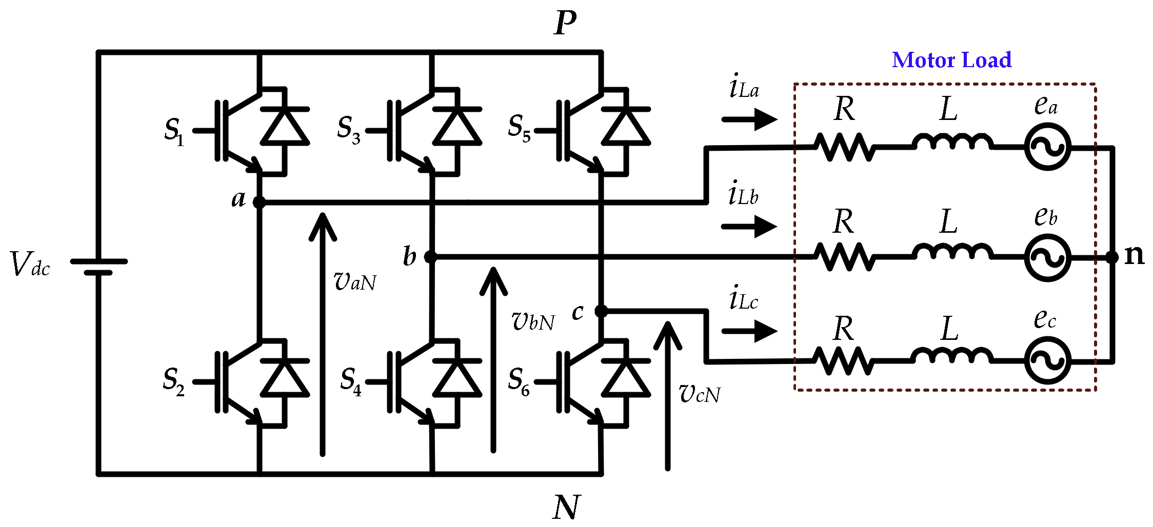
2.1. Inverter System

The power circuit of a three-phase VSI is shown in Figure 2, where V_dc is the dc voltage; v_aN, v_bN, and v_cN are the phase-to-neutral voltages of inverter; i_La, i_Lb, and i_Lc are the load currents; R is the load resistance; L is the load inductance; and e_a, e_b, and e_c are the back-EMF in each phase, respectively. The switching states are determined by the gating signals S_a, S_b, and S_c, as shown in

Table 1. Gating signals of inverter power switches.

Leg a, Sa	Leg b, Sb	Leg c, Sc
S1 ON, 1	S3 ON, 1	S5 ON, 1
S2 OFF, 0	S4 OFF, 0	S6 OFF, 0
S1 OFF, 0	S3 OFF, 0	S5 OFF, 0
S2 ON, 1	S4 ON, 1	S6 ON, 1

. The switching states S can be expressed in vector form as:

$$\mathit{S}=\frac{2}{3}\left(S_a+e^{j2\pi /3}{S}_b+e^{j4\pi /3}{S}_c\right)$$

(1)

The output voltage space vectors generated by the inverter are defined by:

$$v_i=\frac{2}{3}\left(v_{aN}+e^{j2\pi /3}{v}_{bN}+e^{j4\pi /3}{v}_{cN}\right)$$

(2)

Then, the load voltage vector v_i can be related to the switching state vector S by:

$${\mathit{v}}_{\mathit{i}}=\mathit{S}{V}_{dc}$$

(3)

Considering all possible switching combinations of gating signals, eight switching states and hence eight voltage vectors are obtained as shown in

Table 2. Voltage vectors for possible switching state.

vi	[Sa Sb Sc]	[vreal vimg]
v0	[0 0 0]	[0, 0]
v1	[1 0 0]	[2Vdc/3, 0]
v2	[0 1 0]	[−Vdc/3, √3 Vdc/3]
v3	[1 1 0]	[Vdc/3, √3Vdc/3]
v4	[0 0 1]	[−Vdc/3, −√3Vdc/3]
v5	[1 0 1]	[Vdc/3, −√3Vdc/3]
v6	[0 1 1]	[−2Vdc/3, 0]
v7	[1 1 1]	[0, 0]

. The load current dynamics can be expressed by the vector equation:

$${\mathit{v}}_{\mathit{i}}=R{i}_L+L\frac{d{i}_L}{dt}+e$$

(4)

where the balance three-phase load current i_L and the three-phase load back-EMF e can be represented in space vector form as:

$${\mathit{i}}_{\mathit{L}}=\frac{2}{3}\left(i_{La}+e^{j2\pi /3}{i}_{Lb}+e^{j4\pi /3}{i}_{Lc}\right)$$

(5)

$$\mathit{e}=\frac{2}{3}\left(e_a+e^{j2\pi /3}{e}_b+e^{j4\pi /3}{e}_c\right)$$

(6)

For simplicity and to reduce computational burden, the inverter voltage vector v_i, load current i_L, and back-EMF e can be represented in a stationary reference frame (α–β) as:

$${\mathit{v}}_{\mathit{i}}={\left[v_{i\alpha }{v}_{i\beta }\right]}^T{\mathit{i}}_{\mathit{L}}={\left[i_{L\alpha }{i}_{L\beta }\right]}^T\mathit{e}={\left[e_{\alpha }{e}_{\beta }\right]}^T$$

(7)

Using the Clark transformation, the relation between abc and αβ is given by:

$$\left[\begin{array}{c}{x}_{\alpha }\\ x_{\beta }\end{array}\right]=\frac{2}{3}\left[\begin{array}{ccc}1& -\frac{1}{2}& -\frac{1}{2}\\ 0& \frac{\sqrt{3}}{2}& -\frac{\sqrt{3}}{2}\end{array}\right]\left[\begin{array}{c}{x}_a\\ x_b\\ x_c\end{array}\right]$$

(8)

where x can be replaced by variables v_i, i_L, and e.

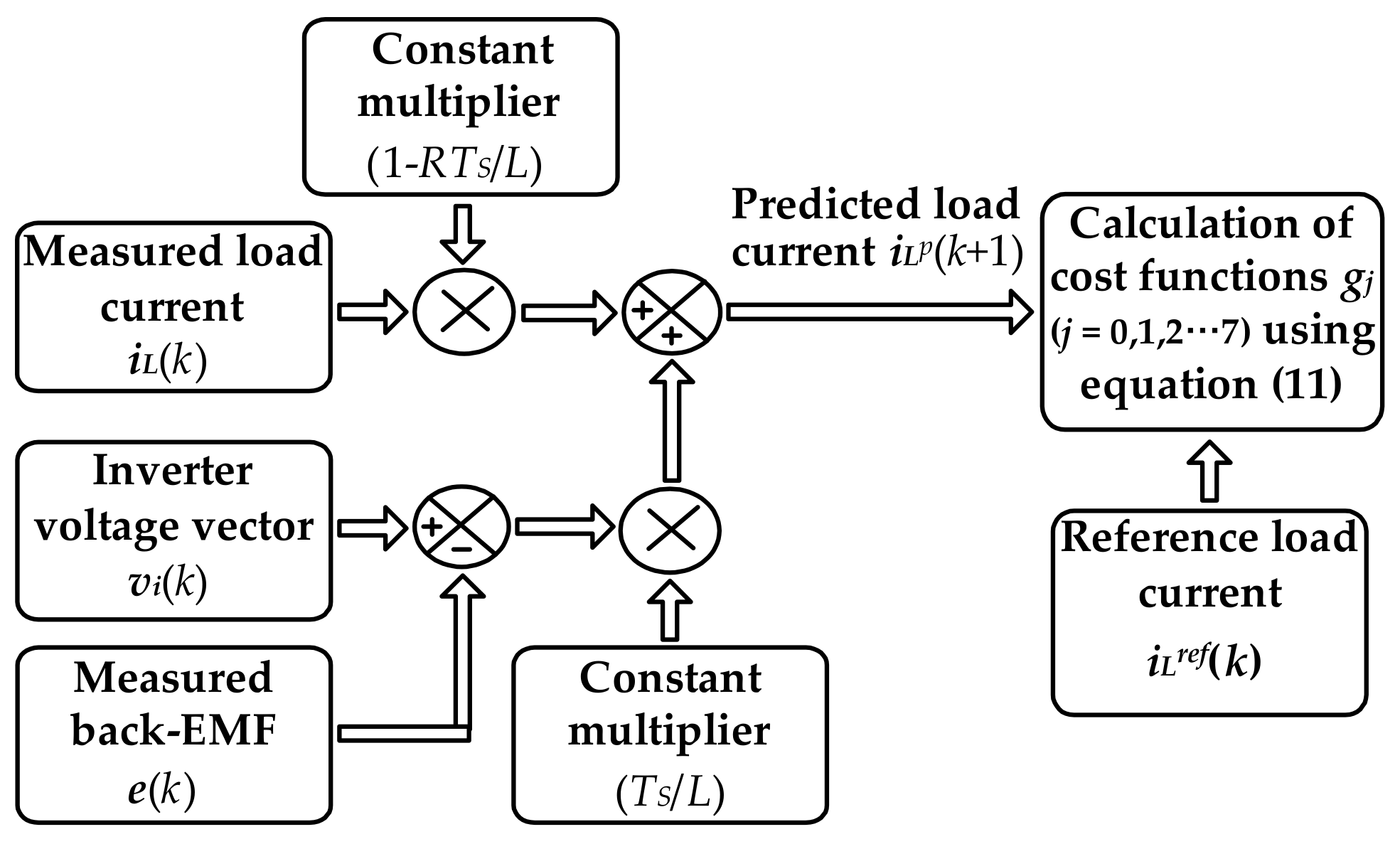
2.2. Predictive Model

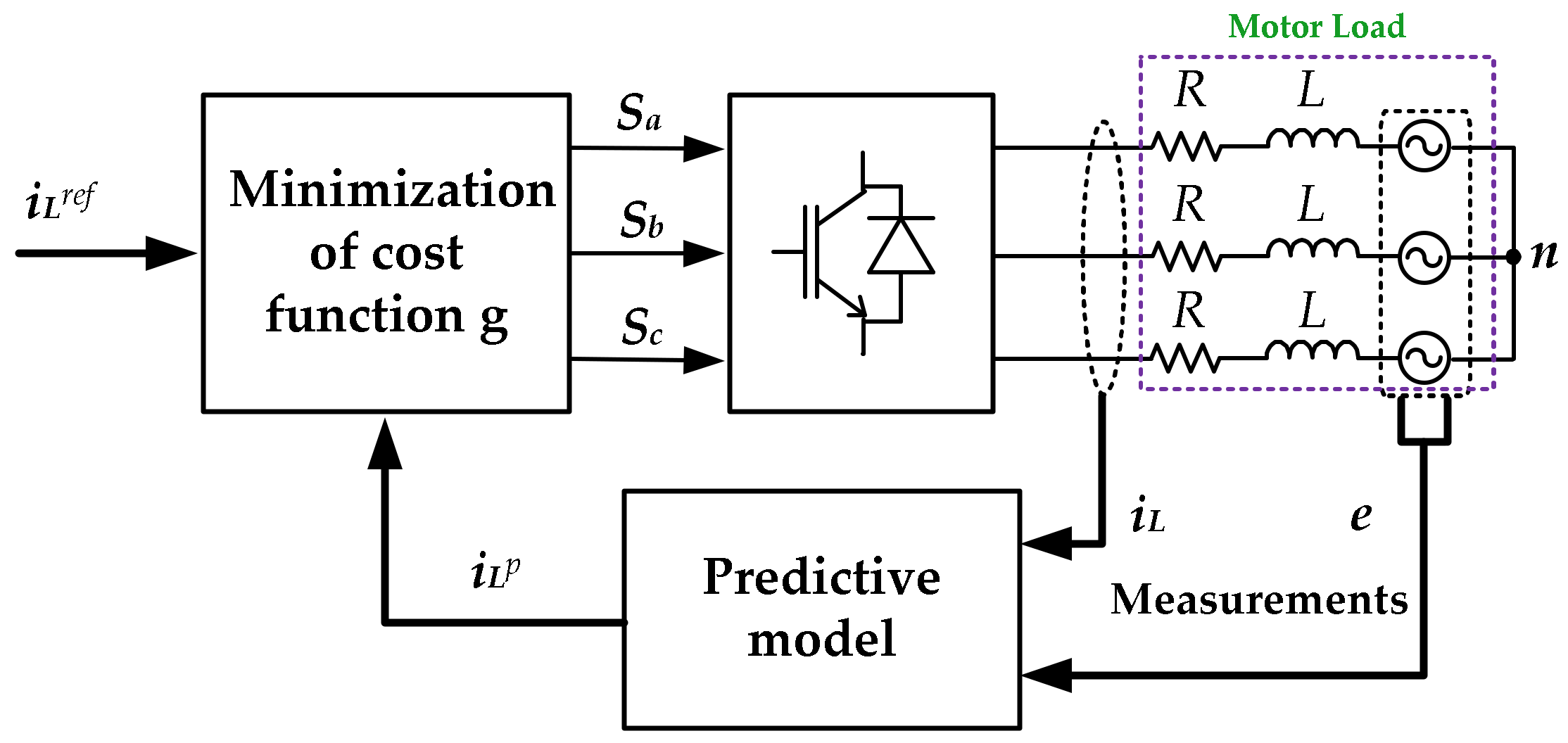
The discrete-time model of the load current dynamics continuous-time model (Equation (4)) for a sampling time T_S represents the predictive model. It is used for the future predictions of the load current from each voltage vectors and the measured load currents at the present sampling instant k. The discrete-time model can be obtained by a simple approximation of the load current derivative di_L/dt by using the forward Euler approximation, given as:

$$\frac{d{\mathit{i}}_{\mathit{L}}}{dt}\approx \frac{{\mathit{i}}_{\mathit{L}}(k+1)-{\mathit{i}}_{\mathit{L}}(k)}{T_S}$$

(9)

After substituting Equation (9) into Equation (4), an expression of the predicted future load current at the next sampling interval k + 1 can be obtained for each of the seven different voltage vectors v_i(k) generated by the inverter as:

$${{\mathit{i}}_L}^p\left(k+1\right)=\left(1-\frac{R{T}_S}{L}\right){\mathit{i}}_{\mathit{L}}\left(k\right)+\frac{T_S}{L}\left({\mathit{v}}_{\mathit{i}}\left(k\right)-\mathit{e}\left(k\right)\right)$$

(10)

where i_L^p(k + 1) denotes the predicted future load current at instant k + 1, i_L(k) is the measured load current at instant k, the inverter voltage v_i(k) is the decision variable to be calculated by the controller, and e(k) is the measured back-EMF voltage at the instant k. These predicted future load currents are used for the calculation of the cost function in the FS-MPC algorithm.

2.3. Cost Function

An objective function is required for the selection of the optimum switching state corresponding to a given sampling interval. The cost function is used in the case of MPC to compute the optimized switching state by minimizing the error between the reference and the measured current. The step-by-step explanation of the cost function is as follows:

• The value of reference current i_L^ref(k) is obtained from an outer control loop at the sampling instant k.
• The load current i_L(k) and the back-EMF voltage e(k) are measured at the sampling instant k.
• The discrete-time model of the load (Equation (10)) is used to predict the future value of the load current i_L^p(k + 1) in the next sampling instant k + 1 for each of the possible switching states of the inverter.
• Then, the cost function is evaluated for all the predicted load currents, which is a function of the reference current i^ref(k) and the predicted load current i_L^p(k + 1).
• The switching state which minimizes the cost function is selected and applied to the inverter in the next sampling interval.

The cost function can be expressed in the stationary reference frame (α–β) as:

$$g=\left|i_{L\alpha }^{ref}-i_{L\alpha }^p\left(k+1\right)\right|+\left|i_{L\beta }^{ref}-i_{L\beta }^p\left(k+1\right)\right|$$

(11)

where $i_{L\alpha }^{ref}$ and $i_{L\beta }^{ref}$ are the real and imaginary parts of reference current, and $i_{L\alpha }^p$ and $i_{L\beta }^p$ are the real and imaginary parts of the predicted load current vector i_L^p(k + 1), respectively.

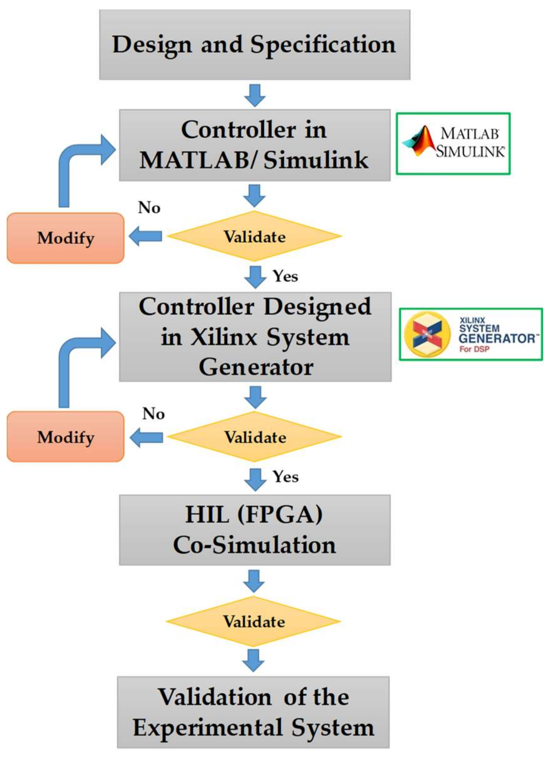
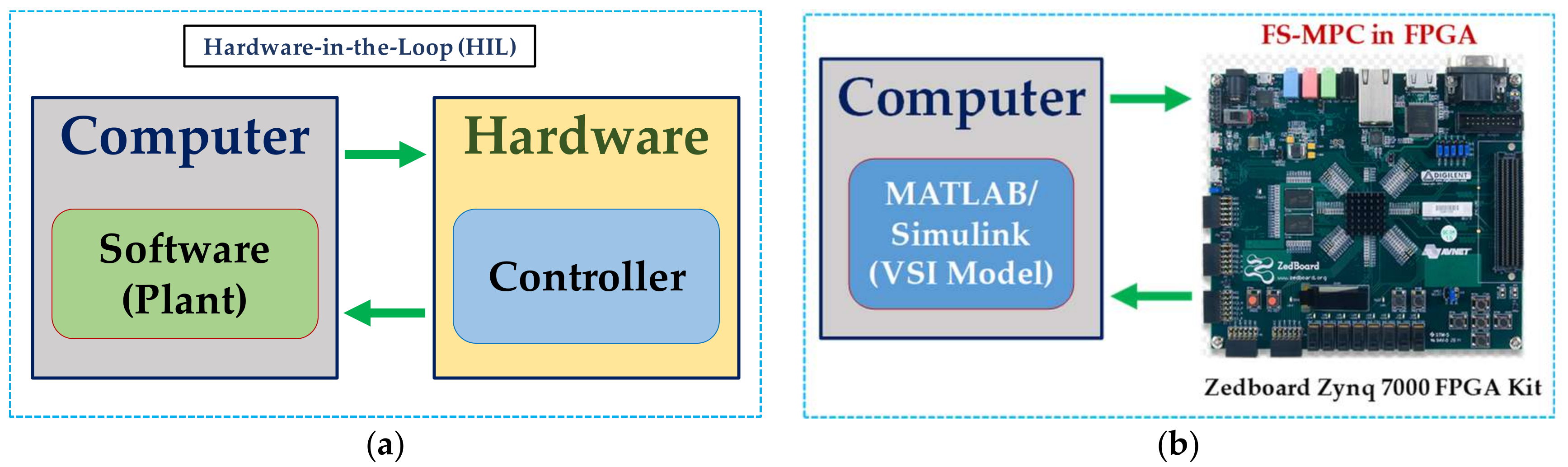
3. HIL Co-Simulation

HIL co-simulation provides an intermediate level of system verification between the software simulation and implementation of the controller on the actual experimental system. The flowchart of the HIL co-simulation using FPGA is shown in Figure 3. At the initial stage, the controller and VSI system are modelled in MATLAB/Simulink and the performance is verified using simulations. Furthermore, the controller modelling is developed using the XSG digital platform and the performance is analyzed considering the model of the control using Simulink. The digital modelling of the controller is validated at the later stage through the real-time HIL co-simulation.

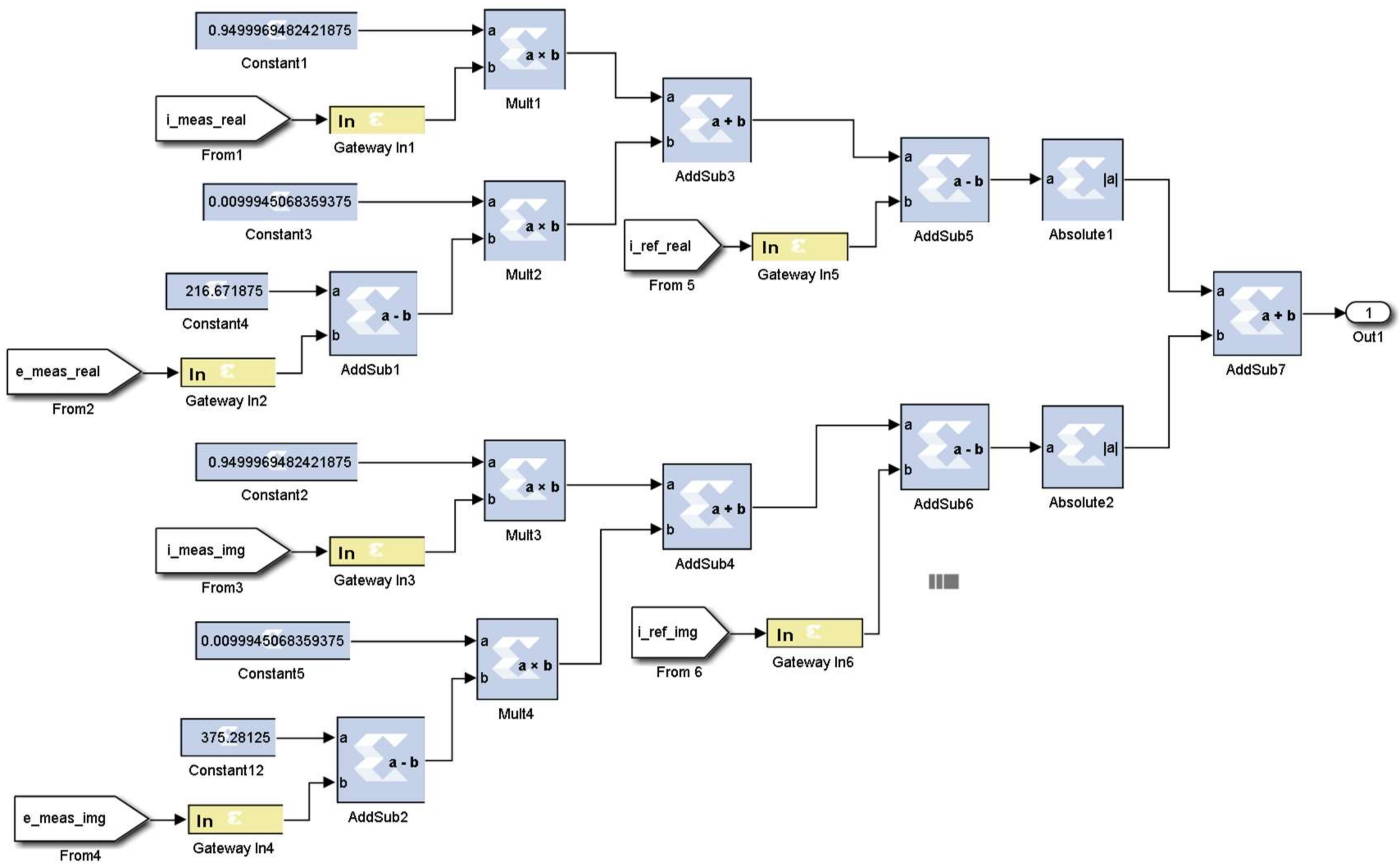
3.1. Modelling of the FS-MPC in XSG

The implemented controller in the MATLAB/Simulink platform is required to be modelled for the digital implementation of the controller in the XSG environment. The implementation of the FS-MPC in XSG is performed using the Xilinx blockset available in MATLAB/Simulink. The XSG provides a virtual FPGA platform to perform the HIL co-simulation. The modelling of the controller is described in following two sections.

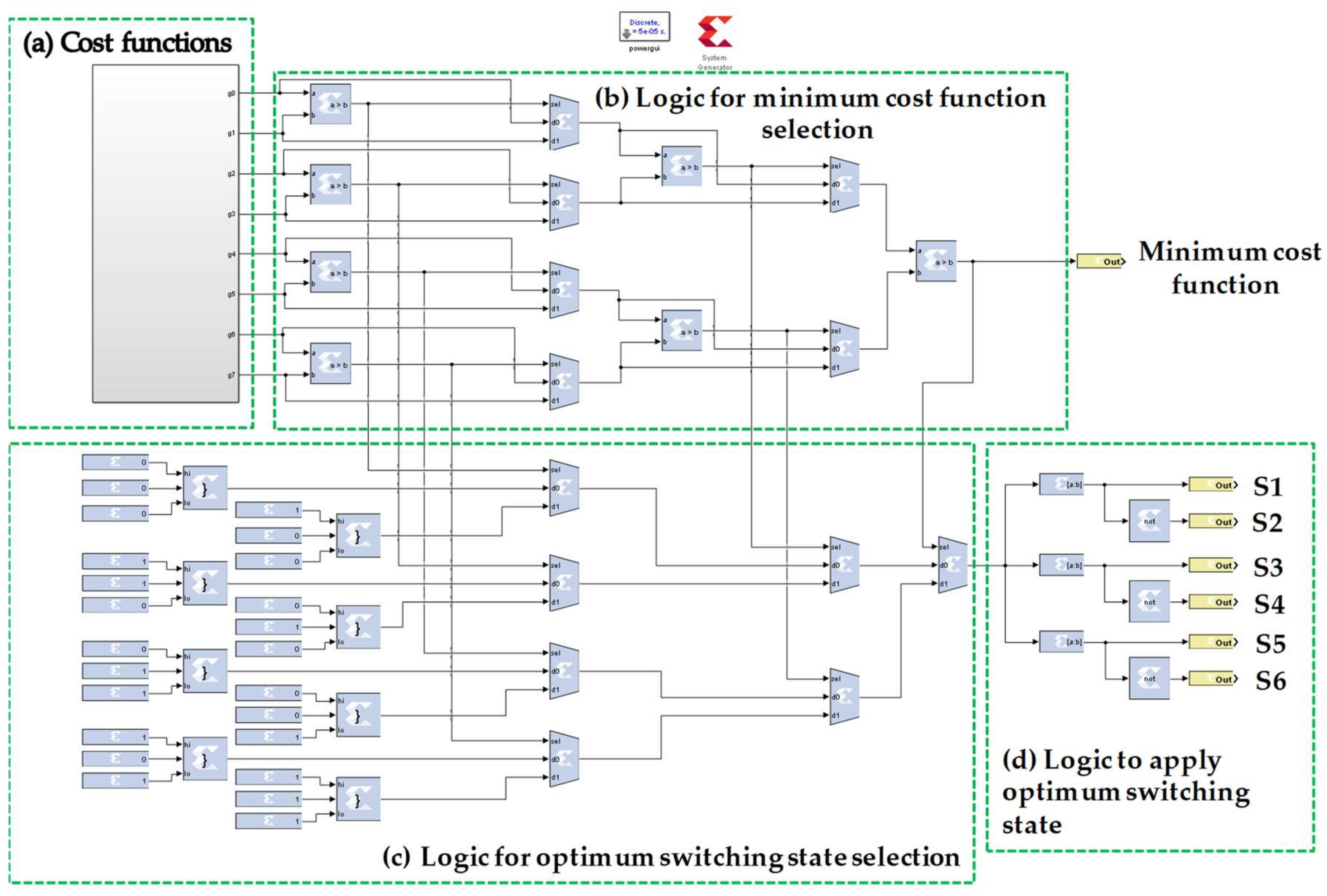
3.1.1. Computation of the Cost Function

The block diagram for the calculation of cost functions is shown in Figure 4. Initially, the predicted load current is modelled using Equation (10) considering a voltage vector for the three-phase VSI. Finally, the cost function is computed using Equation (11) for the respective predicted load currents. The modelling for the computation of the cost function in Figure 5 is developed in the XSG platform. The measured variables i_L(k) and e(k) are used as inputs to compute predicted load currents i_L^p(k + 1) corresponding to each voltage vectors v_i(k). Furthermore, the cost functions corresponding to different voltage vectors are calculated by feeding the predicted load currents and reference current i_L^ref(k). The cost function corresponding to each output voltage vector (v₀–v₇) is computed simultaneously through the modelling.

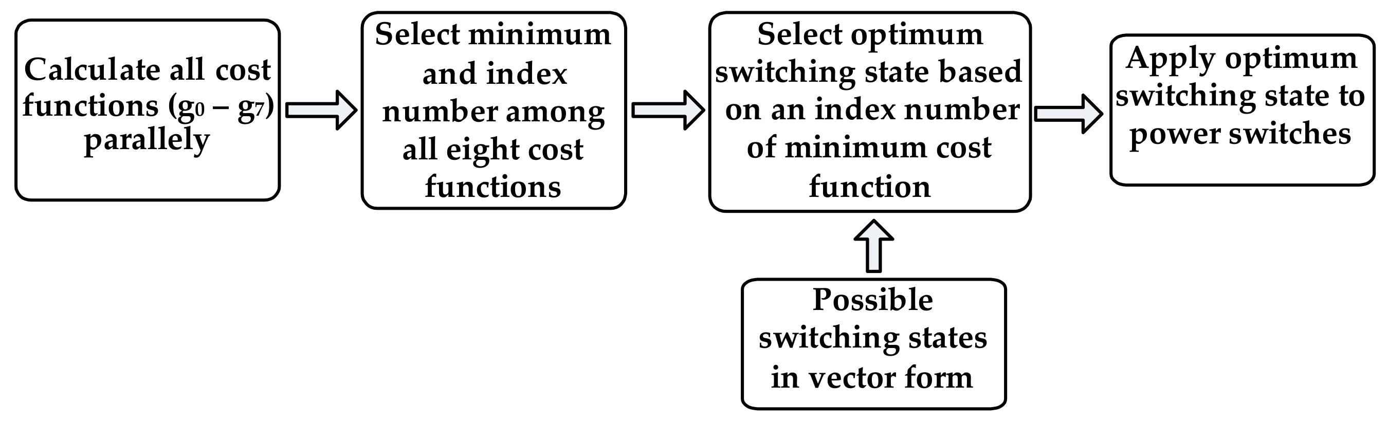
3.1.2. Selection of Optimum Switching Signals

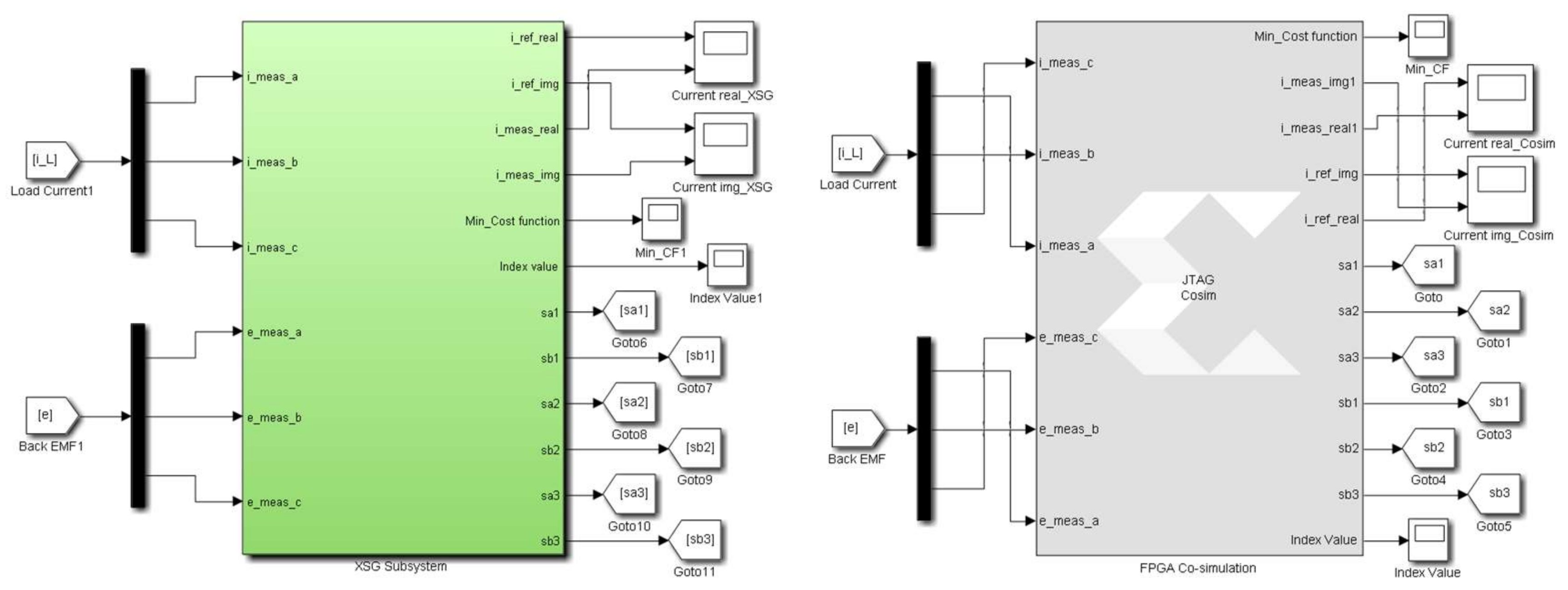
The modelling for the selection of the optimum switching state is developed based upon the block diagram in Figure 6. The index number 0–7 is defined for each of the voltage vectors v₀–v₇, respectively. The computed cost functions are further utilized for the selection of the index number corresponding to the minimized cost function. The switching state for the minimized cost function is selected as per the index number according to a 3 × 8 matrix of possible switching states. The modelling for selection of the minimum cost function for the optimum switching state is implemented as in Figure 7, and the generated switching signals are applied to the VSI.

3.2. Co-simulation

In this paper, HIL co-simulation is considered for the validation of the controller by implementing it on the hardware system through the interaction with the software system as shown in Figure 8a. The co-simulation is performed using FPGA as an actual hardware by interacting with a computer as shown in Figure 8b. Firstly, the modelling of the controller is developed in the XSG, and further validation is performed using the co-simulation functionality of the XSG platform. The HIL co-simulation is performed by implementing the FS-MPC in the FPGA through its interaction with the VSI system in MATLAB/Simulink as represented in Figure 8b. The co-simulation prototype block is generated by selecting the appropriate FPGA evaluation board using the XSG token in MATLAB/Simulink. The co-simulation prototype block enables the MATLAB/Simulink system to interact with the FPGA. The signal ports are assigned in the co-simulation block corresponding to the input signal from Simulink to the XSG and output signal from the XSG to Simulink.

The co-simulation block of the FS-MPC contains the FPGA files that are programmed in the FPGA while performing a co-simulation, and the input–output signals are exchanged between the FPGA and MATLAB/Simulink. The co-simulation block is generated through the digital system modelling in the XSG as shown in Figure 9. Signal ports of the VSI system are connected through the signal ports assigned for the co-simulation block in MATLAB/Simulink. The validation of the controller system through co-simulation is performed using the Zedboard Zynq evaluation and development FPGA kit. The FPGA kit is physically connected to computer using a micro-USB cable that connects the joint test action group (JTAG) port available in the FPGA and a USB port available in the computer to perform HIL co-simulation.

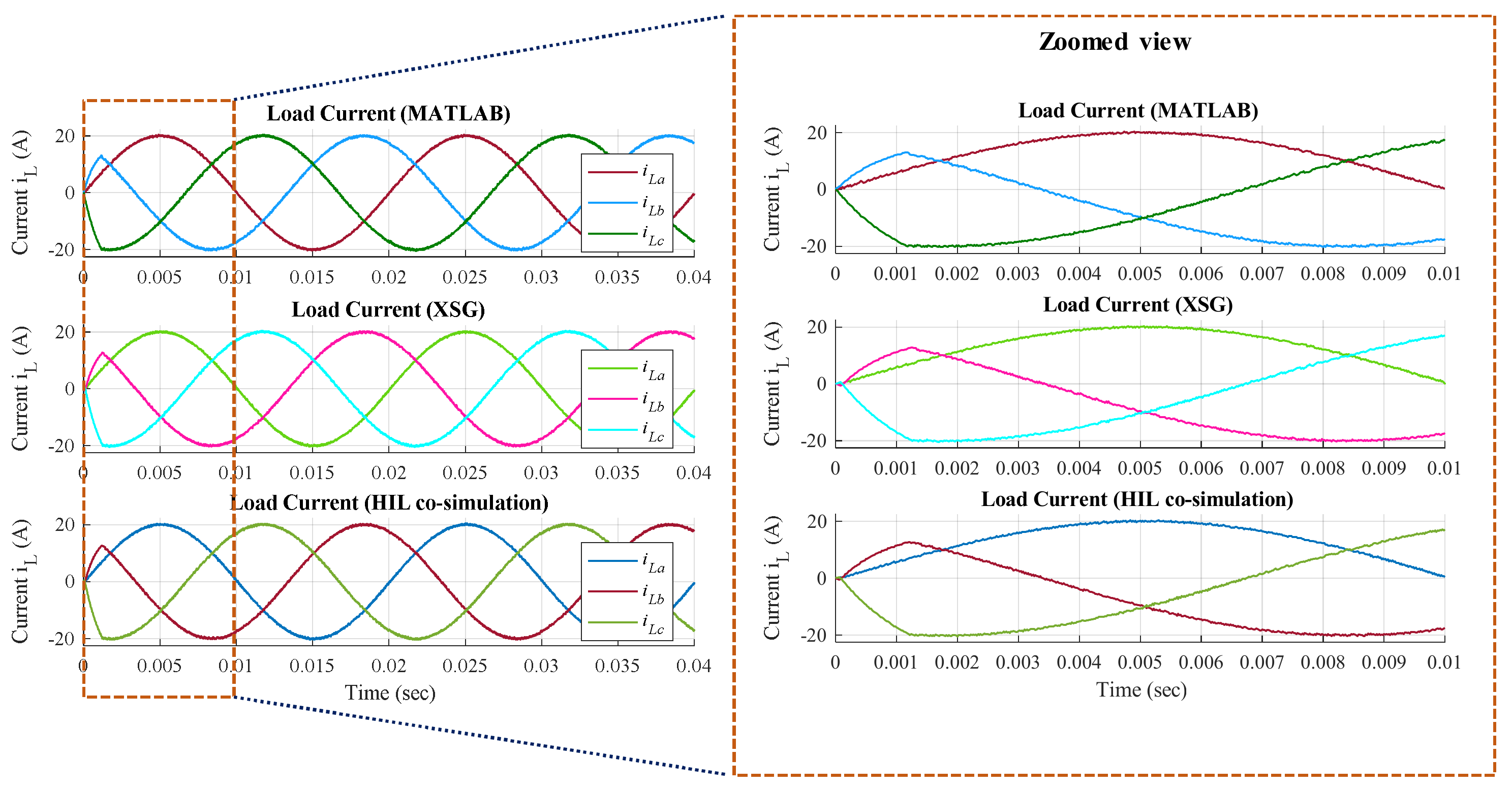
4. Results and Discussion

The performance of the three-phase VSI system is validated through the implementation of a controller in MATLAB/Simulink as well as XSG environments and HIL co-simulation. The parameters considered for the VSI system with a motor-type load are depicted in

Table 3. Parameters for VSI system.

Description	Parameter	Value
DC supply voltage	Vdc	650 V
Load resistor	R	10 Ω
Load inductor	L	10 mH
Sinusoidal back-EMF	e	100 V
Frequency	f	50 Hz
Sampling period	TS	50 µs

. The system performance is analyzed considering intermediate results: minimum cost function-index value, sampling time, and tracking performance.

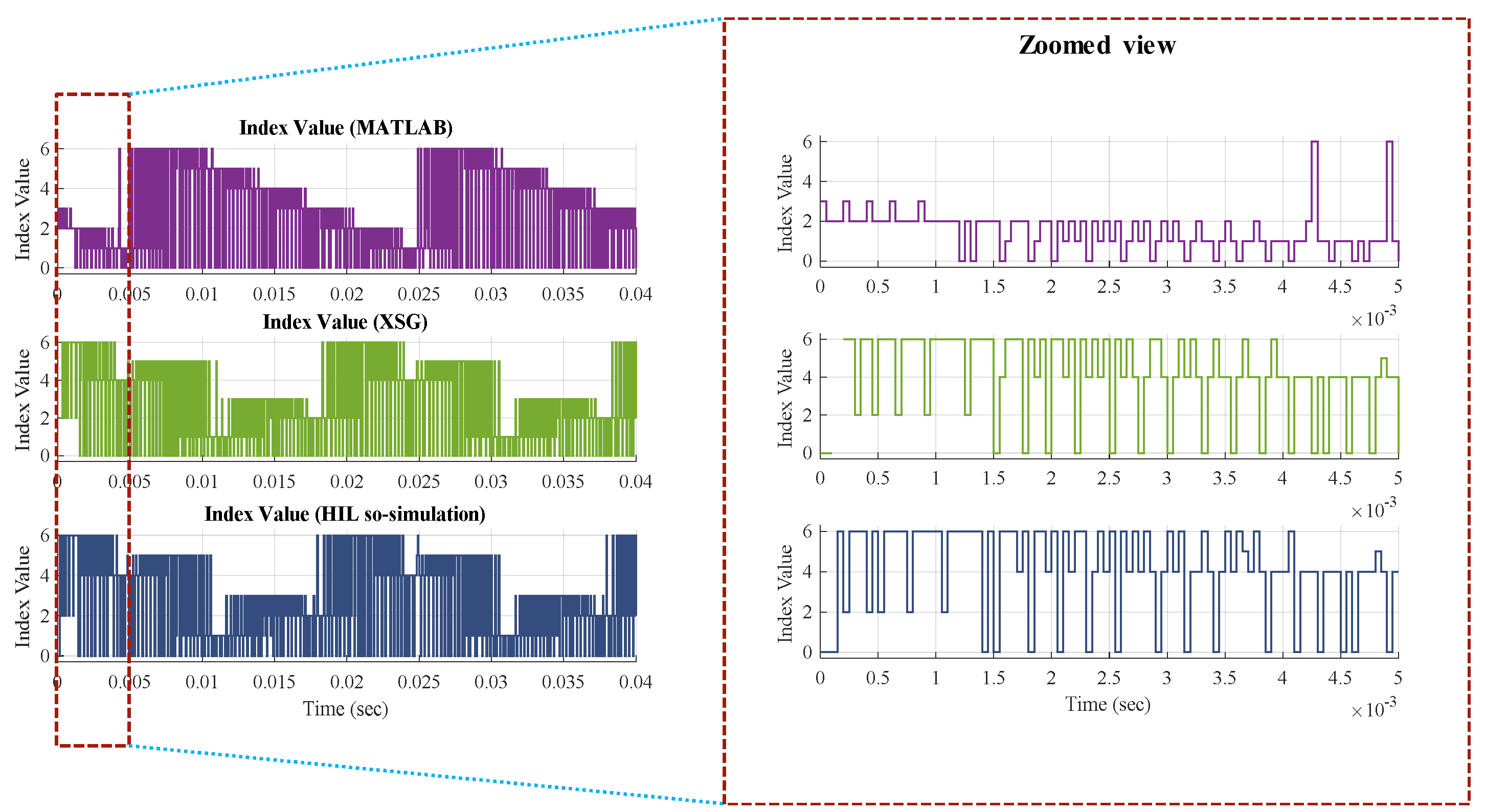
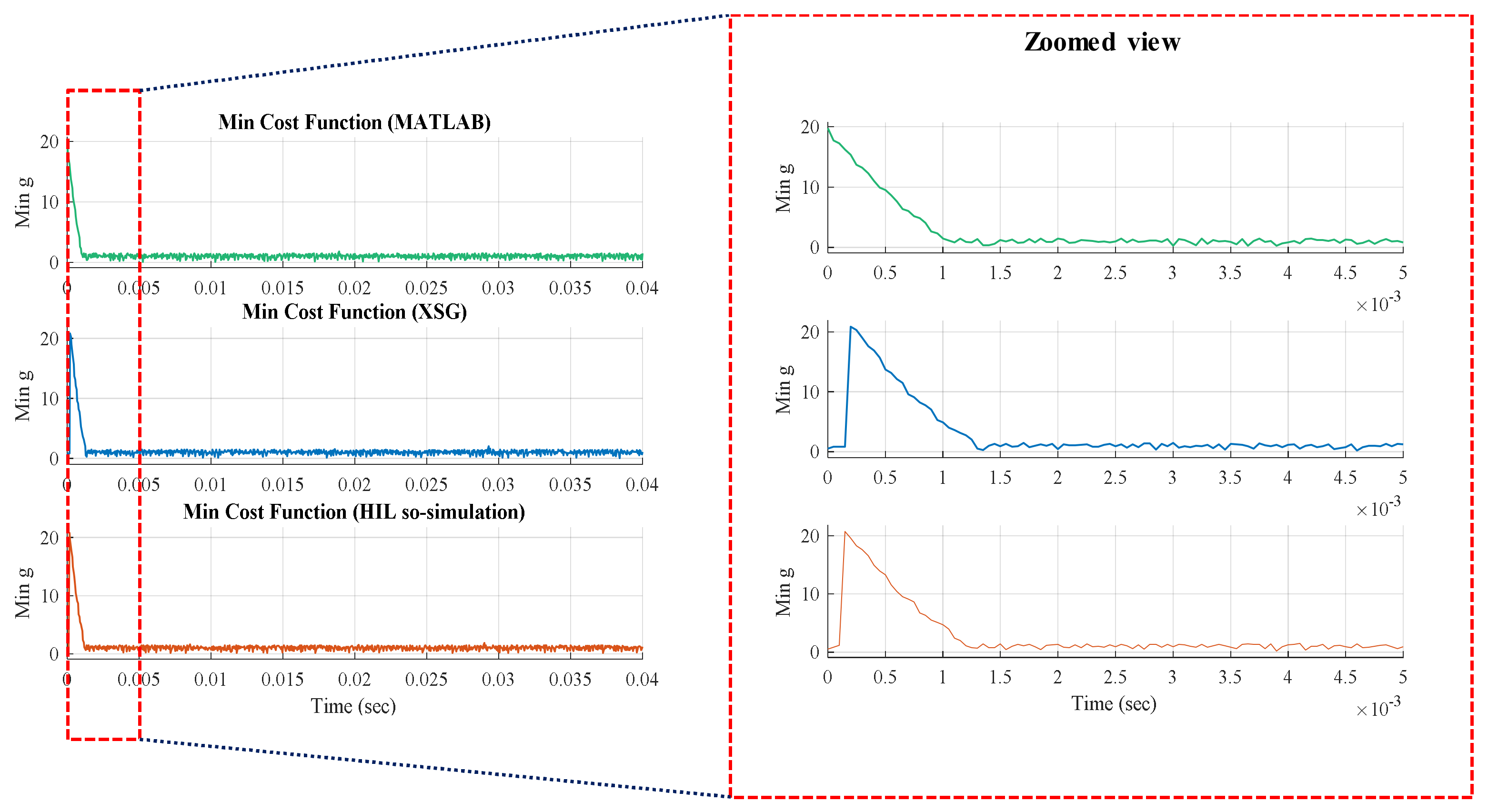
4.1. Intermediate Response

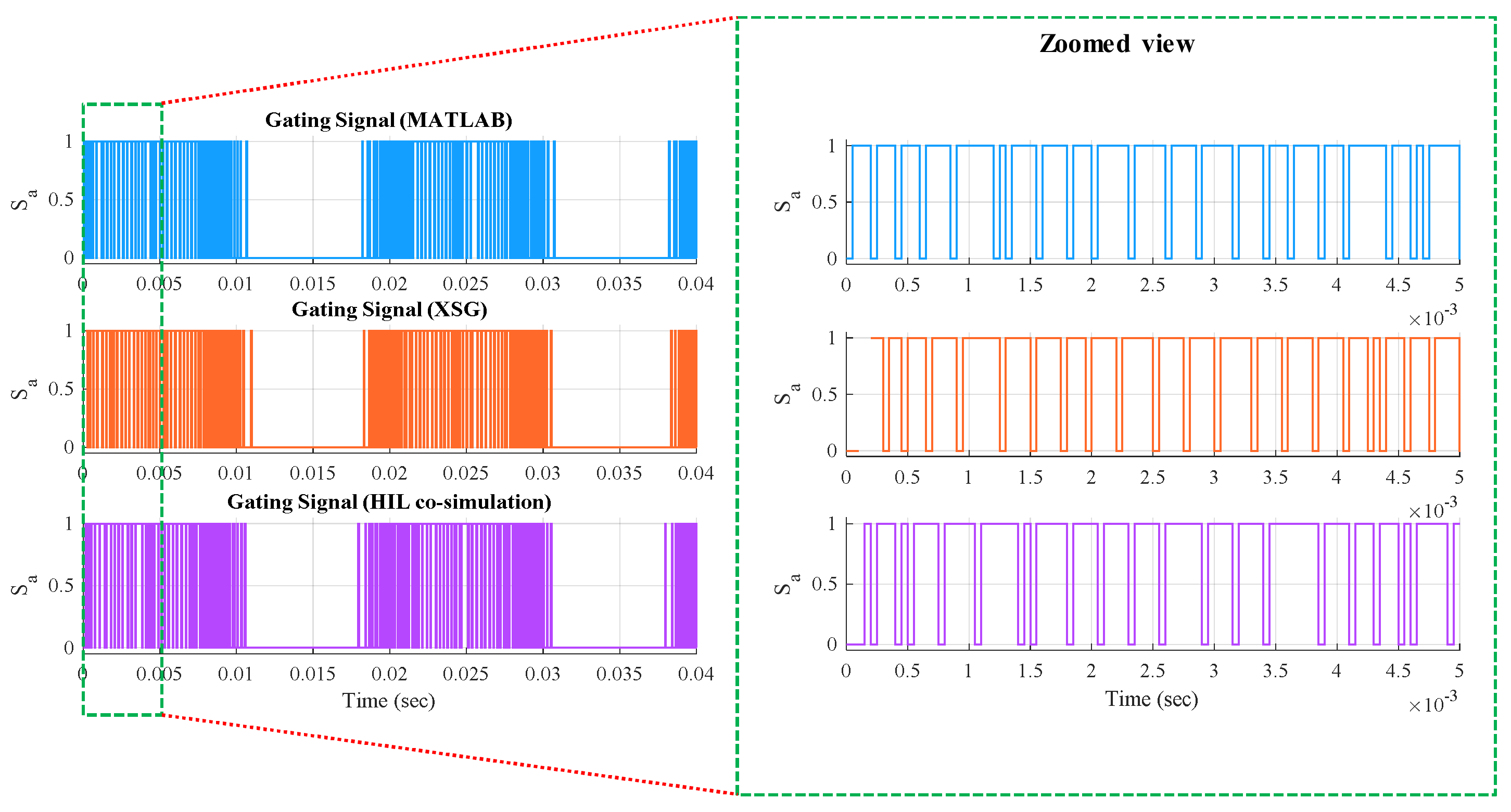
The intermediate responses of the selection of the minimum cost function and the index number corresponding to the optimum switching state are analyzed for the modelling and implementation of the FS-MPC. A sampling time of 50 µs was chosen for the selection of the minimum cost function for each sampling interval as depicted in Figure 10. The minimum cost function response results in the minimized current error. The minimized current error is required for improved performance of the system to feed quality power output. The selection of the index number for an optimum switching state in Figure 11 is represented for each sampling interval.

The intermediate responses for Simulink is different as compared to the XSG and HIL co-simulation platforms. The responses for the XSG and HIL co-simulation is quite similar due to digital-based platform. The small difference observed in the XSG and HIL co-simulation might be due to the prompt response during co-simulation as the controller is operating in real-time through the FPGA. The prompt response of the controller for co-simulation as compared to the XSG can be observed for the selection of the minimum cost function in Figure 10. Furthermore, the switching signals are generated corresponding to the index number selection in each sampling interval that will be applied to the VSI. The switching signals in Figure 12 are demonstrated for the leg “a” upper switch of the VSI, considering the controller implementation in all three platforms.

4.2. Sampling Time

The performance of the controller depends on the sampling time T_S selected for the discretization of the continuous-time model. Different sampling time T_S is considered for the discretization of the VSI system to analyze and validate the performance of the controller. The sampling time T_S governs the maximum switching frequency that is half of the sampling frequency. Therefore, the increase in T_S results in the decrease in the maximum switching frequency of the VSI system, and vice versa. The operation of the FS-MPC is considered for T_S = 20, 50, and 100 µs to analyze the effect of T_S. In addition, the effect of change in T_S is compared for the implementation of the FS-MPC in MATLAB/Simulink, XSG, and HIL co-simulation. The load currents are demonstrated for T_S = 50 µs in Figure 13, T_S = 100 µs in Figure 14, and T_S = 20 µs in Figure 15.

The load current for the steady state condition is almost similar for the implementation using all three platforms. However, the transient performances are not similar for the MATLAB/Simulink and HIL co-simulation, as demonstrated in the enlarged view of the load currents. The controller performance is delayed in case of HIL co-simulation for all the sampling times considered for the demonstration. Furthermore, the similar controller response for XSG and HIL co-simulation during transient conditions verified that the delay is due to the response of the controller rather than delay introduced due to the interaction of the actual hardware and computer. The delay in response is higher for a high sampling time due to the operation of the controller at a low sampling frequency.

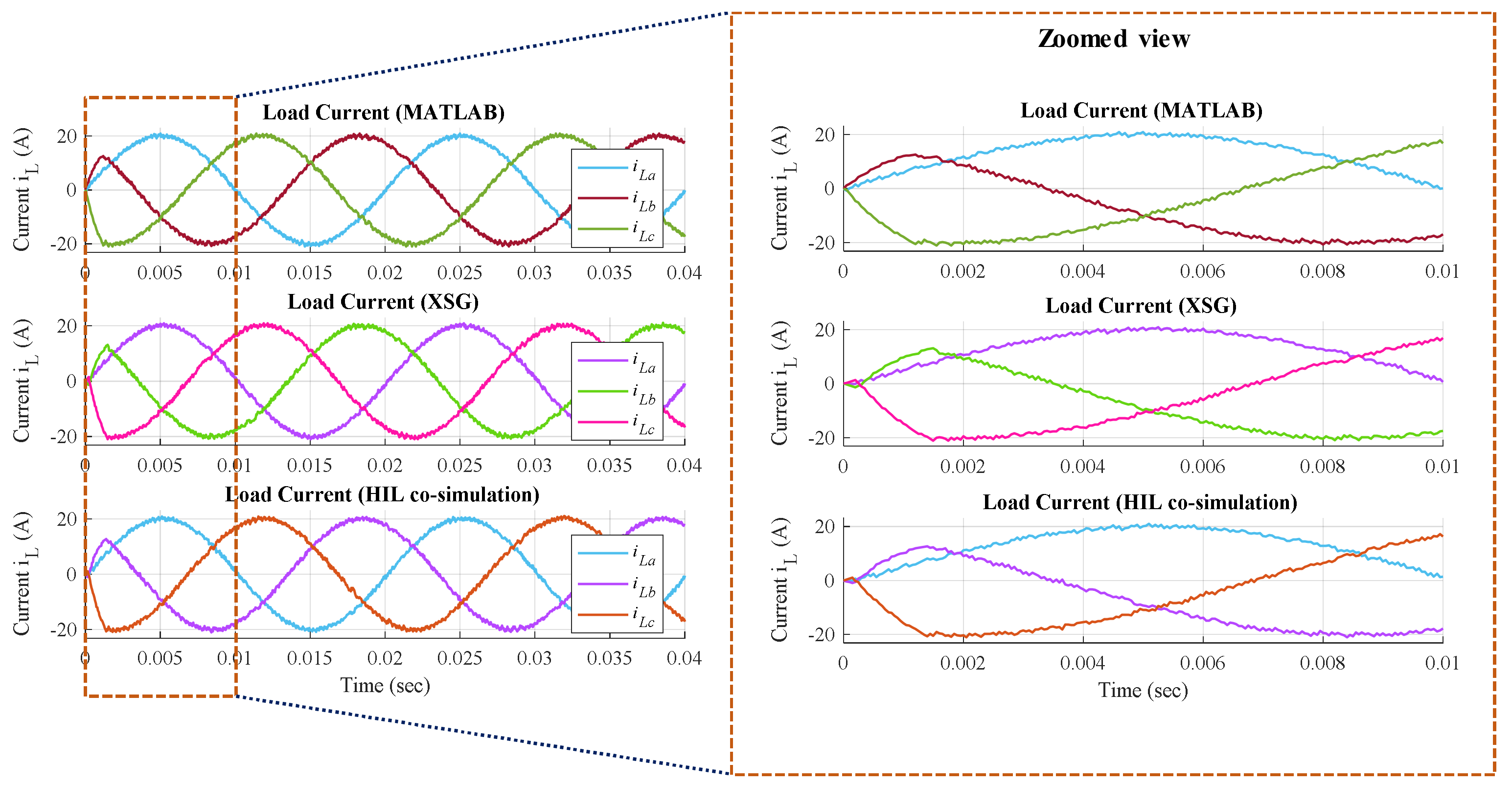
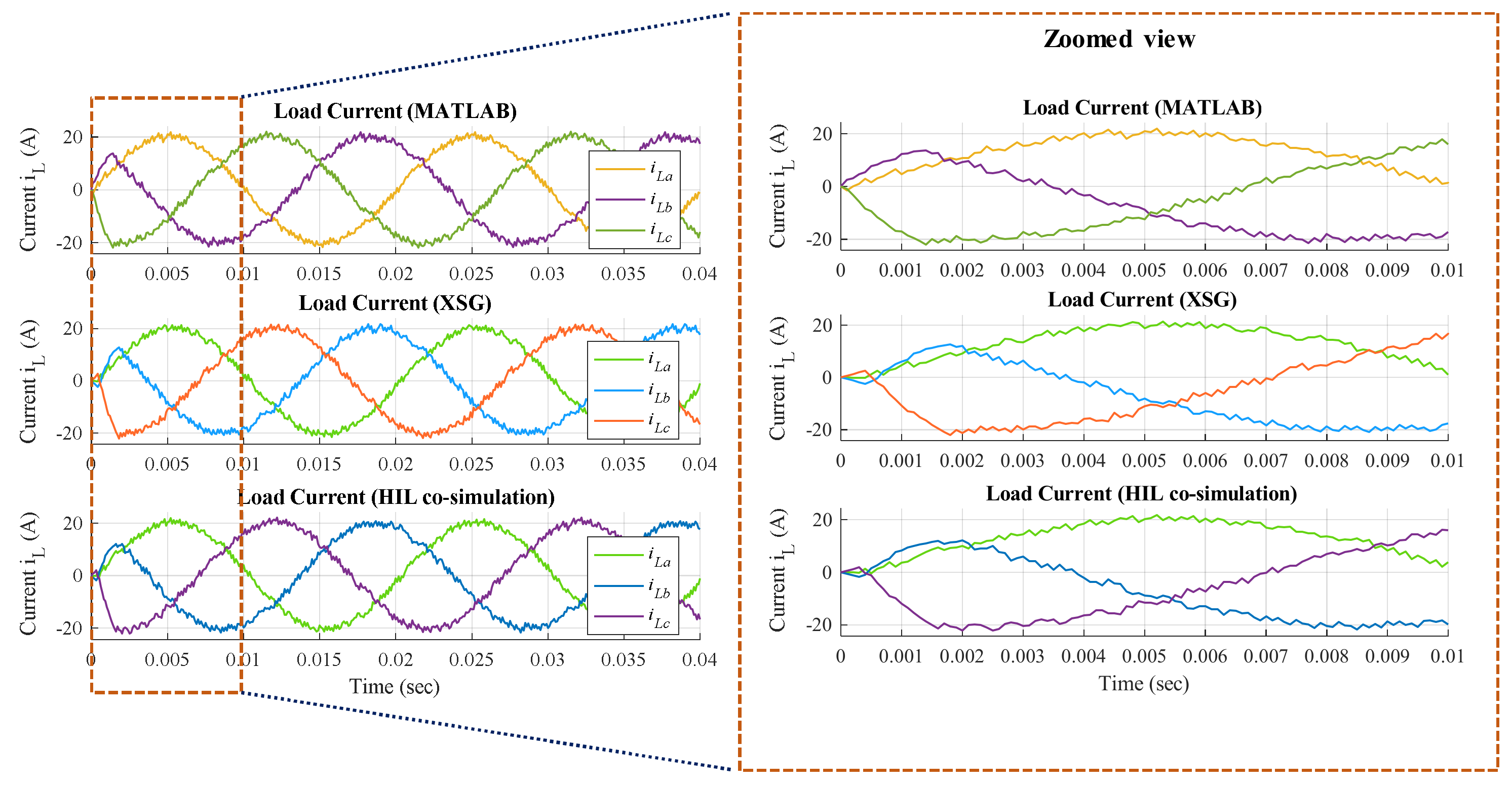
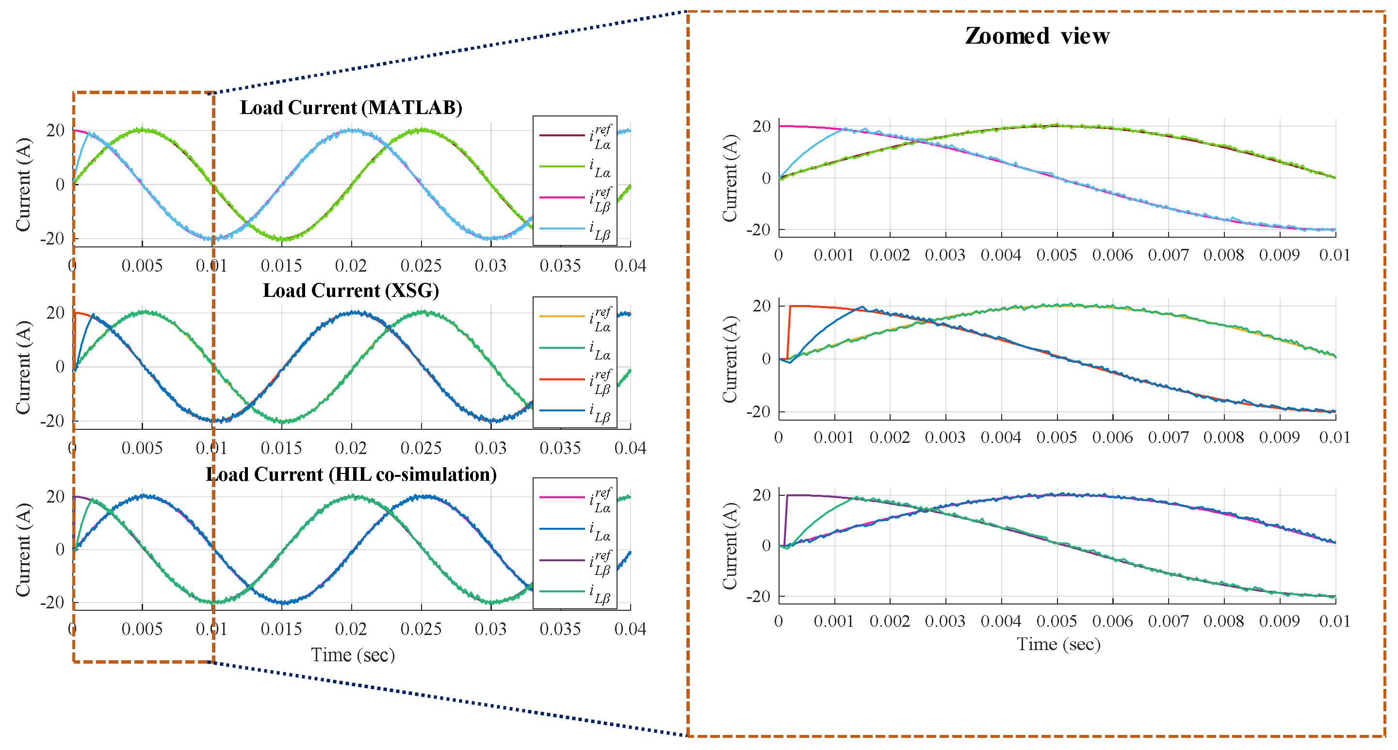
4.3. Tracking Performance

The tracking of the load current with respect to the reference is a significant characteristic to analyze the performance of a given controller. The tracking of the load current real component (i_Lα) and imaginary component (i_Lβ) with respect to the sinusoidal reference current is demonstrated in Figure 16 for the sampling time T_S = 50 µs. The tracking performance is analyzed during transient conditions due to perturbation in the reference current, as in Figure 17, to demonstrate the dynamic response of the controller. The good tracking performance is obtained as the load current properly tracks the reference current at each moment during the normal operating conditions as well as during the transient condition. An extreme transient case is considered: change in magnitude and phase at the same instant with respect to normal operating conditions.

The tracking performance for all three platforms are similar under normal operating conditions as well as under dynamic conditions. However, the slight delay in response for the XSG and HIL co-simulation compared to the MATLAB/Simulink platform can be seen in the enlarged view as shown in Figure 16. However, there is no delay in response for XSG and HIL co-simulation, which indicates the advantage of co-simulation through the operation of the controller in a real-time environment.

5. Conclusions

This paper presents the FS-MPC modelled in XSG and tested through HIL co-simulation using an FPGA for controlled power conversion through a three-phase VSI system considered with a motor load condition. The design and development of efficient controllers are required for controlled power conversion through VSI to use power generated from renewable energy sources. The FS-MPC has gained attention in the field of power electronic and drives for controlled power conversion, possessing the discrete nature of control that readily suits implementation in a digital environment. The FS-MPC is implemented in MATLAB/Simulink and further in an XSG platform that is used for digital system design. The controller performance is validated for a real-time environment through a HIL co-simulation considering the step-by-step analysis through intermediate outputs: the minimum cost function and selection of an index number. Also, the performance is validated considering the effect of the sampling time and tracking performance under dynamic conditions. The modelling of the FS-MPC in XSG is a viable choice due to the discrete nature of the controller. Furthermore, the real-time HIL co-simulation is a realistic approach for implementation by validating the controller performance before applying it to a real experimental system, to reduce the risk of component damage/whole system failure. In the future, the integrated platform of MATLAB/Simulink-XSG will be used to generate HDL codes for the implementation of FS-MPC in real-time experimental systems using an FPGA. The FS-MPC-controlled VSI system will further be employed for the islanded and grid-connected application of solar photovoltaic systems.

References

1. Bak, Y.; Lee, J.-S.; Lee, K.-B. Low-voltage ride-through control strategy for a grid-connected energy storage system. Appl. Sci. 2018, 8, 57. [Google Scholar] [CrossRef]
2. Tahir, S.; Wang, J.; Baloch, M.H.; Kaloi, G.S. Digital control techniques based on voltage source inverters in renewable energy applications: A Review. Electronics 2018, 7, 18. [Google Scholar] [CrossRef]
3. Smadi, I.A.; Albatran, S.; Ahmad, H.J. On the performance optimization of two-level three-phase grid-feeding voltage-source inverters. Energies 2018, 11, 400. [Google Scholar] [CrossRef]
4. Kazmierkowski, M.P.; Krishnan, R.; Blaabjerg, F. Control in Power Electronics, 1st ed.; Academic Press: New York, NY, USA, 2002. [Google Scholar]
5. Mohan, M.N.; Undeland, T.M.; Robbins, W.P. Power Electronics: Converters, Applications, and Design, 2nd ed.; Wiley: New York, NY, USA, 1995. [Google Scholar]
6. Kazmierkowski, M.P.; Malesani, L. Current control techniques for three-phase voltage-source PWM converters: A survey. IEEE Trans. Ind. Electron. 1998, 45, 691–703. [Google Scholar] [CrossRef]
7. Brod, D.M.; Novotny, D.M. Current control of VSI-PWM inverters. IEEE Trans. Ind. Appl. IA-21, 562–570. [CrossRef]
8. Holtz, J. Pulse width modulation-a survey. IEEE Trans. Ind. Electron. 1992, 39, 410–420. [Google Scholar] [CrossRef]
9. Ho, C.N.M.; Cheung, V.S.P.; Chung, H.S.H. Constant-frequency hysteresis current control of grid-connected VSI without bandwidth control. IEEE Trans. Power Electron. 2009, 24, 2484–2495. [Google Scholar] [CrossRef]
10. Geyer, T. A comparison of control and modulation schemes for medium-voltage drives: Emerging predictive control concepts versus PWM-based schemes. IEEE Trans. Ind. Appl. 2011, 47, 1380–1389. [Google Scholar] [CrossRef]
11. Cortes, P.; Kazmierkowski, M.P.; Kennel, R.M.; Quevedo, D.E.; Rodriguez, J. Predictive control in power electronics and drives. IEEE Trans. Ind. Electron. 2008, 55, 4312–4324. [Google Scholar] [CrossRef]
12. Kouro, S.; Cortes, P.; Vargas, R.; Ammann, U.; Rodriguez, J. Model predictive control—A simple and powerful method to control power converters. IEEE Trans. Ind. Electron. 2009, 56, 1826–1838. [Google Scholar] [CrossRef]
13. Rodríguez, J.; Cortes, P. Predictive Control of Power Converters and Electrical Drives, 1st ed.; Wiley-IEEE Press: New York, NY, USA, 2012. [Google Scholar]
14. Vazquez, S.; Rodriguez, J.; Rivera, M.; Franquelo, L.G.; Norambuena, M. Model predictive control for power converters and drives: Advances and trends. IEEE Trans. Ind. Electron. 2017, 64, 935–947. [Google Scholar] [CrossRef]
15. Rodríguez, J.; Pontt, J.; Cortés, P.; Vargas, R. Predictive control of a three-phase neutral point clamped inverter. In Proceedings of the Power Electronics Specialists Conference, Recife, Brazil, 12–16 June 2005. [Google Scholar]
16. Rodríguez, J.; Kazmierkowski, M.P.; Espinoza, J.R.; Zanchetta, P.; Abu-Rub, H.; Young, H.A.; Rojas, C.A. State of the art of finite control set model predictive control in power electronics. IEEE Trans. Ind. Inf. 2013, 9, 1003–1016. [Google Scholar] [CrossRef]
17. Cortes, P.; Rodriguez, J.; Antoniewicz, P.; Kazmierkowski, M. Direct power control of an AFE using predictive control. IEEE Trans. Power Electron. 2008, 23, 2516–2523. [Google Scholar] [CrossRef]
18. Perez, M.A.; Cortes, P.; Rodriguez, J. Predictive control algorithm technique for multilevel asymmetric cascaded H-bridge inverters. IEEE Trans. Ind. Electron. 2008, 55, 4354–4361. [Google Scholar] [CrossRef]
19. Cortes, P.; Wilson, A.; Kouro, S.; Rodriguez, J.; Abu-Rub, H. Model predictive control of multilevel cascaded H-bridge inverters. IEEE Trans. Ind. Electron. 2010, 57, 2691–2699. [Google Scholar] [CrossRef]
20. Lezana, P.; Aguilera, R.P.; Quevedo, D.E. Model predictive control of an asymmetric flying capacitor converter. IEEE Trans. Ind. Electron. 2009, 56, 1839–1846. [Google Scholar] [CrossRef]
21. Rivera, M.; Rojas, C.A.; Rodriguez, J.; Wheeler, P.; Wu, B.; Espinoza, J.R. Predictive current control with input filter resonance mitigation for a direct matrix converter. IEEE Trans. Power Electron. 2011, 26, 2794–2803. [Google Scholar] [CrossRef]
22. Rodríguez, J.; Pontt, J.; Silva, C.; Correa, P.; Lezana, P.; Cortés, P.; Ammann, U. Predictive current control of a voltage source inverter. IEEE Trans. Ind. Electron. 2007, 54, 495–503. [Google Scholar] [CrossRef]
23. Kouro, S.; Perez, M.A.; Rodriguez, J.; Llor, A.M.; Young, H.A. Model predictive control: MPC’s role in the evolution of power electronics. IEEE Ind. Electron. Mag. 2014, 8, 16–31. [Google Scholar] [CrossRef]
24. Vazquez, S.; Leon, J.I.; Franquelo, L.G.; Rodriguez, J.; Young, H.A.; Marquez, A.; Zanchetta, P. Model predictive control: A review of its applications in power electronics. IEEE Ind. Electron. Mag. 2015, 9, 8–21. [Google Scholar] [CrossRef] [Green Version]
25. Xia, C.; Liu, T.; Shi, T.; Song, Z. A simplified finite-control-set model-predictive control for power converters. IEEE Trans. Ind. Inf. 2014, 10, 991–1002. [Google Scholar]
26. Cortes, P.; Ortiz, G.; Yuz, J.; Rodríguez, J.; Vazquez, S.; Franquelo, L. Model predictive control of an inverter with output LC filter for UPS applications. IEEE Trans. Ind. Electron. 2009, 56, 1875–1883. [Google Scholar] [CrossRef]
27. Naouar, M.W.; Naassani, A.A.; Monmasson, E.; Slama-Belkhodja, I. FPGA-based predictive current controller for synchronous machine speed drive. IEEE Trans. Power Electron. 2008, 23, 2115–2126. [Google Scholar] [CrossRef]
28. Sanchez, P.M.; Machado, O.; Peña, E.J.B.; Rodríguez, F.J.; Meca, F.J. FPGA-based implementation of a predictive current controller for power converters. IEEE Trans. Ind. Inf. 2013, 9, 1312–1321. [Google Scholar] [CrossRef]
29. Selvamuthukumaran, R.; Gupta, R. Rapid prototyping of power electronics converters for photovoltaic system application using Xilinx System Generator. IET Power Electron. 2014, 7, 2269–2278. [Google Scholar] [CrossRef]
30. Monti, A.; Santi, E.; Dougal, R.A.; Riva, M. Rapid prototyping of digital controls for power electronics. IEEE Trans. Power Electron. 2003, 18, 915–923. [Google Scholar] [CrossRef]
31. Mekhilef, S.; Masaoud, A. Xilinx FPGA based multilevel PWM single phase inverter. In Proceedings of the IEEE International Conference on Industrial Technology, Mumbai, India, 15–17 December 2006. [Google Scholar]
32. Vivado Design Suite User Guide: Model-Based DSP Design Using System Generator. Available online: https://www.xilinx.com/support/documentation/sw_manuals/xilinx2017_2/ug897-vivado-sysgen-user.pdf (accessed on 7 June 2017).
33. Vivado Design Suite Tutorial: Model-Based DSP Design Using System Generator. Available online: https://www.xilinx.com/support/documentation/sw_manuals/xilinx2017_2/ug948-vivado-sysgen-tutorial.pdf (accessed on 7 June 2017).
34. Vivado Design Suite User Guide: Release Notes, Installation, and Licensing. Available online: https://www.xilinx.com/support/documentation/sw_manuals/xilinx2017_1/ug973-vivado-release-notes-install-license.pdf (accessed on 20 April 2017).
Figure 1. Schematic diagram of current control using finite set-model predictive control (FS-MPC).
Energies 11 00909 g001
Figure 2. Power circuit of a three-phase voltage source inverter (VSI).
Energies 11 00909 g002
Figure 3. Flowchart of HIL co-simulation using the field-programmable gate array (FPGA).
Energies 11 00909 g003
Figure 4. Block diagram for computation of the cost function.
Energies 11 00909 g004
Figure 5. Computation of a cost function in the XSG.
Energies 11 00909 g005
Figure 6. Block diagram for selection of optimum switching state.
Energies 11 00909 g006
Figure 7. Modelling of the FS-MPC in the XSG with (a) computation of cost function, (b) selection of minimum cost function, (c) selection of optimum switching state, and (d) application of optimum switching state.
Energies 11 00909 g007
Figure 8. HIL co-simulation for the controller in hardware. (a) General block diagram; (b) VSI interaction with the controller in FPGA.
Energies 11 00909 g008
Figure 9. FS-MPC implementation in XSG and HIL co-simulation.
Energies 11 00909 g009
Figure 10. Minimum cost function (g) for every sampling interval obtained using MATLAB/Simulink, XSG, and HIL co-simulation.
Energies 11 00909 g010
Figure 11. Index value of the selected minimum cost function obtained using MATLAB/Simulink, XSG, and HIL co-simulation.
Energies 11 00909 g011
Figure 12. Switching signal for the first leg upper switch (Sa) obtained using MATLAB/Simulink, XSG, and HIL co-simulation.
Energies 11 00909 g012
Figure 13. Three-phase load currents obtained using MATLAB/Simulink, XSG, and HIL co-simulation for TS = 50 µs.
Energies 11 00909 g013
Figure 14. Three-phase load currents obtained using MATLAB/Simulink, XSG, and HIL co-simulation for TS = 100 µs.
Energies 11 00909 g014
Figure 15. Three-phase load currents obtained using MATLAB/Simulink, XSG, and HIL co-simulation for TS = 20 µs.
Energies 11 00909 g015
Figure 16. Current tracking for the real and imaginary components of the load current (i and i) obtained using MATLAB/Simulink, XSG, and HIL co-simulation.
Energies 11 00909 g016
Figure 17. Current tracking for the real and imaginary components of the load current (i and i) obtained using MATLAB/Simulink, XSG, and HIL co-simulation for step change in reference.
Energies 11 00909 g017