Abstract
The organic Rankine cycle (ORC)-based waste heat recovery (WHR) system operating under a supercritical condition has a higher potential of thermal efficiency and work output than a traditional subcritical cycle. However, the operation of supercritical cycles is more challenging due to the high pressure in the system and transient behavior of waste heat sources from industrial and automotive engines that affect the performance of the system and the evaporator, which is the most crucial component of the ORC. To take the transient behavior into account, the dynamic model of the evaporator using renowned finite volume (FV) technique is developed in this paper. Although the FV model can capture the transient effects accurately, the model has a limitation for real-time control applications due to its time-intensive computation. To capture the transient effects and reduce the simulation time, a novel fuzzy-based nonlinear dynamic evaporator model is also developed and presented in this paper. The results show that the fuzzy-based model was able to capture the transient effects at a data fitness of over 90%, while it has potential to complete the simulation 700 times faster than the FV model. By integrating with other subcomponent models of the system, such as pump, expander, and condenser, the predicted system output and pressure have a mean average percentage error of 3.11% and 0.001%, respectively. These results suggest that the developed fuzzy-based evaporator and the overall ORC-WHR system can be used for transient simulations and to develop control strategies for real-time applications.
1. Introduction
Around 60% of global greenhouse gases are emitted to the environment from industry and transport sectors [1]. These two sectors are heavily involved in energy conversion processes such as the burning of fuels to generate electricity, heat, and mechanical power. Low efficiency in the conversion process is one of the determinants that causes increased pollutant emissions. In a typical diesel internal combustion engine, a maximum of 45% of fuel energy can be converted into the mechanical energy at its best operating condition, while the gasoline engine returns a high of 35% [2]. Remaining energy is wasted mainly through heat lost to the engine’s coolant and exhaust. To mitigate the environmental impact caused by the higher fuel consumption and the lower conversion efficiency, recent research has been focused on the development and utilization of alternative sources of energy such as renewable energies, different types of waste heat and biomass. Waste heat from industries and automotive sectors has gained much attention to improve the energy conversion efficiency of the engine and reduce the environmental pollutions. Since the waste heat from these sectors are mostly low to medium grade in quality, one way of utilizing this heat is to recover and convert into mechanical rotations or electrical power using an appropriate waste heat recovery (WHR) system, which increases the engine’s thermal efficiency and thus reduces the fuel consumptions and emissions.
Among different WHR technologies, thermoelectric generator (TEG), phase change material (PCM) engine, Stirling engine, and organic Rankine cycle (ORC) are most common. A TEG can convert the heat energy to electrical power when a temperature difference is applied to a joint of two different materials. A PCM engine generates mechanical rotation using the expansion and contraction properties of PCMs used for WHR. A Stirling engine produces mechanical power through a continuous change of volume of a gas used inside the cylinders of the engine. The waste heat in an ORC is used to vaporize an organic working fluid, elevating its pressure and temperature and then expanding the fluid to generate mechanical energy. The TEG, PCM and Stirling engines are less flexible to construct a system for low to medium grade WHR with a kW range power output; while an ORC has a great flexibility to choose different components suitable for many ranges of power output. Moreover, the conversion efficiency of the PCM, TEG, Stirling Engine, and the ORC in low to medium grade WHR applications are, generally, up to 2.5%, 5%, 10.3%, and 16%, respectively [3,4]. Although some reports suggest that Stirling engines have many advantages such as low noise and high thermal efficiency for medium to high grade heat recovery applications, this technology is still considered to be in an early stage of development [5]. On the contrary, the ORC has many practical advantages including adapting with different grades of heat sources and availability of its components as reported in [3,6,7].
The operating cycle of an ORC can be one of the two types: subcritical cycle whose pressure is lower than the critical pressure of the organic fluid or supercritical cycle whose pressure is higher than the critical pressure of the fluid (see Figure 1). The cycle represents a subcritical ORC, while represents a supercritical ORC. The subcritical ORC for WHR applications is widely used and mentioned in the following reports [8,9,10,11,12,13,14]. Authors in [15] concluded that in subcritical conditions the thermal efficiency of the cycle is low because of higher exergy losses and destructions while the authors in [6,7,15,16] showed that these losses and destructions become lower in supercritical conditions that lead to high thermal efficiency of the ORC. Moreover, the cycle efficiency of the supercritical ORC is also dependent on system configurations, types of working fluids and heat sources used in the system. Lecompt et al. [17] compared the efficiency of low temperature subcritical and supercritical WHR cycles and reported that the supercritical cycle outperforms the subcritical by 10.8% in cycle efficiency. A similar investigation carried out by Chen et al. [18] indicated that up to 30% increase in the cycle efficiency is achievable if a WHR system is run at a supercritical pressure rather than a traditional subcritical pressure.
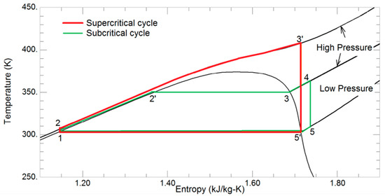
Figure 1.
Typical subcritical and supercritical cycles in temperature-entropy diagram.
The analysis and performance evaluation of supercritical ORC cycles mainly focused on fluid selections [6,15,19,20], design and optimization [15,21,22,23,24,25,26,27]. Although steady-state models of ORC-WHR systems are necessary for the preliminary analyses as discussed above, they cannot be used either for performance evaluation in transient conditions or control system simulations. Therefore the dynamic model of the ORC-WHR system is proposed by the authors in [28]. Since the dynamics of the overall ORC systems evolve around the evaporator, the critical component of the system, the model is developed using conventional finite volume (FV) method. In this method, the evaporator is discretized into several finite segments and heat transfer equations for each segment are solved numerically. The FV is a robust and accurate method which is commonly used as can be seen in [12,29,30]. Despite the fact that the FV model is accurate and able to capture the variable thermo-physical properties of the supercritical fluids as described in [31], it is very time intensive for computation and this limits its real-time applications. To eliminate the limitation, a novel fuzzy-based dynamic evaporator mode is developed and presented in this paper. The knowledge and transient response of the evaporator and the ORC system under variable heat input conditions analyzed using the FV model is used to predict the thermal inertia of the fuzzy model. Other components of the cycle are also developed and then integrated with the novel fuzzy-based dynamic evaporator model to investigate the performance of the system under a variable heat source. The detailed performance of the evaporator model, which is based on fuzzy and the complete ORC-based WHR system are validated and presented in this research.
This paper is organized as follows; the next section presents the system description of the ORC-WHR considered in this research. Section 3 presents the individual components models including FV and fuzzy-based evaporator, model validations and integrations. The performance of the dynamic system is evaluated and discussed in Section 4. Finally, the research findings and conclusions are presented in Section 5.
2. ORC-WHR System
The ORC-WHR system studied consists of a pump, an evaporator, an expander couple with a generator, a condenser, and an accumulator, as shown in Figure 2. Additionally, a valve in dynamic conditions is used to manage the system start-up and shut-down procedures. The ORC is similar to the conventional steam Rankine cycle but uses organic fluids instead of water as a working fluid. The organic fluid has desirable thermo-physical properties, such as low boiling point and high vapor pressure, that are suitable for low to medium grade heat recovery applications with a output capacity from a few kilowatts to a couple of hundred kilowatts [8,29,32,33]. In this research, R134a was chosen as the working fluid as it has advantages such as availability, wide commercial use, low critical temperature, high auto-ignition temperature, and suitability for low grade heat recovery applications. The thermo-physical properties of R134a are shown in Table 1. The working fluid of the ORC is pumped to the evaporator and heated up by a heat source to its evaporating point, e.g., a pressurized hot water, and then expanded in the expander to drive a coupled generator. The excess heat contained in the working fluid is released at the condenser, and then the cold fluid is sent back to the accumulator and completes the cycle. The ORC-WHR system will be simulated at a pressure of 6 MPa, which is a supercritical pressure that is much higher than the working fluid used in most thermal cycles.
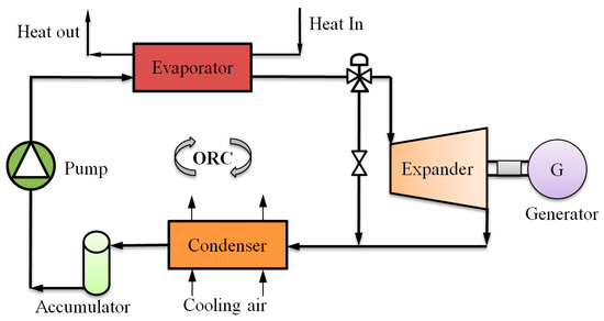
Figure 2.
Components of a typical organic Rankine cycle-based waste heat recovery (ORC-WHR) system.

Table 1.
Properties of R134a.
3. Model Development
The components of the ORC-WHR system described in the previous section are modelled and integrated in this section. The modelling of the valve, however, is disregarded due to that fact that the start-up and shut-down procedures are not covered in this paper.
3.1. Evaporator Model
The evaporator is a critical component of the ORC system since effective heat transfer from this component influences the thermal efficiency of the system. Also, due to the transient nature of heat sources from industry and automotive sectors, the evaporator is primarily treated as a source of thermal inertia in the system. Several heat exchangers can be employed as the evaporator in WHR systems. These are the finned tube, the shell and tube and the plate heat exchangers, etc. Plate heat exchangers are highly recommended in this application because they are compact and have a large area, which aims to recover the most possible quantity of heat from the main heat source [5]. Other advantages of plate heat exchangers are also a minimum risk of internal leakage, minimum pressure drop, and less complexity in maintenance [34].
3.1.1. Finite Volume Model
The FV method is used to develop the dynamic model of the evaporator where the heat exchanger is discretized into a finite number of segments along the direction of the flow (See Figure 3). The number of segments, N on both sides and wall of the heat exchanger, is the same. In the numerical model, the input and output parameters of the working fluid and the heat source are imposed on the inlet and outlet sides of each segment as shown in Figure 3. These parameters are stored at locations called nodes. The number of nodes n is therefore, n = N + 1.
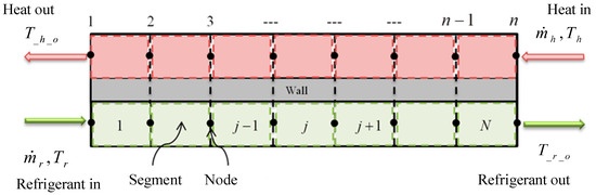
Figure 3.
Finite volume (FV) discretization of evaporator.
Below assumptions are used to develop the FV evaporator model:
- The heat exchanger model is assumed to be one-dimensional, and the heat transfer to surrounding environment is neglected.
- The momentum conservation is not considered in the model and the pressure variation within the model is assumed to be negligible.
- The heat transfer between the heat source and the refrigerant takes place not by conduction but by convection.
- Heat exchanger wall is uniformly built, and thermo-physical properties are assumed to be constant.
- Thermo-physical properties of refrigerant and heat source fluid for each discrete segment are constant.
All these assumptions are commonly used to simplify the modelling effort and reduce the computational time, which can be seen in the literature [12,22,29,35]. Details of mass and energy conservation equations of the FV method are completely discussed by the authors in [28].
Solution Methodology
In the FV approach, the heat source and the refrigerant outlet conditions have been initially guessed. Using the initial and inlet conditions, the simultaneous first-order differential equations for the wall, the refrigerant, and heat source of the FV model described in [28] are solved accordingly. The time-dependent terms in the governing equations are integrated using the Euler explicit method. This method is one of the known approaches used for the solution of time-dependent ordinary or partial differential equations. In this approach, the numerical approximation of the time-dependent term at the next time step is calculated from the state of the term at the current step. The numerical discretization of the FV evaporator model in the time domain can be represented as follows:
where and are the convective heat transfer coefficients (kW/m2K) of the heat source fluid and refrigerant with the wall; and (kJ/kgK) are the specific heat capacity of the heat source and heat exchanger wall, respectively. (kg/s), (K) and (KJ/kg K) are the mass flow rate, temperature and enthalpy of the refrigerant; , and are the mass flow rate, temperature of heat source and temperature of wall, respectively.
Time-Step Determination
In order to achieve a stable solution of the discretized Equations (1)–(3), a correlation to calculate the time step can be derived from the equations that contain the variables of interest and . To obtain a stable solution, the coefficients of and variables in Equations (1)–(3) should be greater than zero. Therefore, from Equation (1), it can be written as follows:
Similarly, from Equation (2), this can be written as,
The evaporator model time step should be the minimum of the two values in Equations (4) and (5) which can be represented by Equation (6). The minimum time step in the discretized equations can guarantee a stable solution in the numerical model.
Simulation Procedure
The dynamic evaporator model consists of two parts as shown in Figure 4. They are the steady state part and the dynamic part. In the steady state calculation, the model is converged to the steady state condition before applying any transient inputs to the model. This convergence reduces the effect of initial assumptions to the accuracy when the model is simulated in the transient conditions. The steps involved in the solution of discretized Equations (1)–(3) are as follows:
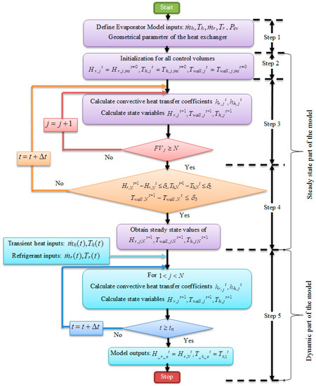
Figure 4.
Program flow-chart of the dynamic evaporator model.
Step 1: Define the geometrical parameters, heat source fluid and refrigerant inputs and a discrete time step of the evaporator including the number of segments and nodes of the model. REFPROP [36] database has been utilized to obtain the thermo-physical properties of the refrigerant and the heat source fluid during the simulation.
Step 2: The second phase is the initialization which is an important issue for every dynamic system in numerical methods. Given the steady inputs, the unknown parameters of Equations (1)–(3) are initialized by assuming the appropriate values at as follows:
From the refrigerant’s initial enthalpy distribution, the temperature of the segment can be retrieved as follows:
The initial temperatures of the refrigerant and the heat source fluid are used to define the initial temperature of the wall as follows:
The initial temperatures of the fluids and wall mass are assigned equally to all segments to have an initial temperature distribution for the model. This initial distribution does not necessarily have to be accurate since they serve only as a starting point for the simulation. Once all the parameters of the current time are available, the solution of the discretized Equations (1)–(3) can be started.
Step 3: Based on the enthalpy, temperature distribution and the initial inputs condition at the previous step, this step retrieves thermodynamic properties from REFPROP and calculates the convective heat transfer coefficients of the heat source fluid and refrigerant at , respectively. Thermo-physical properties and the local temperature are considered in calculating the convective heat transfer coefficients in Equations (1)–(3), using the Nusselt number () and Reynolds number () correlations in Equation (10). The specific Nusselt number correlations for the heat source fluid and the refrigerant are discussed by the authors and can be found in [28].
where , , and are the hydraulic diameter of the plate heat exchanger, the density of the fluid in (kg/m3) and the viscosity in (Pa.s) and the velocity of the fluids (m/s), respectively.
Within this simulation step, the enthalpy, heat source temperature and wall temperature for the next time step are calculated using Equations (1)–(3). This simulation step is repeated until the calculation reaches to the final segment of the model.
Step 4: At this step of the simulation, the Nth values of the refrigerant enthalpy, heat source temperature and wall temperature at and at are compared. If the differences between consecutive values are less than the predefined steady-state convergence values of and , which is 0.0001, the solution is said to have achieved the steady state condition. Otherwise, steps 1–3 are repeated until the steady state condition is reached. At the end of Step 4, the initial distribution of the refrigerant enthalpy, the heat source temperature, and the wall temperature are all converged to the actual value and the effect of the initial assumptions are now completely vanished.
Step 5: The dynamic part of the model is started at the end of the steady state part as depicted in Figure 4. The transient inputs to the model are introduced at this step. At a discrete time-step and model time , the calculation of the state variables is continued along the segments . At the end of each time step, the values of the state variables are stored in the MATLAB workspace. The dynamic simulation is continued until it reaches the final predefined model time .
Numerical Issues
The discrete time step in Equation (6) depends on the mass flow rate of each fluid, the density of each fluid and the volume of each discrete segment. Since the mass flow rate and density of the fluids are time dependent variables and can vary during the simulation, the discrete time step should also vary according to Equation (6). Calculating a variable time step during the simulation will make the computation process more complicated and time-consuming. Moreover, this process has a limitation in a real-time application as the temperature at the evaporator inlet, and therefore the properties of the fluid is unknown and cannot be predicted in advance. Therefore, instead of defining a variable time step, a fixed time step is used based on the maximum and minimum temperature and flow rate ranges used in the simulation. In this process, the discrete time step is set to 0.1 s in the simulation, which is selected using Equation (6) that can guarantee a stable solution of the discretized Equations (1)–(3).
In the FV technique, the number of finite cells is also an important issue that influences the accuracy as well as the time requirement of the simulation. To evaluate the error of the calculation, the outputs of the model at different numbers of segments (10, 20 and 50) are compared with that of a 100 segments model, which is taken as the reference value. The computation errors correspond to 10, 20, and 50 segments model for the prediction of the refrigerant enthalpy are approximately 7%, 3.1%, and 0.8%, respectively. On the contrary, the calculation error for the outlet temperature of the heat source is below 1% for all number of segments in the simulation. It is as expected that the higher accuracy is achieved with the higher number of segments. However, this higher number of segments leads to an extensive computation time. Therefore, in this simulation the number of segment is set to 20, as it is a good trade-off between the model accuracy and the simulation time.
Transient Response Simulation
To evaluate the performance of the evaporator model in transient situations, three different tests have been carried out. The step change to the inlet temperature and mass flow rate of the heat source are the first and second test. Finally, the step change in the mass flow rate of the refrigerant is also investigated in this section.
Figure 5 depicts the evaporator model response to a step change in the heat source inlet temperature. The step magnitude of 48 K at t = 150 s, which is arbitrarily chosen, is applied to the inlet temperature of the heat source. To discard the effects of the assumptions initially considered, the model is converged into the steady state condition before the step change occurred at t = 150 s. The other variables at the inlet are kept constant during this transient response test, and the calculation is continued until the steady state condition is obtained.
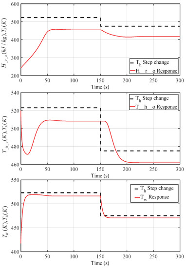
Figure 5.
Response of with respect to step change.
To investigate the effect of a mass flow rate transient on the model outputs, a step change of 0.2 kg/s to the mass flow rate of the heat source is imposed at t = 150 s. Figure 6 shows the responses of refrigerant enthalpy, heat source temperature and wall temperature to the step change. Similarly, a step change of 0.15 kg/s to the refrigerant flow rate is also imposed and the transient responses of the model are illustrated in Figure 7. The outlet variable responses due to the step changes in the heat source and refrigerant inputs indicate that the proposed model is stable and can be used to simulate the transient behavior of the inlet conditions.
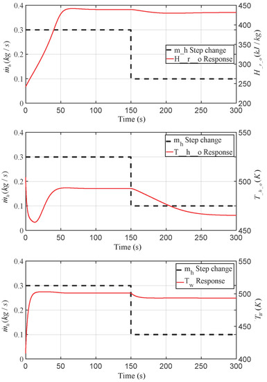
Figure 6.
Response of with respect to step change.
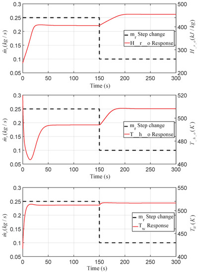
Figure 7.
Response of with respect to step change.
The response time of the evaporator model to different transient steps is shown in Table 2. The response time is a time that is required for a time-dependent variable to reach from one steady state value to 63% of the final steady state value [37]. The state values of the evaporator model at the 63% response time are also shown in Table 2. It can be seen from Figure 5, Figure 6 and Figure 7 and Table 2 that the ideal response time is different with respect to different step changes, which is as expected since the modification in one inlet condition will change all outlet conditions according to their nonlinear relationship as represented by Equations (1)–(3). The results from the transient response analysis indicate that the behavior of the evaporator model is satisfactory and therefore can be used in the simulation of the system dynamics.
Table 2.
Ideal response time of finite volume (FV) evaporator model outputs.
Simulation Time Constraint in Dynamic Scenario
There are several factors that can increase the simulation time of the evaporator model in both the steady state and dynamic conditions. The first factor is the discrete time step and the second factor contributes to the higher simulation time is the number of segments of the model.
In the dynamic situation, since the model initially needs to converge into a steady state condition before applying the transient heat source, the simulation time of the model can be evaluated by combining the time required for both conditions. The simulation time of the evaporator model with the random transient heat source in Figure 8 is presented in Table 3. It can be concluded from Table 3 that despite the total simulated run-time of the system being kept the same, the actual computing time of the simulation is increased with the number of segments. The model with this higher simulation time will show poor performance in real-time control applications. Therefore, to reduce the simulation time, a second approach to develop the evaporator model using the fuzzy technique is proposed in the next section.
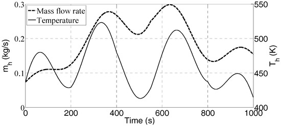
Figure 8.
Heat source mass flow rate and temperature [28].
Table 3.
Computation time for a transient heat source simulation.
3.1.2. Fuzzy Based Dynamic Evaporator Model
Almost all dynamic systems in practical applications are nonlinear. Modelling of those systems cannot be represented by simple linear differential equations. It requires a set of high order nonlinear equations which make the whole system too complex to be used in a control system. In the WHR system, the evaporator operating under variable heat source is a nonlinear. Nonlinear models of the evaporator in a WHR system have been developed and are shown in several reports [30,38]. However, even with the simplified assumption and model order reduction made for the evaporator, high nonlinearity still makes the system complex and time-consuming for the simulation [39]. The simplified 1D FV model of the evaporator developed in this research is also a nonlinear model and required extensive time in simulations as shown in Table 3. The nonlinearity of the model comes from the state variables, which are the functions of the thermodynamic properties and input conditions according to Equations (1)–(3). For this reason, this section presents a dynamic model of the evaporator based on fuzzy logic. The fuzzy logic is a multivalued logical system that provides the value of an unknown output by attaching the degree of known input and output of the system [40]. The fuzzy logic concept can be used to develop a model of a nonlinear system which does not require a set of complex mathematical equations. Therefore, it requires less resource and saves substantial computation time.
The design of the dynamic fuzzy-based evaporator model is similar to that of the FV model. The evaporator model has three inputs (refrigerant mass flow rate , heat source mass flow rate and heat source temperature ) and two outputs (outlet temperature of the refrigerant and outlet temperature of heat source ).
The dynamic fuzzy model is composed of two parts: the fuzzy inference system and the thermal inertia of the system as shown in Figure 9. The outputs of the fuzzy inference system, and , are fed to the thermal inertia calculation block. The dynamic model outputs, and , are then obtained from the thermal inertia block.
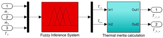
Figure 9.
Fuzzy-based dynamic evaporator model.
Based on the data available from the FV dynamic model, the range of the inputs and output parameters are determined and adjusted from the experience about the system of the designer as follows: [0.01 (kg/s), 0.25 (kg/s)], [0.05 (kg/s), 0.300 (kg/s)], [400 (K), 523 (K)], [364.5 (K), 470 (K)] and [285 (K), 595 (K)], respectively. To obtain a high efficiency of the fuzzy inference system, the input and output variables are normalized in between 0 and 1 as illustrated in Figure 10 and Figure 11. The actual crisp values of the model parameters are calculated from the normalized values as follows:
where , , , and are the normalized values of their corresponding variables.
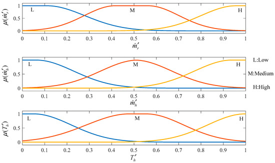
Figure 10.
Normalized membership functions of input variables.
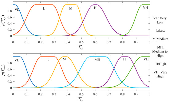
Figure 11.
Normalized membership functions of output variables.
The fuzzy-based model input and output ranges must be classified into different linguistic levels, which are called membership functions. The linguistic level assigned to the input variables , , are: L: Low; M: Medium and H: High. The output variable is designed by five membership functions: VL: Very Low; L: Low; M: Medium; H: High and VH: Very High; and has one additional membership function than that is Medium to High, MH. The numbers of membership functions were selected in a way so that they can capture the transient nature of the evaporator at an accuracy over 90%. All the inputs-outputs variables and their membership functions are shown in Figure 10 and Figure 11.
Once the membership functions of the input and output variables are all set, the next step is to define the rules and create a logical relationship among the membership functions of the model inputs and the model outputs. The fuzzy rules are established using the abovementioned sets of the input and output variables as follows:
where , is the number of fuzzy rules, , , , , are the th fuzzy sets of the input and output variables of the fuzzy system.
The rules of the fuzzy model are generally defined from the knowledge of characteristics of a system. In this dynamic model, rules are established from the intuition and knowledge of the evaporator used in this paper. The rules of the fuzzy dynamic model are presented in Table 4. Overall mapping of the input parameters to the outputs represented by the fuzzy rules can be plotted as 3D surfaces. The fuzzy surfaces of the evaporator and heat source outlet temperature are shown in Figure 12 and Figure 13.
Table 4.
Fuzzy rules of dynamic model of the evaporator. VL: Very Low; L: Low; M: Medium; MH: Medium to High; H: High and VH: Very High.
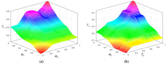
Figure 12.
Fuzzy surface of evaporator outlet temperature with respect to and (a) and (b).
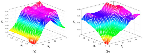
Figure 13.
Fuzzy surface of heat source outlet temperature with respect to and (a) and (b).
Among different fuzzy reasoning methods, the MAX-MIN method [41] is utilized to obtain the output from the present input and the inference rules. For a given particular input fuzzy set in , the output fuzzy set in for is computed through the inference system is as follows:
The output membership functions for is calculated similarly. In this research, the membership functions used for the dynamic evaporator model are Gaussian type denoted by in Figure 10 and Figure 11.
In addition, among different methods of defuzzifications, the centroid defuzzification method [42] is used in this model to convert the aggregated fuzzy set to a crisp output value from the fuzzy set . This work computes the weighted average of the membership function or the center of gravity (COG) of the area bounded by the membership function curves [43]:
The crisp value of and were calculated utilizing the above equation. The crisp values of the fuzzy inference systems are fed to the thermal inertia block to obtain the final output values of the fuzzy-based model.
The thermal inertia of the fluids in the evaporator is dependent on the fluid’s properties such as specific heat capacity, thermal conductivity, the volume flow rate of the fluid, etc., and the geometrical dimension and thermal properties of the evaporator wall. The thermal inertia of the fluid streams can be expressed by a time delay with respect to a change of the fluids temperature. The knowledge of the transient behavior of the evaporator model in the dynamic condition is used to define the time delay for the refrigerant and heat source temperature in the fuzzy-based model. The following transfer functions represent the time delay of the model.
Transfer function for the refrigerant’s outlet temperature delay is as follows:
The transfer function for the heat source outlet temperature delay is as follows:
The numerator and denominator values of the two transfer functions were adjusted according to the response of the evaporator against the transient heat inputs studied in this research.
3.1.3. Evaporator Model Validation
The fuzzy-based dynamic model is validated with the data available from the dynamic FV model of the evaporator. The outputs of the fuzzy model with respect to the FV model are shown in Figure 14 and Figure 15. It can be observed from these figures that the fuzzy-based model can predict the evaporator outputs effectively in the dynamic condition. The data fitness values of 90.32% and 91.24% are obtained for the outputs of and , respectively. The RMSE (Root Mean Squared Error) and MAPE (Mean Absolute Percentage Error) of the fuzzy model outputs with respect to the validation data is shown in Table 5. The fuzzy model can predict the outputs with a RMSE of 1.10 K for and 3.09 K for , which gives a MAPE of 0.19% and 0.58%, respectively. Moreover, the time used for the simulation of the random heat source in the fuzzy-based model is 5.19 s, compared to 3820.6 s of the FV model. This implies that the fuzzy model with an accuracy of above 90% is 736.15 times faster than that of the FV model. These validation numbers indicate that the fuzzy logic concept is suitable to develop the dynamic evaporator model in the WHR system.
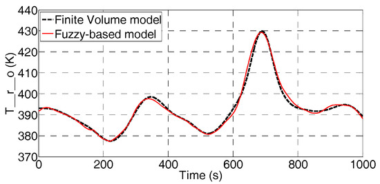
Figure 14.
Comparison of evaporator outlet temperature of fuzzy-based and FV models.
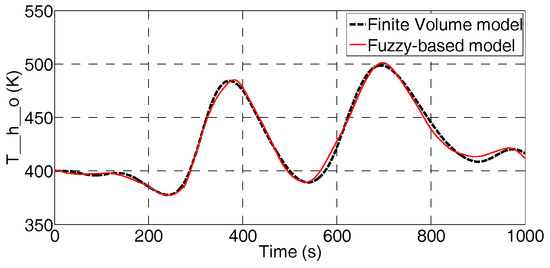
Figure 15.
Comparison of heat source outlet temperature of fuzzy-based and FV models.
Table 5.
Performance of fuzzy-based dynamic evaporator model.
3.2. Other Component Models
3.2.1. Pump Model
The pump used in this research is a volumetric diaphragm pump [44], which is a positive displacement machine. The response of such pumps are much faster than the response of the heat exchanger in the ORC-WHR system [45]. For this reason, complicated dynamics of the pump are not necessary for the simulation of the WHR dynamics. A constant efficiency and the performance curve of the pump provided by the manufacturer can be used for the development of the pump model. The characteristic of the diaphragm pump is that the mass flow rate is proportional to the speed of the pump [14,46]. The performance curve of the pump can be used to derive the relationship between the speed of the pump and the refrigerant mass flow rate as follows [38,44]:
where is the mass flow rate of the pump in kg/s and is the corresponding pump speed in RPM.
The specific work input as a function of the pump’s pressure and enthalpy difference can be calculated as follows:
where is the specific volume in m3/kg; and are the pump inlet and outlet enthalpy in kJ/kg, respectively; is the pump work in kW; is the mechanical efficiency of the high pressure diaphragm pump; and are the inlet and outlet pressures of the pump in kPa, respectively.
3.2.2. Expander Model
An expander in a WHR system is generally one of two types: volumetric expander i.e., piston, scroll, etc. and a turbo-machinery type i.e., turbines. The time response of both volumetric and turbo-machinery expanders are much faster compared with the evaporator in the WHR system. Therefore, similarly with the pump, the dynamics of the expander is unnecessary in the simulation of WHR system. The steady state thermodynamic model of the expander is used for the simulation of the expander in this investigation. The specific work output of the expander is calculated as follows:
where is the expander work output, is the refrigerant mass flow rate through the expander; and are the expander inlet and outlet enthalpy, respectively; is the expander efficiency.
3.2.3. Condenser Model
The dynamics of the WHR system are mostly formed by the dynamic behaviors of both evaporator and condenser. Therefore, the dynamic evaporator and condenser models were taken into account in the simulation of the WHR dynamics as shown in several reports [30,38,45]. Although both the evaporator and condenser have significant effects on the operating parameters of the ORC-WHR system, the dynamic model of the evaporator is of greater importance than that of the condenser. This is, especially at supercritical pressure, because of the unpredictable heat transfer mechanism at the evaporator. Therefore, a thermodynamic model of the condenser based on the state enthalpy is adequate to represent the condenser as follows:
where is the condenser cooling power in kW, is the mass flow rate of refrigerant through the condenser and is the enthalpy at the condenser outlet.
3.2.4. Accumulator Model
To absorb the organic fluid fluctuations and make sure that there is liquid at the inlet of the pump, an accumulator is used between the pump inlet and the condenser outlet. The organic fluid level in the cycle is represented by following conservation equations [38,47].
where is the relative liquid refrigerant level in the accumulator, is the liquid refrigerant density, is the volume of the accumulator tank, is the mass flow rate of the refrigerant at the accumulator inlet, and is the mass flow rate of the refrigerant at the accumulator outlet. and are the enthalpy of the refrigerant at the inlet and outlet of the accumulator, respectively.
3.3. Model Integration
The component models of the supercritical ORC-WHR system described in Section 3.1 and Section 3.2 are integrated to form an overall system dynamic model. The overall model parameters are given in Table 6. The inputs and outputs of each component in the dynamic model are linked according to the rationalities described as follows:
Table 6.
The organic Rankine cycle (ORC) model parameters.
- The pump delivers the refrigerant mass flow rate at a proportion to the speed of the pump. Given the inlet and outlet pressure, the electrical power requirement to drive the pump and the temperature of the fluid at the outlet can be calculated.
- There is no enthalpy loss in between the pump and the evaporator. The heat recovery in the evaporator is a function of the inlet flow conditions and working pressure of the fluids.
- The expander can rotate freely without imposing any speed constraint. The amount of work output is a function of the enthalpy at the inlet and outlet of the expander.
- Provided the condenser outlet temperature is constant, the model calculates the required cooling power to achieve the desired temperature at the outlet.
- Given the inlet conditions and mass of the fluid, the accumulator maintains the outlet enthalpy and fluid level.
The pressure loss because of piping work between the evaporator and the expander in the overall WHR system is modelled using the Darcy–Weisbach pressure drop correlation as follows:
where is the Darcy friction factor, is the density of the pipe, is the length of the pipe, is the velocity of the fluid, and is the hydraulic diameter of the pipe.
The friction factor is calculated using the Haaland equation [48] as follows:
where is the absolute roughness, and is the relative roughness of the pipe.
4. Results and Analysis
The performance of the fuzzy-based overall model compared to the FV-based overall model in predicting the pressure at the expander inlet, the expander work output and the cycle efficiency is presented in this section. The simulation was conducted with the same input conditions as used for the fuzzy model validation in Section 3.1.3.
The pressure at the expander inlet after considering the loss is shown in Figure 16. It can be seen from this figure that the expander inlet pressure for both cases of the overall model are similar except for some small deviations around time 200 s, 400 s, and 800 s. These deviations of pressure are caused by the predicting error of the evaporator outlet temperature in the fuzzy domain, which is one of the functions of the pressure loss correlation used in Equation (27). However, the error in the fuzzy-based evaporator model predicting the expander inlet pressure was only 0.001%, which is shown in Table 7. The performance of the overall models for the prediction of expander work output is shown in Figure 17. The MAPE of the fuzzy-based overall model for the work output is at 3.11% (see Table 7). This discrepancy between the fuzzy-based and FV-based overall model is due to the fact the output from the evaporator is also one of the inputs of the expander, thus the error associated in the evaporator model will lead to the error in the prediction of expander output.
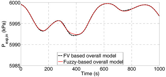
Figure 16.
Prediction of expander inlet pressure with the fuzzy and FV evaporator-based overall models.
Table 7.
Mean values of operating parameters with respect to random inputs.
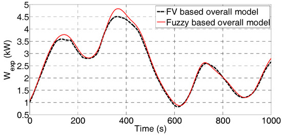
Figure 17.
Prediction of expander power output with the fuzzy and FV evaporator-based overall models.
The cycle efficiency of the ORC-WHR system is represented by and can be written as:
where is the net output work and is heat recovered at the evaporator.
The evaporator heat input in Equation (29) can be calculated from the mass flow rate and temperature of the refrigerant at the inlet and outlet of the fuzzy-based evaporator model.
The cycle efficiency of the fuzzy-based overall model in comparison to the FV-based model for the entire operation period is shown in Figure 18. Since the simulation in this paper was carried out with a random heat source and refrigerant input to the system, the efficiency was varied according to the combination of the heat source inputs, refrigerant inputs, and expander output, as shown in Figure 18. The cycle efficiency of the ORC-WHR system presented in this paper was neither controlled nor optimized during the simulation. Therefore, the outputs are followed according to the inputs only. It can be noticed that the maximum efficiency obtained in the simulation of the FV-based and fuzzy-based overall models are 13.36% and 12.86%, respectively. The FV-based overall model led to an average cycle efficiency of 9.78%, while the fuzzy-based overall model led to 9.42%. Since the cycle efficiency is a function of the temperature at the evaporator outlet, the error in the temperature calculation of the fuzzy-based evaporator model contributed to the efficiency calculation which can be seen in Figure 18 and Table 7. The results presented in this figure provide a MAPE error of less than 4% in predicting the cycle efficiency of the system using the fuzzy-based overall model compared to the FV model. Moreover, it can also be seen from Figure 18 that the efficiency prediction difference between the FV-based and the fuzzy-based model is always less than around 0.5%. The results indicate that the fuzzy-based evaporator model can be integrated with other components to predict the efficiency of the ORC-WHR system in dynamic conditions.
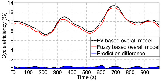
Figure 18.
Cycle efficiency with respect to random inputs.
5. Conclusions
This paper presents the modelling of a dynamic ORC-WHR system using a well-known FV technique and a novel fuzzy method. The performance analysis of the dynamic model regarding individual components and overall model is presented.
Since the evaporator was the focus of the research, the dynamic model of this component was initially developed using the conventional FV method. The detailed performance analysis of the model regarding the transient response was carried out. Results show that the model is sufficiently stable and responses to the transient inputs are satisfactory. This implies that the model was robustly built to be used in the dynamic scenario of the WHR system. However, because of the high computation time of this method, a second model of the evaporator based on the fuzzy inference system was developed. Useful information about the evaporator in the dynamic condition such as transient responses, input-output ranges, thermal inertia, etc. obtained from the FV model were used to develop the fuzzy model. The outputs of the fuzzy-based model were validated with that of the FV model. The results from the validation indicate that the fuzzy inference system can be used to predict the evaporator outputs in the dynamic situation.
A pump, an expander, a condenser, and an accumulator were added to the proposed dynamic model of the evaporator to provide a complete overall model of the dynamic ORC-WHR system. The performance analysis of the overall model with the integration of the fuzzy evaporator model shows that the model was able to predict the pressure at the inlet of the expander, the expander output, and the cycle efficiency accurately. This shows that the fuzzy-based evaporator model in the WHR system can be used to simulate the system performance and to develop control strategies under transient heat input conditions.
Acknowledgments
This publication was supported by the Engineering and Physical Sciences Research Council (EPSRC, EP/P004636/1, UK).
Author Contributions
Jahedul Islam Chowdhury developed the methods, codes, carried out the simulation work, analyzed the results and wrote the manuscript. Bao Kha Nguyen helped with the developing programming codes and reviewing the paper. David Thornhill contributed in analyzing the results. Yukun Hu helped with the structuring, writing the paper and analyzing the results. Payam Soulatiantork helped with the writing and reviewing the paper. Nazmiye Balta-Ozkan and Liz Varga provided instructions to improve the analysis quality, reviewed the paper and provided valuable suggestions. All authors agreed about the contents and approved the manuscript for submission.
Conflicts of Interest
The authors declare no conflict of interest.
Nomenclature
| Heat transfer area, m2 | |
| Specific heat capacity, kJ/kgK | |
| Hydraulic diameter, m | |
| Friction factor | |
| Specific enthalpy, kJ/kg | |
| Heat transfer coefficient, kW/m2K | |
| Thermal conductivity, W/mK | |
| Length, m | |
| Mass flow rate, kg/s | |
| Rotational speed of pump, RPM | |
| Number of segments | |
| Node | |
| Nusselt number | |
| Pressure, kPa | |
| Q | Heat input, kW |
| Reynolds number | |
| s | Second |
| Temperature, K | |
| Volume, m3 | |
| v | Velocity, m/s |
| Power output, kW or plate width, m | |
| Pressure loss, kPa | |
| Time step | |
| Efficiency, % | |
| Dynamic viscosity, Pa.s or Membership functions | |
| Density, kg/m3 | |
| Specific volume, m3/kg | |
| Absolute roughness, m | |
| Response time, s | |
| Convergence coefficient | |
| Relative level | |
| Subscripts | |
| ac | accumulator |
| c | cold |
| cy | cycle |
| con | condenser |
| ev | evaporator |
| exp | expander |
| h | heat source |
| i | inlet |
| j | segments notation |
| l | liquid |
| max | maximum |
| min | minimum |
| o | outlet |
| p | pump, pipe |
| pl | plate |
| r | refrigerant |
| t | time |
References
- IPCC Climate Change 2014: Mitigation of Climate Change. Available online: https://www.ipcc.ch/report/ar5/wg3/ (accessed on 1 June 2016).
- Boretti, A. Recovery of exhaust and coolant heat with R245fa organic Rankine cycles in a hybrid passenger car with a naturally aspirated gasoline engine. Appl. Therm. Eng. 2012, 36, 73–77. [Google Scholar] [CrossRef]
- Johansson, M.T.; Söderström, M. Electricity generation from low-temperature industrial excess heat—An opportunity for the steel industry. Energy Effic. 2014, 7, 203–215. [Google Scholar] [CrossRef]
- Gheith, R.; Aloui, F.; Ben Nasrallah, S. Determination of adequate regenerator for a Gamma-type Stirling engine. Appl. Energy 2015, 139, 272–280. [Google Scholar] [CrossRef]
- Ziviani, D.; Beyene, A.; Venturini, M. Advances and challenges in ORC systems modeling for low grade thermal energy recovery. Appl. Energy 2014, 121, 79–95. [Google Scholar] [CrossRef]
- Gao, H.; Liu, C.; He, C.; Xu, X.; Wu, S.; Li, Y. Performance analysis and working fluid selection of a supercritical organic rankine cycle for low grade waste heat recovery. Energies 2012, 5, 3233–3247. [Google Scholar] [CrossRef]
- Shu, G.; Yu, G.; Tian, H.; Wei, H.; Liang, X. A Multi-Approach Evaluation System (MA-ES) of Organic Rankine Cycles (ORC) used in waste heat utilization. Appl. Energy 2014, 132, 325–338. [Google Scholar] [CrossRef]
- Zhang, J.; Zhou, Y.; Li, Y.; Hou, G.; Fang, F. Generalized predictive control applied in waste heat recovery power plants. Appl. Energy 2013, 102, 320–326. [Google Scholar] [CrossRef]
- Tian, H.; Shu, G.; Wei, H.; Liang, X.; Liu, L. Fluids and parameters optimization for the organic Rankine cycles (ORCs) used in exhaust heat recovery of Internal Combustion Engine (ICE). Energy 2012, 47, 125–136. [Google Scholar] [CrossRef]
- Wang, Z.Q.; Zhou, N.J.; Guo, J.; Wang, X.Y. Fluid selection and parametric optimization of organic Rankine cycle using low temperature waste heat. Energy 2012, 40, 107–115. [Google Scholar] [CrossRef]
- Sun, J.; Li, W. Operation optimization of an organic rankine cycle (ORC) heat recovery power plant. Appl. Therm. Eng. 2011, 31, 2032–2041. [Google Scholar] [CrossRef]
- Quoilin, S.; Aumann, R.; Grill, A.; Schuster, A.; Lemort, V.; Spliethoff, H. Dynamic modeling and optimal control strategy of waste heat recovery Organic Rankine Cycles. Appl. Energy 2011, 88, 2183–2190. [Google Scholar] [CrossRef]
- Hou, G.; Sun, R.; Hu, G.; Zhang, J. Supervisory predictive control of evaporator in Organic Rankine Cycle (ORC) system for waste heat recovery. In Proceedings of the 2011 International Conference on Advanced Mechatronic Systems, Zhengzhou, China, 11–13 August 2011. [Google Scholar]
- Zhang, J.; Zhang, W.; Hou, G.; Fang, F. Dynamic modeling and multivariable control of organic Rankine cycles in waste heat utilizing processes. Comput. Math. Appl. 2012, 64, 908–921. [Google Scholar] [CrossRef]
- Schuster, A.; Karellas, S.; Aumann, R. Efficiency optimization potential in supercritical Organic Rankine Cycles. Energy 2010, 35, 1033–1039. [Google Scholar] [CrossRef]
- Glover, S.; Douglas, R.; Glover, L.; McCullough, G. Preliminary analysis of organic Rankine cycles to improve vehicle efficiency. Proc. Inst. Mech. Eng. Part D J. Automob. Eng. 2014, 228, 1142–1153. [Google Scholar] [CrossRef]
- Lecompte, S.; Huisseune, H.; van den Broek, M.; De Paepe, M. Methodical thermodynamic analysis and regression models of organic Rankine cycle architectures for waste heat recovery. Energy 2015, 87, 60–76. [Google Scholar] [CrossRef]
- Chen, H.; Goswami, D.Y.; Rahman, M.M.; Stefanakos, E.K. A supercritical Rankine cycle using zeotropic mixture working fluids for the conversion of low-grade heat into power. Energy 2011, 36, 549–555. [Google Scholar] [CrossRef]
- Dai, X.; Shi, L.; An, Q.; Qian, W. Screening of hydrocarbons as supercritical ORCs working fluids by thermal stability. Energy Convers. Manag. 2016, 126, 632–637. [Google Scholar] [CrossRef]
- Glover, S.; Douglas, R.; Glover, L.; Mccullough, G.; Mckenna, S. Automotive waste heat recovery: working fluid selection and related boundary conditions. Int. J. Automot. Technol. 2015, 16, 399–409. [Google Scholar] [CrossRef]
- Glover, S.; Douglas, R.; De Rosa, M.; Zhang, X.; Glover, L. Simulation of a multiple heat source supercritical ORC (Organic Rankine Cycle) for vehicle waste heat recovery. Energy 2015, 93, 1568–1580. [Google Scholar] [CrossRef]
- Karellas, S.; Schuster, A.; Leontaritis, A.D. Influence of supercritical ORC parameters on plate heat exchanger design. Appl. Therm. Eng. 2012, 33–34, 70–76. [Google Scholar] [CrossRef]
- Yağli, H.; Koç, Y.; Koç, A.; Görgülü, A.; Tandiroğlu, A. Parametric optimization and exergetic analysis comparison of subcritical and supercritical organic Rankine cycle (ORC) for biogas fuelled combined heat and power (CHP) engine exhaust gas waste heat. Energy 2016, 111, 923–932. [Google Scholar] [CrossRef]
- Le, V.L.; Feidt, M.; Kheiri, A.; Pelloux-Prayer, S. Performance optimization of low-temperature power generation by supercritical ORCs (organic Rankine cycles) using low GWP (global warming potential) working fluids. Energy 2014, 67, 513–526. [Google Scholar] [CrossRef]
- Chowdhury, J.I.; Nguyen, B.K.; Thornhill, D. Investigation of waste heat recovery system at supercritical conditions with vehicle drive cycles. J. Mech. Sci. Technol. 2017, 31, 923–936. [Google Scholar] [CrossRef]
- Braimakis, K.; Preißinger, M.; Brüggemann, D.; Karellas, S.; Panopoulos, K. Low grade waste heat recovery with subcritical and supercritical Organic Rankine Cycle based on natural refrigerants and their binary mixtures. Energy 2015, 88, 80–92. [Google Scholar] [CrossRef]
- Chowdhury, J.I.; Soulatiantork, P.; Nguyen, B.K. Simulation of Waste Heat Recovery System with Fuzzy Based Evaporator Model. In 11th Asian Control Conference (ASCC); IEEE: Gold Coast, Australia, 2017; pp. 2143–2147. [Google Scholar]
- Chowdhury, J.I.; Nguyen, B.K.; Thornhill, D. Dynamic model of supercritical Organic Rankine Cycle waste heat recovery system for internal combustion engine. Int. J. Automot. Technol. 2017, 18, 589–601. [Google Scholar] [CrossRef]
- Bamgbopa, M.O.; Uzgoren, E. Numerical analysis of an organic Rankine cycle under steady and variable heat input. Appl. Energy 2013, 107, 219–228. [Google Scholar] [CrossRef]
- Feru, E.; Willems, F.; de Jager, B.; Steinbuch, M. Modeling and control of a parallel waste heat recovery system for Euro-VI heavy-duty diesel engines. Energies 2014, 7, 6571–6592. [Google Scholar] [CrossRef]
- Chowdhury, J.; Nguyen, B.; Thornhill, D. Modelling of Evaporator in Waste Heat Recovery System using Finite Volume Method and Fuzzy Technique. Energies 2015, 8, 14078–14097. [Google Scholar] [CrossRef]
- Wu, S.Y.; Li, C.; Xiao, L.; Li, Y.R.; Liu, C. The role of outlet temperature of flue gas in organic Rankine cycle considering low temperature corrosion. J. Mech. Sci. Technol. 2014, 28, 5213–5219. [Google Scholar] [CrossRef]
- Han, S.; Seo, J.B.; Choi, B.S. Development of a 200 kW ORC radial turbine for waste heat recovery. J. Mech. Sci. Technol. 2014, 28, 5231–5241. [Google Scholar] [CrossRef]
- Kakaç, S.; Liu, H.; Pramuanjaroenkij, A. Heat Exchangers: Selection, Rating and Thermal Design, 3rd ed.; CRC Press: Boca Raton, 2012. [Google Scholar]
- Patiño, J.; Llopis, R.; Sánchez, D.; Sanz-Kock, C.; Cabello, R.; Torrella, E. A comparative analysis of a CO2 evaporator model using experimental heat transfer correlations and a flow pattern map. Int. J. Heat Mass Transf. 2014, 71, 361–375. [Google Scholar] [CrossRef]
- Lemmon, E.W.; Huber, M.L.; McLinden, M.O. NIST Standard Reference Database 23: Reference Fluid Thermodynamic and Transport Properties-REFPROP; Version 9.0; National Institute of Standards and Technology: Gaithersburg, MD, USA, 2010.
- Hawn, D. Development of a Dynamic Model of a Counterflow Compact Heat Exchanger for Simulation of the GT-MHR Recuperator using MATLAB and Simulink. Master’s Thesis, The Ohio State University, Columbus, OH, USA, 2009. [Google Scholar]
- Zhang, J.; Zhou, Y.; Wang, R.; Xu, J.; Fang, F. Modeling and constrained multivariable predictive control for ORC (Organic Rankine Cycle) based waste heat energy conversion systems. Energy 2014, 66, 128–138. [Google Scholar] [CrossRef]
- Michel, A.; Kugi, A. Accurate low-order dynamic model of a compact plate heat exchanger. Int. J. Heat Mass Transf. 2013, 61, 323–331. [Google Scholar] [CrossRef]
- Fuzzy Logic Systems. Available online: http://www.control-systems-principles.co.uk (accessed on 15 April 2015).
- Nguyen, B.K.N.B.K.; Ahn, K.A.K. Feedforward Control of Shape Memory Alloy Actuators Using Fuzzy-Based Inverse Preisach Model. IEEE Trans. Control Syst. Technol. 2009, 17, 434–441. [Google Scholar] [CrossRef]
- Ross, T. Fuzzy Logic with Engineering Applications, 3rd ed.; John Wiley: Chichester, UK, 2011. [Google Scholar]
- Ahn, K.K.; Kha, N.B. Modeling and control of shape memory alloy actuators using Preisach model, genetic algorithm and fuzzy logic. Mechatronics 2008, 18, 141–152. [Google Scholar] [CrossRef]
- Installation and Service Manual: Hydra-Cell Industrial Pumps. Available online: http://www.hydra-cell.com/product/D03-hydracell-pump.html (accessed on 1 May 2015).
- Wei, D.; Lu, X.; Lu, Z.; Gu, J. Dynamic modeling and simulation of an Organic Rankine Cycle (ORC) system for waste heat recovery. Appl. Therm. Eng. 2008, 28, 1216–1224. [Google Scholar] [CrossRef]
- Declaye, S.; Quoilin, S.; Guillaume, L.; Lemort, V. Experimental study on an open-drive scroll expander integrated into an ORC (Organic Rankine Cycle) system with R245fa as working fluid. Energy 2013, 55, 173–183. [Google Scholar] [CrossRef]
- Quoilin, S. Sustainable energy conversion through the use of Organic Rankine Cycles for waste heat recovery and solar applications. Ph.D. Thesis, University of Liège, Liège, Wallonia, Belgium, October 2011. [Google Scholar]
- Haaland, S.E. Simple and Explicit Formulas for the Friction Factor in Turbulent Pipe Flow. J. Fluids Eng. 1983, 105, 89–90. [Google Scholar] [CrossRef]
© 2018 by the authors. Licensee MDPI, Basel, Switzerland. This article is an open access article distributed under the terms and conditions of the Creative Commons Attribution (CC BY) license (http://creativecommons.org/licenses/by/4.0/).