Optimizing Operation Indices Considering Different Types of Distributed Generation in Microgrid Applications

Abstract

The need for independent power generation has increased in recent years, especially with the growing demand in microgrid systems. In a microgrid with several generations of different types and with all kinds of loads of variable nature, an optimal power balance in the system has to be achieved. This optimal objective, which results in minimal energy losses over a specific period of time, requires an optimal location and sizing of the distributed generations (DGs) in a microgrid. This paper proposes a new optimization method in which both optimal location of the DGs and their generation profile according to the load demand profile as well as the type of DG are determined during the life time of the DGs. The types of DGs that are considered in this paper are diesel generators and wind turbine. The method is based on simultaneously minimizing the cost of the investment and operation of the DGs, the cost of power delivered by the the external grid as well as the cost of power losses in the network. The proposed method is tested on the IEEE standard radial distribution network considering time-varying loads and the wind speed every hour of a day.

1. Introduction

There has been a growing demand for more flexible and independent electrical energy in power networks. Dependence on only the grid as a source of electricity may lead to blackout in case of grid failure. On the other hand, the regulatory and economic scenarios are changing due to restructured power systems. In deregulated power systems, distributed generations (DGs) play an important role in supplying the loads. If a DG is correctly planned and operated, it will provide some benefits to the network, among which the reduction of losses is the most important one. Therefore, in a micro grid system, DGs can provide an alternative power generation solution if they are optimally used [1].

DGs are categorized in two different types: the conventional type and non-conventional type, which includes renewable resources. Increasing penetrations of variable renewable generators into power networks, of which wind power is currently the most significant [2], makes it essential to account for installing wind turbines in the busses of the network. Due to dependency of energy produced by these DGs on the wind speed in each time interval, the time-varying characteristics of both generation and demand should be considered.

A method is proposed in which optimal sizing and siting of the DGs are achieved based on minimizing the DG investment and operational costs [3]. But the sizes of the DGs are the same during the planning period.

As a result of the restructuring of electricity markets and increase in the amounts of DGs connected to distribution networks, the existing distribution network should be developed in an optimal manner and new methods shall be utilized to determine the optimal allocation of DG with respect to some constraints [4].

Optimum locations for the DGs are determined. This reference also assumes that the loads are time-varying [5]. However, the objective function in this paper is based on the reliability indices and some economic concerns without considering the system power losses.

There are many methods for DG planning which use different algorithms for optimization. Some experiences of DG placement and planning in the west of America are reported [6]. A method is presented for DG placement based on a Genetic Algorithm (GA) [7]. The goal of this paper is the cost evaluation and reliability indices for both utility and consumers. Some algorithms for DG planning considering distribution automation and management and control are proposed in [8]. Some guidelines for optimal placement and sizing of the DGs are proposed in [9]. However, these works show that in a restructured power system, each company tries to optimize the costs and benefits of the DG planning based on different concerns and objective functions, and no work can be found which can satisfy all of the companies’ objectives while meeting all the operational limits.

The usage of wind turbines in the power network requires considering the specification characteristics of the wind energy. The distribution network indices are considered in the methodology as well as a medium voltage distribution network along with demand and wind speed profile applicable to the U.K. [10]

In some of these studies, certain approaches are highlighted regarding minimization of the cost function. Costs of losses besides reliability indices are investigated, but the cost of the external grid is neglected [11]. All DGs considered to produce exact power during the period of study [12]. In other words, the output power of the DGs does not vary in different time intervals.

In this paper, different scenarios are investigated, in which both wind turbines and diesel generators are used. In each scenario, the number of wind turbines is changed, with the total number of DGs the same. Also, a new strategy is proposed which determines the optimal location of DGs, the capacity of wind turbines, and the amount of power generated by the diesel generators in a micro grid system over the lifetime of the resources, considering investment and operation costs of the DGs. The method, at the same time and during the optimization process, tries to minimize the energy losses when the loads are time-varying, and their profile is known.

It should be noted that the location of DGs, traditional and renewable ones, are selected by government and based on multiple criteria. Here, the location of DGs correspond to the bus in the network in which the DGs are being installed.

A microgrid having different loads and generation sources encounters various uncertainties. These uncertainties can be weather conditions, load profile, energy production, etc. Hence, there seems to be a need to estimate these uncertainties to overcome them. To handle these uncertainties, they should be considered in the process of optimization [7]. From this point of view, the proposed method also takes into account the uncertainties of weather conditions, energy consumption and other variables. The first step in achieving this goal is having different scenarios for generation in the case of uncertainties.

The structure of this paper is as follows. In Section 2, the proposed technique is presented. Load modelling, objective functions, loss modelling, system constraints, the optimization algorithm, and different scenarios are explained. Section 3 gives some information about the Particle Swarm Optimization (PSO) algorithm. Section 4 presents the simulation process, and Section 5 summarizes the paper results.

2. Proposed Method

As mentioned earlier, in most of the existing DG placement and sizing techniques, loads are considered constant, and therefore, the allocation procedure is based on load power demand. However, in practice, loads change by time, and therefore, energy indices instead of power indices should be considered during the optimization process.

This strategy implies that the output of the DGs should vary according to the variation of the load. It should be noted that determining the amount of power produced by DGs could be achieved just for diesel generators. Wind turbines can produce energy based on the fact that wind speed that is fixed in the power network.

2.1. Load Modeling

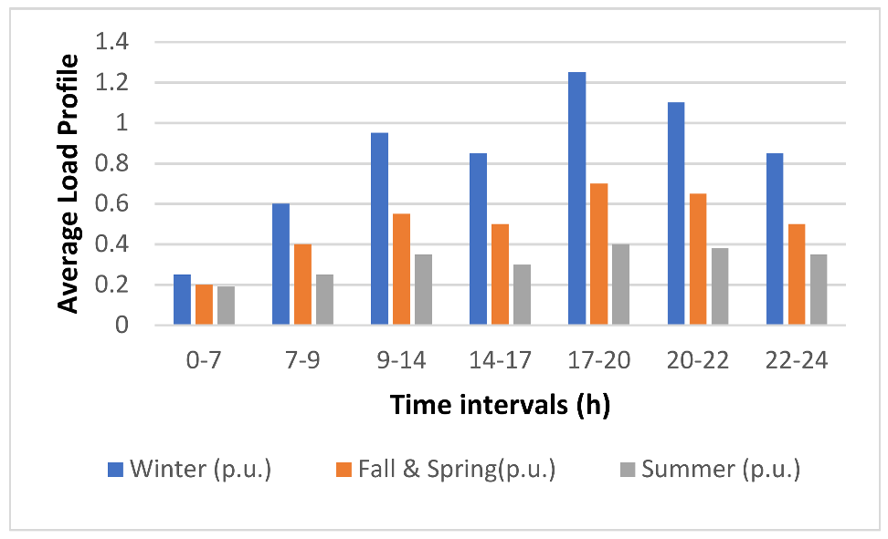
Most of the loads in a power network vary with time. In addition to the daily variation of loads, the load profile also depends on the seasons and weather conditions during a year. Thus, the daily load profile should be considered variable for each season of a year. As the weather condition does not change that much in a season, the load demand and consequently, the daily load profile, can also be considered identical during a season. Figure 1 shows the average daily load variation for different seasons and different time intervals.

For simplicity, the daily load profile can be divided into intervals over which the load is assumed to be constant. This constant value is calculated from the load curve by averaging using the Trapezoidal method. The data for the load curve are extracted from [10]. It should be noted that these amounts are the average of the load for weekdays and weekends.

As mentioned earlier, the period of the study in this paper is assumed to be the same as the lifetime of the DGs. The lifetime of the resources is considered to be 10 years. The load demand is growing every year due to increasing population and usage of electrical devices. Therefore, load growth should be considered in the period of the study, which is assumed to be 2% every year [6]. For considering 10 years of planning, the numbers in the above table would extend to 70 time intervals for the 10 years, where the number in each time interval is multiplied by 1.02 for each year.

2.2. Objective Function

For the aim of this project which is minimizing the total cost, the objective function should consist of the cost of investment, operation and maintenance (O&M), and also the energy losses in the power network. Losses have thermal effects on the lines of a network and are measured in Watts. However, the costs of investment and O&M of DGs are measured in dollars and are based on monetary units. Therefore, it is required to change the loss model into monetary units.

The cost function is generally as follows:

$$Objective function= {\displaystyle \sum }_j{I}_j\ast capacity of the j\mathrm{th} DG+ {\displaystyle \sum }_i{\displaystyle \sum }_j{\left(O\&M\right)}_j\ast {\left(power generated by DG\right)}_{i,j}\ast T_i+{\lambda }_{grid}\ast x_{grid}\ast T+F\left(losses\right)$$

(1)

where, $I_j$ is the investment cost of the jth DG in $/kW, ${\left(O\&M\right)}_j$ is the operation and maintenance cost of the jth DG in $/kW, ${\left(power generated by DG\right)}_{i,j}$ is the power produced by the jth DG at the ith time interval. $T_i$ is the duration of the ith time interval for each year. ${\lambda }_{grid}$is the price of buying electricity from the external grid. $x_{grid}$is the power supplied by the external grid. In planning, the max load should be considered in order to supply the demand. In this paper, at every time interval, the exact amount of load will be considered and for supplying extra power required, electricity will be bought from the external grid. T is the total duration of the period of planning which in this case is 8760 h multiplied by 10, the useful life time of resources, and $F\left(losses\right)$ is the losses cost function. In the above formula, DGs can be diesel generators or wind turbines.

If there is no DG in the power system, cost of losses would be equal to the cost of buying electricity from external grid. This is the result of the assumption that all of the losses in the network are supplied by the grid. However, by installing DGs in the network, the losses may be supplied by them, and thus, the cost of grid and losses would be different due to the fact that the price of buying electricity from them is different from the external grid.

It should be noted that in some cases, the output power of the DGs may be greater than the total demand at that moment. In such cases, the external grid absorbs the extra power. In other words, in some time intervals, power may be sold to the grid. If this condition occurs, $x_{grid}$ will be negative and will minimize the cost function.

The constraint is that the total power generated by the DGs should be as close as possible to the total demand at every moment. In the case of diesel generators, the output power can be determined, but if wind turbines are used in the system, the output power would be fixed according to the wind speed. Thus, this constraint is obtained just by installing diesel generators in the system. These criteria lead to less power absorption from the external grid. Thus, in the case of outage, dependence on the external grid would be minimum. To formulate this limitation, the difference between the total demand and total power generated is set to 5% of the total load.

2.3. Loss Modeling

Network losses in a micro grid depend on the grid configuration, DGs’ location, and grid node connection. Due to the investment and operational costs, it becomes important to know what percentage of the network power losses is supplied by the DGs and grid. One simple method to use is the postage stamp method to consider the power loss shares in a micro grid which is explained in [11]. Based on this method, the formula of the losses of the system can be written as:

$$los{s}_{DG}=Total loss\ast \frac{P_{DG}}{\sum P_{DG}+ P_{grid}}$$

(2)

$$los{s}_{grid}=Total loss\ast \frac{P_{grid}}{\sum P_{DG}+ P_{grid}}$$

(3)

where $P_{DG}$ is the active power generated by the DGs, irrespective of whether they are wind turbines or diesel generators, and $P_{grid}$ is the active power generated by the external grid.

Based on Equations (2) and (3), the cost of losses can be computed as follows:

$$F\left(losses\right)= (los{s}_{DG}\ast {\lambda }_{DG}+ los{s}_{grid}\ast {\lambda }_{grid})\ast T$$

(4)

where ${\lambda }_{grid}$ is the price of buying electricity from the external grid and ${\lambda }_{DG}$ is the price of buying electricity from each DG. T is the total duration of the planning period, and ${\lambda }_{DG}$ is calculated from Equations (5)–(7):

$$i_{eq}=i+f+i\ast f$$

(5)

$$A= \frac{{\left(1+i_{eq}\right)}^n-1}{i_{eq}\ast {\left(1+i_{eq}\right)}^n}$$

(6)

$${\lambda }_{DG}= \frac{I}{A\ast 8760}+ \frac{O\&M}{8760}$$

(7)

where i is the rate of return, f is the inflation rate and n is the average lifetime of DGs. $i_{eq}$ shows the equal rate of return of a system which has an inflation rate [13]. It should be noted that the O&M cost is in $/MW/year. Thus, this cost should be divided by 8760 in order to be in $/MWh. Equations (6) and (7) convert the O&M cost into the price of buying electricity from each DG [13].

In the case of the inflation rate, the equal rate of return should be defined which is obtained from Equation (5). In Equation (6), the investment cost is converted to the annual payment in each year, and then, the total annual payment is divided by 8760, and therefore, ${\lambda }_{DG}$ is obtained in $/kWh.

It should be noted that the DG could be different with various lifetime averages and investment costs. Thus, ${\lambda }_{DG}$ changes according to the type of DG, i.e., wind turbine or diesel generator.

2.4. Constraints

Every optimization function has some constraints which restrict the feasible answers. In a power network, there are two major constraints:

• Limits of bus voltages: The voltage of all of the busses in a power network should remain within a standard range. This range is defined by IEEE or IEC standards and is assumed to be ±5%. In other words, all bus voltages must be between 0.95 and 1.05 per unit, i.e.,

  $${0.95}^{\mathrm{p}.\mathrm{u}.}< V_i< {1.05}^{\mathrm{p}.\mathrm{u}.}\hspace{1em}i\in \left\{all of the busses\right\}$$

  (8)
• Limits of line loadings: all of the lines of a power network have some intrinsic parameters. One of them is the capacity of the current flowing in the lines. This limitation is due to the thermal effects of flowing currents in the lines. For optimization, this line limit is assumed to be 105%.

2.5. PSO Algorithm

There are many algorithms for optimizing customized objective functions which are based on natural phenomena. One of the most common and useful methods is the PSO algorithm. This algorithm models the objective function as the particle swarm movement. Based on PSO, in order to optimize the objective function, some particles should be considered. These particles are initialized randomly, and after computing the objective function for each particle, the best particle which minimizes the objective function is selected. Then, the particle is updated and this procedure is repeated until the optimal answer is reached. Now, the array of the particle should be determined.

In this paper, the goal is to find the best location of the DGs in the network such that the cost function is minimized, and all of the constraints are satisfied. The DGs in the first scope of the work could be wind turbine or diesel generators. In other words, in the first step, all of the DGs that are placed in the buses of the network are of one of the two types that are mentioned before. It is considered here that the busses of the network are the same in the scope of wind speed and there is no preference in the busses of the system for allocating DGs. For using the PSO algorithm in the optimization problem, two cases should be defined: using just diesel generators and using just wind turbine.

The difference between these two cases is in the output power of the DGs. For diesel generators, as mentioned before, the output power could be determined. Alternatively, for wind turbines, the output power is fixed and is based only on the wind speed. Thus, each case should be investigated separately.

• Case 1, Diesel generators: the other variable that should be determined, besides determining the location of DGs, in the procedure of the optimization is the output power of the DGs in each time interval for each season of each year. Thus, the desired particle is as follows:

  $$\left\{\begin{array}{c}first place of the DG | output power of the DG for\\ \left(3\ast T\ast 10\right) time intervals\left|second place of the DG \right|\dots \end{array}\right\}$$

  (9)
  The first place of the particle array is the number of the bus at which the first DG must be placed. In the next bits of the array, the power generated by that DG at every time interval will be found. T is the number of time intervals in each day; 3 is the number of seasons in the year (considering that fall and spring seasons modellings are the same); and 10 is the number of the years in the period of the study which is the average life time of resources.
  In other words, the array which shows the power generated by each DG looks like Equation (10):

  $$\left\{{\left\{Winter \left| Fall/Spring\right|Summer\right\}}_1, \dots , {\left\{Winter \left| Fall/Spring\right|Summer\right\}}_{10}\right\}$$

  (10)
  In the above equation, the indices of the arrays show the number of the year in the period of study.
• Case 2, wind turbines: In this case, the only variable that should be determined is the capacity of the wind turbine besides the location where the wind turbine is connected to the network. The amount of power produced in each time interval and each year would be obtained by considering the wind speed at every moment. Thus, in the first step, the wind speed should be noticed and investigated. Figure 2 shows the output power of a typical wind speed capacity of 500 kW [10].

Figure 2. Daily patterns for hourly average power generation for a 500-kW wind turbine [10].

Figure 2. Daily patterns for hourly average power generation for a 500-kW wind turbine [10].

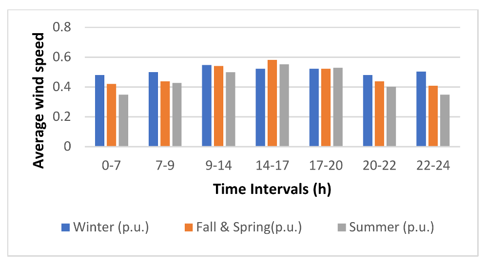
As the output power of the wind turbine has a direct relationship with the wind speed, the numbers of the vertical axis of the curve in Figure 2 could be scaled per unit and generalized to the capacity needed in a custom power network. Also, the wind speed could be determined for every time interval in each season of a year. Figure 3 shows the scaled number for the time intervals, the same as that considered for the load demand. It should be noted that the wind profile for a specific region will be constant for every year and will not be changed during the period of study.

$$\left\{bus numbe{r}_1 \left| capacit{y}_1 \right| bus numbe{r}_2 \left| capacit{y}_2\right|\dots \right\}$$

(11)

The capacity obtained here will be multiplied by the numbers of Figure 3. The results are the output power of each wind turbine during the period of study.

Based on the number of DGs needed in the network, this particle will be extended and repeated in the same manner. By considering this particle and after some iterations, the final result will be obtained. This result will represent the locations and sizes of all the DGs.

2.6. Different Scenarios

In a power system, there is a limitation in using wind turbines, due to uncertainties and the harmonics that insert to the network and we should implement some diesel generators beside wind turbines. Thus, different scenarios will be created based on the number of diesel generators. The following scenarios show different cases to which the PSO algorithm is applicable to all. In all of the scenarios, it is assumed that 5 DGs could be installed in the busses of the network. Therefore, the summation of the number of diesel generators with wind turbines should be 5, the same as previous sections. Thus, different scenarios would be as follows:

• Scenario 1: 5 diesel generators, 0 wind turbines. This case is identical to case 1 of part E. Therefore, the desired particle is the same as that mentioned there.
• Scenario 2: 4 diesel generators, 1 wind turbine. In this case, the capacity of the only wind turbine beside the power produce by each DG during the period of study should be defined. The desired particle is as follows:

  $$\left\{B_1 \left|output power for\left(3\ast T\ast 10\right) time intervals |\dots \right|B_5| C_5\right\}$$

  (12)

  where $B_i$’s are the bus numbers in which ith DG will be installed. $C_5$ is a number between 0 and 1 which is per unit and by considering the specification of the network, determines the capacity of the wind turbine.
• Scenario 3: 3 diesel generators, 2 wind turbines. For this case, the desired particle is as follows:

  $$\left\{B_1 \left|output power for\left(3\ast T\ast 10\right) time intervals \left|\dots |B_3 \right|\dots \right|B_4\left| C_4\right| B_5| C_5\right\}$$

  (13)
• Scenario 4: 2 diesel generators, 3 wind turbines. For this case, the desired particle is as follows:

  $$\left\{B_1 \left| output power for\left(3\ast T\ast 10\right) time intervals\left| B_2\right|\dots \right| B_3\left| C_3\right| \dots | B_5| C_5\right\}$$

  (14)
• Scenario 5: 1 diesel generator, 4 wind turbines. For this case, the desired particle is as follows:

  $$\left\{B_1 \left| output power for\left(3\ast T\ast 10\right) time intervals\left| B_2\right| C_2\right| \dots \left|B_5\right| C_5\right\}$$

  (15)
• Scenario 6: 0 diesel generators, 5 wind turbines. This case is identical to case 2 of part E. Therefore, the desired particle is the same as that mentioned there.

In the next section, the cost function for each of these scenarios will be calculated and the best case of using both diesel generators and wind turbines will be defined.

It should be noted that the PSO algorithm operates the same for all of these 6 scenarios. The only difference is the particle definitions which are defined for all of the cases.

3. Particle Swarm Optimization (PSO) Algorithm

PSO is a heuristic optimization algorithm developed in 1995, inspired by social behavior and the movement of bird or fish migration.

PSO shares many similarities with other heuristic methods such as GAs. The system is initialized with a random solution and is optimized by updating the particle position. However, unlike GA, PSO has no feature of crossover and mutation. In PSO, the potential solutions, called particles, can be changed in the problem space by following the current optimum particle.

PSO is very easy to implement compared to GA and there are few parameters to adjust and has been successfully applied in many areas such as power networks.

PSO uses a set of particles, representing potential solutions. The particles move around in a search space with a position $x_i^t$ and a velocity $v_i^t$, where i represents the index term of the particle and t is the time. For each iteration, the particle compares its current position with the best position and adjusts its velocity towards the goal [14]. Then, the velocity and particle position can be updated by using the two following equations:

$$v_i^{t+1}=w v_i^t+c_1\ast rand\ast \left(p_i^t- x_i^t\right)+c_2\ast rand\ast \left(p_g^t- x_i^t\right)$$

(16)

$$x_i^{t+1}= x_i^t+ v_i^{t+1}$$

(17)

where c₁ and c₂ are positive constants defined as acceleration coefficients and set to be 1.7. w is the inertia weight for accelerating the convergence speed of PSO algorithm and is set to 0.6. rand is a random function in the range of [0, 1]. $p_i^t$ is the best previous position of $x_i^t$ and $p_g^t$ is the position of the best particle among the entire population.

4. Simulation

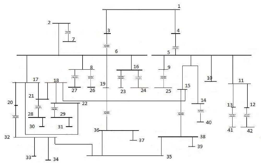
To evaluate the performance of the proposed method, an IEEE std 39 network is selected as the test system. This sample network is a distribution system with 42 buses. Busses 1 to 4 have a voltage level of 69 kV, busses 5 to 22 have a voltage level of 13.8 kV, busses 23 to 26 have a voltage level of 2.4 kV, and the other busses have a voltage level of 480 V. The external grid is connected to one of the 69 kV busses, and all of the loads are connected to the 480 V and 2.4 kV busses. It is assumed that the DGs are to be placed at the 13.8 kV and 2.4 kV busses. The general topology of the network is shown in Figure 4. The specifications of the lines can be found in [15].

It is assumed that 5 DGs are to be placed in the network. In other words, 5 busses should be selected in order to install the DGs. This number comes from the assumption that 12% of the total number of busses is suitable for allocating DGs. A number higher than this yields an unstable and uncontrollable system [16]. By this assumption and considering 42 busses in the standard system, the best number of busses for allocating DGs is 5. In the particle array, the amount of power produced by each DG is considered to be between 0 and 1. Then, this number is multiplied by the capacity of the DGs. The capacity of the DGs depends on the voltage of the bus to which the DG is connected. In other words, if the DG is connected to one of the 13.8 kV busses, it is assumed that it could produce 5.75 times more power than the one that is going to be connected to the 2.4 kV busses. The number 5.75 is computed by the division of 13.8 by 2.4. This number shows the importance of busses with voltage of 13.8 kV. By this assumption, the busses with higher voltage could produce more power than other busses.

For obtaining the capacity of the wind turbines in the study case, the maximum demand of the system in the duration of the period of the study should be determined. Equation (16) shows the maximum demand of the system based on the total load and rate of growth of the loads in the system.

$$P=Tl\ast 1.25\ast {(1+LG)}^{10}$$

(18)

In the above equation, Tl shows the summation of the nominal loads in the network. Maximum load occurs in the winter and is 1.25 times more than the nominal load. LG shows the rate of growth of the loads which is considered to be 2%.

With the above consideration, the capacity of the wind turbines at the 13.8 kV busses and at the 2.4 kV busses is given by the following equations, respectively.

$${C_{wind}}_i= C_i\ast 5.75\ast \frac{P}{{{\displaystyle \sum }}_{j=1}^{5}5.75\ast a_j + {{\displaystyle \sum }}_{j=1}^5{b}_j}$$

(19)

$${C_{wind}}_i= C_i\ast \frac{P}{{{\displaystyle \sum }}_{j=1}^{5}5.75\ast a_j + {{\displaystyle \sum }}_{j=1}^5{b}_j}$$

(20)

In these equations, $C_i$ is the capacity of the ith wind turbine, which appears in the array of the particle and is between 0 and 1. $P$is the maximum demand which is obtained from Equation (16). $a_j$ is the location of the jth DG, which is a binary number and shows whether the DG is placed at 13.8 kV busses. $b_j$ is the same as $a_j$ except for the 2.4 kV busses.

For defining the power produced by diesel generators in the different scenarios mentioned before, the power produced by wind turbines should be subtracted from the total load at every time interval. The remaining demand should be supplied by diesel generators. The output power of wind turbines is defined by the following equation:

$$P_{win{d}_{i,j}}=C_{win{d}_i}\ast C{o}_j$$

(21)

$P_{win{d}_{i,j}}$ is the power of ith wind turbine in jth time interval. $C{o}_j$ represents the per unit output power of wind turbines based on wind speed for the jth time interval, which is shown in Figure 3. By considering the above equation, the output power of diesel generators at the 13.8 kV busses and at the 2.4 kV busses is given by the following equations, respectively.

$${P_{DG}}_{ij}= P_{ij}\ast 5.75\ast \frac{T{L}_j- {{\displaystyle \sum }}_{i=1}^{n_{wind}}{P}_{win{d}_{i,j}}}{{{\displaystyle \sum }}_{i=1}^{5-n_{wind}}5.75\ast a_i + {{\displaystyle \sum }}_{i=1}^{5-n_{wind}}{b}_i}$$

(22)

$${P_{DG}}_{ij}= P_{ij}\ast \frac{T{L}_j- {{\displaystyle \sum }}_{i=1}^{n_{wind}}{P}_{win{d}_{i,j}}}{{{\displaystyle \sum }}_{i=1}^{5}5.75\ast a_i + {{\displaystyle \sum }}_{i=1}^5{b}_i}$$

(23)

Using Equations (20) and (21), the output power at each time interval is obtained and the cost function can be computed. The number of iterations is supposed to be 100 and the number of particles is 20.

The coefficients of the load curve is shown in Figure 1. According to this figure, considering 7 time intervals seems reasonable. The base amounts of the loads are given in

Table 1. The active and reactive power demand.

Load	Active Power (MW)	Reactive Power (MW)	Load	Active Power (MW)	Reactive Power (MW)	Load	Active Power (MW)	Reactive Power (MW)
1	1.237	0.701	11	0.31	0.2	21	1.27	0.72
2	0.52	0.32	12	0.32	0.19	22	1.38	0.78
3	0.3	0.18	13	0.08	0.06	23	1.8	1.02
4	0.25	0.15	14	0.08	0.06	24	0.85	0.48
5	0.062	0.042	15	0.26	0.16	25	6.36	0
6	0.17	0.11	16	0.17	0.11	26	0.96	0.52
7	1.77	1	17	0.4	0.24	27	0.35	0.2
8	0.46	0.27	18	0.32	0.2	28	0.96	0.52
9	0.2	0.12	19	0.35	0.23	29	0.15	0.049
10	0.42	0.28	20	0.52	0.32	30	0.12	0.08

. These numbers are multiplied by the numbers from Figure 1, and the daily load curve is estimated.

For diesel generators, the investment cost is 4000 $/kW. The O&M cost is considered to be 300 $/kW per year [12]. For wind turbines, the investment cost is 5500 $/kW and the O&M cost is considered to be 200 $/kW per year [12]. By considering the lifetime average of these DGs to be 10 years, the inflation rate of 15% and rate of return of 20%, ${\lambda }_{DG}$’s can be obtained from Equations (5)–(7). The result is 0.18 $/kWh for diesel generators and 0.24 $/kWh for wind turbines. ${\lambda }_{grid}$ is assumed to be 0.25 $/kWh.

5. Results

By applying the proposed method to the IEEE radial standard network, the amounts of the total cost function for different scenarios are given in the

Table 2. Cost results in detail.

Scenarios	Costs ($)
1	$244,526,333 \$$
2	$222,626,450 \$$
3	$210,622,441 \$$
4	$143,133,094 \$$
5	$133,589,005 \$$
6	$144,435,042 \$$

.

By comparing the numbers of Table 2, it is obvious that scenario 5 has the least cost function among others. In this scenario, the best locations of DGs are given in the

Table 3. Location of distributed generations (DGs) in Scenario 5.

Location of DGs	Bus Number
Diesel generator 1	17
Wind turbine 1	4
Wind turbine 2	22
Wind turbine 3	5
Wind turbine 4	19

.

By considering Table 2, it is obvious that by increasing the number of wind turbines in the system, the total cost of installing them is reduced. This reduction is due to the O&M cost which is less than the O&M cost of diesel generators. It should be noted that the investment cost of wind turbines is more than the investment cost of diesel generators. As the period of study is 10 years, this cost is distributed over long time and so it does not affect the total cost.

By the above explanation, it is expected that minimum cost would be achieved in scenario 6. But in the last scenario, all of the DGs in the system are wind turbines. In this case, there is no flexibility and control in producing power and only the capacity of the DGs could be determined. The total power for supplying the total demand is dependent on the wind speed. In some cases in which the wind speed is not sufficient, the remaining demand would be supplied by the external grid which increases the cost function, due to the higher price of buying electricity from the grid and increases in the losses in the network.

In scenario 5, the number of wind turbines is more than that for the other 4 scenarios and there is 1 diesel generator for controlling and supplying the remaining power. Thus, the results of Table 2 are reasonable.

Finally, the amount of production by each DG is obtained from the optimization. These amounts are as shown in

Table 4. Optimum power generation profile and the location of the DGs.

The amount of production for each time interval during the year which appeared in the particle array (p.u.)	Location (Bus Number)
	17	4	22	5	19
	0.39	0.29	0.82	0.39	0.15
	0.45	0.78	0.43	0.76	0.8
	0.29	0.16	0.52	0.07	0.27
	0.47	0.85	0.3	0.44	0.41
	0.84	0.79	0.89	0.23	0.51
	0.29	0.56	0.12	0.89	0.64
	0.52	0.0011	0.95	0.38	0.02
	0.11	0.29	0.5	0.7	0.16
	0.8	0.83	0.64	0.3	0.87
	0.44	0.77	0.37	0.35	0.71
	0.74	0.91	0.92	0.79	0.74
	0.3	0.19	0.43	0.7	0.67
	0.9	0.61	0.73	0.6	0.28
	0.44	0.73	0.27	0.74	0.15
	0.16	0.61	0.72	0.6	0.09
	0.31	0.2	0.19	0.93	0.39
	0.92	0.24	0.59	0.18	0.72
	0.998	0.07	0.3	0.72	0.53
	0.739	0.14	0.7	0.2	0.88
	0.65	0.22	0.96	0.98	0.35
	0.049	0.42	0.98	0.08	0.16

.

6. Conclusions

In this paper, a DG placement is proposed which simultaneously optimizes system energy losses as well as the investment and O&M costs. Type of DGs could be wind turbine or diesel generators. For every DG, a power profile can be obtained which represents the power produced by each DG at each time interval of 10 years. These numbers are based on minimizing a cost function which consists of the cost of investment and O&M of the DGs and also the cost of buying electricity from the external grid. Losses are also modelled as a cost function and are included in the objective function.

Different scenarios are investigated in which the number of diesel generators and wind turbines changes from 0 to 5. The results show that the proposed method yields more economical planning for installing DGs in a micro grid and determines the best number of wind turbines versus diesel generators with their best locations.