Article

Impedance Modelling and Parametric Sensitivity of a VSC-HVDC System: New Insights on Resonances and Interactions

by
Adedotun J. Agbemuko
1,*,
José Luis Domínguez-García
1,
Eduardo Prieto-Araujo
2 and
Oriol Gomis-Bellmunt
2
1
Electrical Power Systems Area, Catalonia Institute for Energy Research, 08930 Barcelona, Spain
2
CITCEA-UPC, Department of Electrical Engineering, Polytechnic University of Catalonia (UPC), 08028 Barcelona, Spain
*
Author to whom correspondence should be addressed.
Energies 2018, 11(4), 845; https://doi.org/10.3390/en11040845
Submission received: 13 January 2018 / Revised: 29 March 2018 / Accepted: 2 April 2018 / Published: 4 April 2018
(This article belongs to the Section F: Electrical Engineering)

Abstract

:
Pervasiveness of power converters in the electric power system is expected in the future. Such large penetration will change the current power system dynamics leading to uncertain, unexpected, and potentially critical responses. This paper investigates the stability and resonance of a VSC-HVDC (Voltage Source Converter High Voltage Direct Current) link within an AC grid, whilst providing insights into resonances having a role on the grid. This is studied through the impedance-based modelling of the entire system (AC and DC grids), including controls of converters. Additionally, the impact of the different parameters of the hybrid AC-DC power system such as control systems and grid components on the system dynamics and stability is investigated. From this study, the impact of the system components and the controls of the converter on overall resonance response and stability is shown, including potential undesired sub-synchronous and harmonic resonances due to AC-DC system interactions. The analytical impedance-based models developed and obtained is validated through time-domain simulations, the physical model of the whole system is built in Simscape Power Systems and control systems in MATLAB/Simulink® (R2017b). This has demonstrated the validity of the model to deal with and detect such dynamics.

1. Introduction

The rapid increase and integration of renewable energy sources (RES) and new generation technologies such as electric vehicles, fuel cells, and battery storage has led to a huge demand for power electronic converters in today’s power systems. Such penetration level is expected to further increase into the future [1]. The voltage source converter (VSC) is the state-of-art of power converters for the transmission system and, indeed, a majority of these resources are expected to be integrated through power electronic converters based on VSC technology [2], and further use driven by the undesirable characteristics of line commutated converter (LCC) technology [3]. The VSC-HVDC (Voltage source converter High voltage direct current) is fast becoming the technology of choice for high power transmission, grid expansion, and strengthening, with the potentials to become the backbone of future transmission system [4]. Evidently, the power system is progressing towards a hybrid nature, combining the AC and DC grids, modifying its dynamic response and behaviour. Therefore, with the expected ubiquity of converter interfaces, particularly VSC technologies at the transmission level, harmonic stability and resonance issues must be revisited.
The challenges of extensive use of power converters cannot be overemphasized as detailed in the surveys, [5,6]. A growing issue in the industrial community is the influence of often complex control strategies of converters and grid parameters (AC/DC) on the resonance and oscillatory behaviour of the entire system. A significant number of ground-breaking works have studied the harmonic resonance and interactions due to power electronic interfaces in distributed generation systems interfaced with the AC grid [7,8,9,10,11,12,13]. However, many of research efforts have focused mainly on the AC grid, effectively neglecting the DC side dynamics; nevertheless, this is justifiable at a microgrid level where there is only one source. However, at higher voltage levels, DC voltage control is a prerequisite. At such a level, the DC voltage is a carrier of oscillations of varying bandwidths that could potentially transfer to the AC grid through the control. These are network and control induced oscillations and there is little literature on identifying which network components and control parameters play a role.
A method that has been gaining considerable attention and successfully applied in literature is the impedance-based modelling methodology as a tool for resonance and interaction analysis [13,14,15,16,17,18,19]. The research community have attempted to apply impedance-based models considering the influence of power electronic converters to understand sources of resonances at the device level [15,20,21,22,23]. Similarly to most of the works, the network is often assumed to be ideal; particularly, the DC side. Furthermore, with countless variables across two distinct grids, linked by a tightly controlled device, it is not clear exactly what influences the observed oscillatory responses despite the device itself been clearly stable.
More recently, the impedance-based method has been applied to understand the sources of harmonic instability and resonance phenomena in wind power plants integrated by VSC-HVDC converters with outstanding results [24,25,26,27,28]. However, wind power plant networks often have unique topologies, and controls, and observed oscillatory behaviours that are difficult to generalize. In addition, in a significant number of works, the DC side is often ignored. In cases where the DC voltage control loops were included, the DC voltage dynamics is often based only on the terminal capacitance and neglecting the impact of network and impedances of other connected devices. Thus, very few works have explicitly considered the DC side of the VSC-HVDC system. In [29,30], both AC and DC grids were modelled by separating the rectifier and inverter, and impedance models of each derived. However, authors mainly demonstrated the impact of power transfer level amongst other factors on the DC resonances and instabilities. In other efforts, the DC grid was modelled based on a single-input single-output (SISO) system, [31] and multiple-input multiple-output (MIMO) system [32]. However, resonance analysis was restricted to the DC grid and the impact of DC resonances on AC systems was not studied. More recently, the impedance model for resonance analysis has been applied to a real back-to-back VSC-HVDC system to analyse resonances between the AC grid and converter [33]. In view of these, there is a lack of literature on a system level impact of the entire system; DC, AC grids, and control on dynamic responses observed in a VSC-HVDC linked AC grid.
This paper explicitly considers the AC grid and entire DC grid dynamics modelled by the nodal impedance matrix, which considers network topology, and impedances as seen from the view of the grid connected converter. This offers flexibility in terms of connection or disconnection of any component, or simplifications thereof, without remodelling the entire system. Furthermore, this paper provides a clear understanding to the interactions between VSC based HVDC system linked with an AC grid, through analytical and simple model development of both grids. This paper also attempts to fill the gaps on AC/DC interaction by employing the impedance-based modelling to a VSC-HVDC link integrated with an AC grid. In this case, this is carried out by considering models of both sides, trying to cope with both at the same time without special focus on AC or DC, as usually is done. Additionally, the model in frequency domain has been derived allowing to include explicitly the control system in analysis. Additionally, the equivalent feedback impedances on both sides of the converter are derived in a tractable manner suitable for studies. Subsequently, parametric sensitivities on frequency response of derived impedances is carried out to identify parameters that impact the shape of these impedances. This is an attempt in understanding how parametric changes may contribute to detrimental oscillations in the AC grid transferred from the DC grid. Furthermore, the effect of DC grid and controller parameters are emphasized and stability analysis carried out. Ultimately with this method, computationally expensive and time-consuming analysis would not be necessary if similar conclusions can be drawn from the frequency domain analysis.
The paper is organized as follows: Section 2 presents the system under study, Section 3 introduces the impedance-modelling procedures of the system under study from the physical system, to each control in the cascaded structure and subsequently the aggregation of all derivations. Parametric sensitivities to obtain insight on how parametric changes impact system responses during disturbances are presented in Section 4. Finally, conclusions are drawn in Section 5.

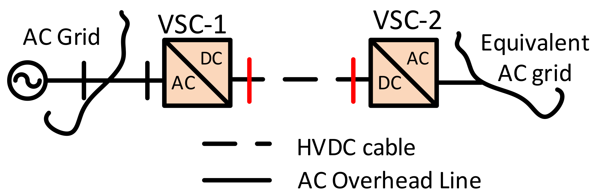
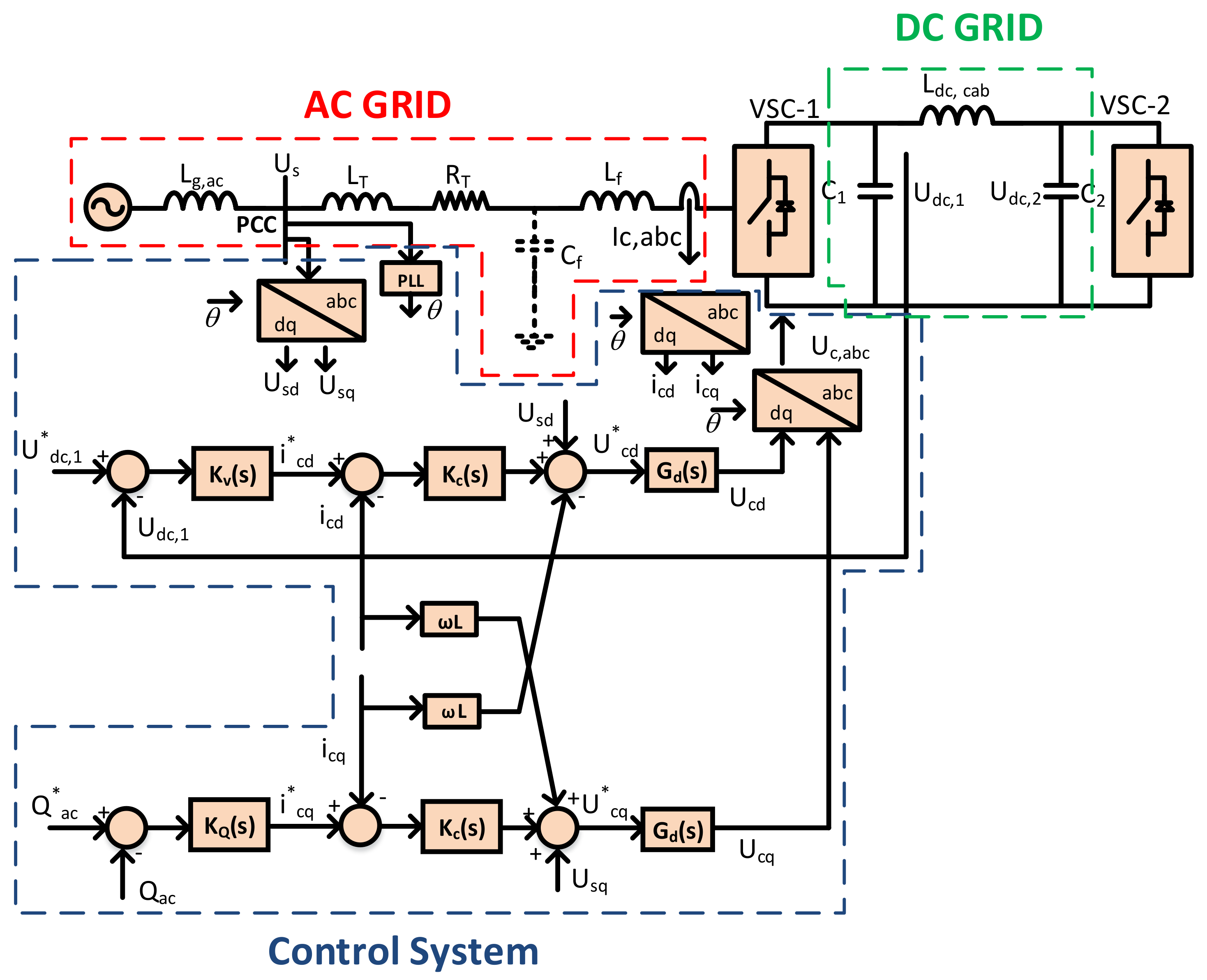
2. System Description and Control System

The system under study is a VSC-HVDC monopole link depicted in Figure 1. The AC side consists of the converter filter inductor, filter capacitor, transformer, and the Thévenin equivalent impedance of the connected AC grid, whereas the DC side is modelled by equivalent capacitances at each converter terminal and DC cable impedance. Figure 2 depicts the impedance circuit model and associated control system. The point of common connection (PCC) is taken as the high voltage side of the converter transformer. VSC-1 controls the DC voltage while VSC-2 controls the active power.
The control systems is implemented in the synchronous rotating d q -reference frame (SRF) using Park’s transformation [34]. Therefore, allowing both active and reactive power components to be controlled independently. Thus, each VSC is equipped with a decoupled inner current controller whose reference is provided by the outer controllers such as reactive power and DC voltage. In order to properly understand the impact of different controller bandwidth, it is assumed that AC voltages are perfectly sinusoidal. This is equivalent to assuming a strong grid connection. All controllers including the inner current controller employ proportional-integral (PI) compensators. Reactive power is assumed to be zero and the effect of q-axis on which the reactive power is implemented is insignificant.

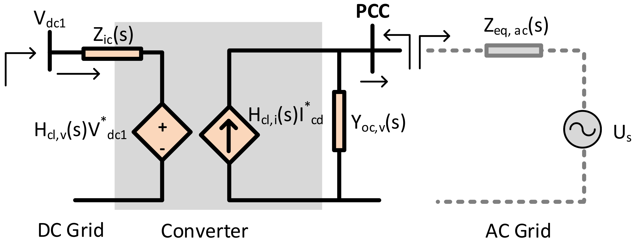
3. Impedance Modelling of the System

At a physical level, resonances and oscillatory behaviour in a system are mainly dictated by the primitive impedances and topology of the network. In the presence of a tightly controlled device such as a converter, its control interacts with the physical system made of primitive impedances in a complicated manner. That is, the converter through its control changes the primitive impedance of the system at the point of connection. Hence, the converter and the dynamics of its control can be modelled by a feedback impedance at the point of connection on both sides (AC and DC). In literature, this impedance is generally referred to as output or input impedance depending on the power direction. Thus, AC output impedance (or admittance) implies the converter is in inversion mode and the corresponding impedance on the DC side is an input impedance. Note, impedance and admittance without loss of generality may be used interchangeably as employed in this work. This makes no difference and is only used to maintain consistency of mathematical equations where necessary.
Therefore, the final goal in this section is to obtain the feedback impedance of the converter and its control, starting with the physical system, next, the lowest level control, up to the outermost loop. Each control loop imposes a corresponding impedance at the input or output of the converter. As such, the impedance of an outer loop would evidently include that of the inner loop, whilst the inner loop would include the impedance of the physical system as depicted in Figure 3. This is evident in the following sections. Subsequently, the control loops are tuned to obtain a reference case for comparison in a later section on sensitivity.

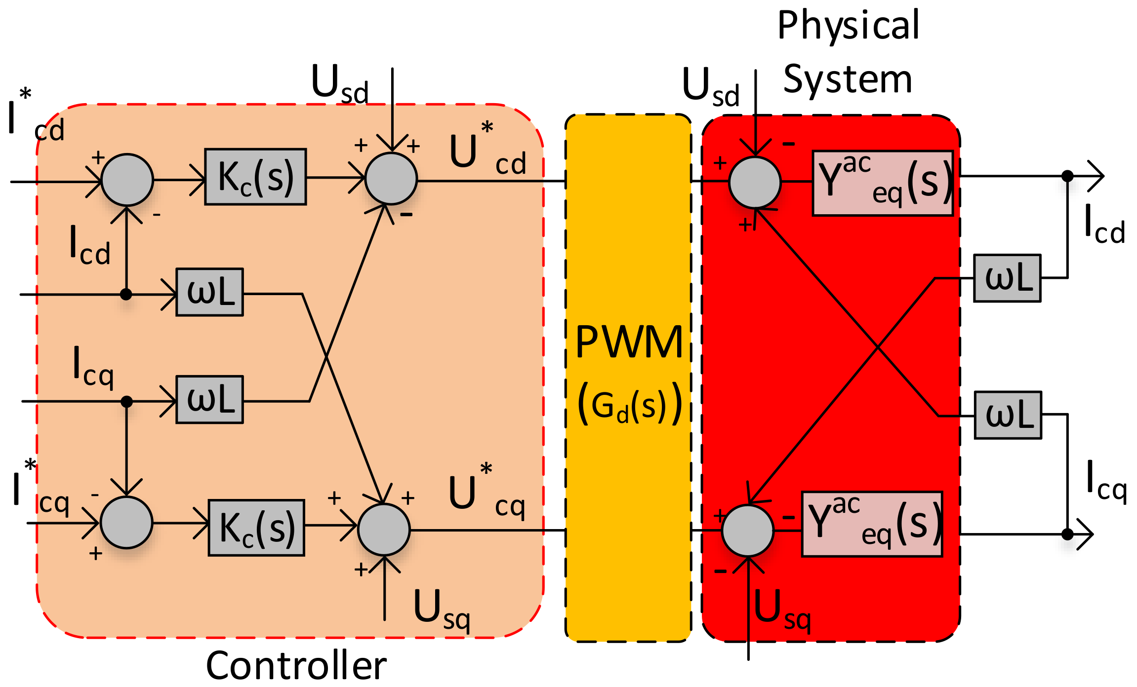
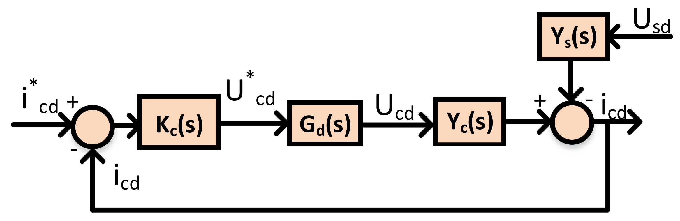
3.1. Analytical Modelling of the Inner Current Controller

The AC grid is modelled based on balanced three-phase controllable voltage sources, thus allowing us to model one phase. From Figure 2, the AC current dynamics in the dq domain can be modelled by the open-loop (circuit) expression given by
i c , d q ( s ) = Y c ( s ) U c , d q ( s ) - Y s ( s ) U s , d q ( s ) ,
where i c , d q is the converter AC side current in the dq frame; Y c ( s ) and Y s ( s ) define the primitive admittances as seen from the converter and grid respectively, given in Equations (2) and (3)
Y c ( s ) = Z t ( s ) + Z c f ( s ) Z t ( s ) Z c f ( s ) + Z t ( s ) Z f ( s ) + Z c f ( s ) Z f ( s ) ,
Y s ( s ) = Z c f ( s ) Z t ( s ) Z c f ( s ) + Z t ( s ) Z f ( s ) + Z c f ( s ) Z f ( s ) ,
where Z t ( s ) = R t + s L t , Z f ( s ) = s L f , Z c f ( s ) = 1 / s C f are the transformer, filter inductor, and filter capacitor impedances, respectively. Figure 4 depicts the analytical block diagram of the AC current loop on the d-axis with the primitive admittances from the AC side reflected on the control system. The closed-loop response equation can be derived as
i c , d q ( s ) = H c l , i ( s ) i c , d q * ( s ) - Y o c , i ( s ) U s , d q ( s ) ,
where H c l , i ( s ) (see Appendix B) is the closed-loop transfer function, given as
H c l , i ( s ) = H o l , i ( s ) 1 + H o l , i ( s ) ,
and H o l , i ( s ) is the open-loop gain, given as
H o l , i ( s ) = K c ( s ) G d ( s ) ( Z t ( s ) + Z c f ( s ) ) Z t ( s ) Z c f ( s ) + Z t ( s ) Z f ( s ) + Z c f ( s ) Z f ( s ) ,
and Y o c , i (see Appendix B) is the converter closed-loop output admittance on the AC side with only the inner current controller modelled, that is, the feedback impedance and can be derived as
Y o c , i ( s ) = Y s ( s ) 1 + H o l , i ( s ) ,
where K c ( s ) = k p i + k i i s is the inner-loop compensator, and G d ( s ) = 1 τ d s + 1 approximates the converter internal delay.
Figure 5 depicts the circuit representation of Equation (4) pre-connection with the AC grid. In order to establish a base case for the current controlled system, the current controller is tuned. Several methods are available in literature to find a controller K c ( s ) that meets specifications for the inner-loop. The internal model control (IMC), [35], is employed for tuning the AC inner-loop as it results in an ideal current controller and resonance-free feedback impedance (without considering grid impedance). Based on the IMC technique, the current controller is tuned to obtain a time constant τ of 2 . 5 ms. The impact of varying this time constant would be seen in later sections. Based on the IMC technique,
k p i = L τ ; k i i = R t τ ,
L = L t + L f is the total inductance of the transformer and filter, and R t is the resistance of transformer. Figure 6 depicts the frequency response plots of closed-loop output to reference transfer function, feedback impedance of the AC inner-loop, and time domain response of converter AC currents for step change in current. Particularly, the frequency response of feedback admittance show a flat response. Physically, this results in a resonance free operation as can be observed in the time domain response.

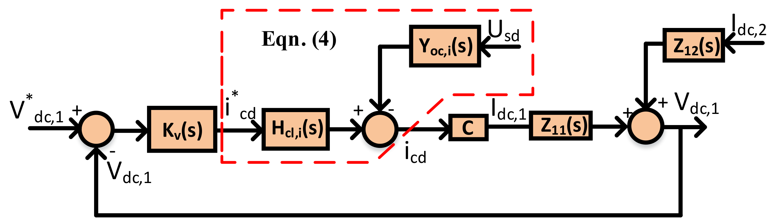
3.2. Analytical Modelling of the DC Voltage Controller

As previously mentioned, in a VSC-HVDC system, the DC voltage is often controlled in addition to the AC current control in a cascaded manner as depicted in Figure 2. Thus, the DC voltage control loop changes the output impedance of the converter on the AC side in addition to the AC inner-loop, and introduces an input impedance from the DC side. The DC voltage dynamics themselves depend on the network topology and structure; therefore, the entire DC grid and its structure is modelled by applying the nodal impedance matrix to obtain the DC voltage dynamics. The nodal equation of the DC grid can be derived as
V D C , 1 V D C , 2 = Z 11 ( s ) Z 12 ( s ) Z 21 ( s ) Z 22 ( s ) I D C , 1 I D C , 2 .
The detailed derivation of the nodal equation of the DC grid can be found in Appendix A. From Equation (9), the open-loop equation of the DC voltage at VSC-1 (plant to be controlled) can be re-written as, Equation (10),
V D C , 1 ( s ) = Z 11 ( s ) I D C , 1 ( s ) + Z 12 ( s ) I D C , 2 ( s ) ,
where Z 11 ( s ) is the Thévenin impedance of the DC grid as seen from VSC-1 and Z 12 ( s ) is the transfer impedance from the converter at VSC-2, derived as Equations (11) and (12). The DC cable is modelled by a Π equivalent with the end capacitances added to the DC terminal impedance as they are in parallel. Figure 7 depicts a proposed control system that directly reflects the dynamics of the DC grid on the DC voltage control loop, which provides reference to the AC inner-loop. The AC inner-loop is represented within the dashed line based on Equation (4):
Z 11 ( s ) = Z c 1 ( s ) ( Z D C , c a b ( s ) + Z c 2 ( s ) ) Z c 1 ( s ) + Z D C , c a b ( s ) + Z c 2 ( s ) ,
Z 12 ( s ) = Z c 1 ( s ) Z c 2 ( s ) Z c 1 ( s ) + Z D C , c a b ( s ) + Z c 2 ( s ) ,
where Z c 1 ( s ) = 1 / s C 1 , Z c 2 ( s ) = 1 / s C 2 , Z D C , c a b ( s ) = s L D C , c a b , are the impedances of the total capacitances C 1 and C 2 at each terminal (capacitance of cable included), and DC cable, respectively.
Employing block reduction techniques on Figure 7, the closed-loop response with the DC voltage controller can be derived as Equation (13):
V D C , 1 = H c l , v ( s ) V D C , 1 * - H A C / D C ( s ) U s , d + Z i c ( s ) I D C , 2 ,
H c l , v ( s ) = H o l , v ( s ) 1 + H o l , v ( s ) ; H o l , v ( s ) = C K v ( s ) H c l , i ( s ) Z 11 ( s ) ,
H A C / D C ( s ) = C Y o c , i ( s ) Z 11 ( s ) 1 + H o l , v ( s ) ,
Z i c ( s ) = Z 12 ( s ) 1 + H o l , v ( s ) ,
where H o l , v ( s ) , is the open-loop gain of the DC voltage control loop (see Appendix B), H A C / D C ( s ) is a disturbance gain from the AC-DC side, Z i c ( s ) is the DC input impedance, K v ( s ) is the DC voltage compensator based on PI, C is a constant obtained from the active power balance in Equation (17) [36], and P a c = P D C assuming a loss-less converter
3 2 ( U s d i c d + U s q i c q ) = V D C I D C .
From Equation (15), the output admittance on the AC side considering the impact of DC grid and DC voltage controller can be written as Equation (18)
Y o c , v ( s ) = Y o c , i ( s ) 1 + H o l , v ( s ) .
The DC voltage loop is tuned based on second order techniques considering the dynamics of the DC grid as a whole to obtain a response slower than the AC current controller. Figure 8 depicts the frequency response and time domain response of the HVDC system for a step change in power reference from 0 MW to 200 MW (inversion) at VSC-2. Clearly, considering all dynamics involved results in a fairly smooth response without resonant frequencies. Figure 9 depicts the model of the converter considering the dynamics involved—ac terminal, DC grid, and controllers.

3.3. Harmonic Stability Derivation

All previous derivations did not consider the influence of AC grid impedance. Even though effort is made to ensure the converter is stable by itself, the same cannot be said when the converter is connected to a grid with fairly unpredictable impedance that could not be taken into account in the tuning process. Hence, there is the issue of stability with the grid. However, with impedances, such stability is referred to as harmonic or resonance stability. Traditional methods such as eigenvalue analysis do not give information about such stability. However, Nyquist’s stability criterion as a classical frequency domain analysis tool has been applied widely to establish the harmonic stability of grid connected converters [12,15,37,38,39].
Figure 10 depicts the connected AC side of the converter as previously derived. From the figure, keeping a consistent notation, the closed loop expression can be derived as
i c d = H c l , i ( s ) i c d * Y e q , a c ( s ) Y e q , a c ( s ) + Y o c , v ( s ) ,
i c d i c d * = H c l , i ( s ) 1 1 + Z e q , a c Y o c , v .
If the unconnected converter is assumed closed-loop stable, i.e., H c l , i ( s ) is stable, then Nyquist’s criterion can be applied to the “minor-loop gain” given by the ratio Z a c , e q Y o c , v = Z a c , e q Z o c , v . From this, parametric sensitivity can be employed to observe how the relative stability changes as parameters are modified. This can potentially provide insights into how control is used to manipulate the output impedance to ensure stability and mitigate resonances under uncertainty.
In reference to classical methods, Nyquist’s criterion as a tool is applied to the open-loop gain of a closed-loop system to establish its stability.

4. Parametric Sensitivity and Stability Analysis

Often times, the main interest in resonance and interaction studies are the frequencies and magnitude of resonances. Particularly, the impact of control gains and grid parameters on the frequency responses observed in the AC grid. Such impacts are usually observed in the system responses during disturbances and parametric changes. Therefore, parametric sensitivity of derived impedances and admittances are carried out to obtain insights into the role of several important parameters in responses and the range of frequencies they influence. Secondly, parametric analysis provide a means to validate the efficacy of the technique in predicting the frequency response.

4.1. Sensitivity Analysis to Controller Dynamics

In this section, sensitivity analysis of the derived impedances/admittances to controller parameters is done. Specifically, the bandwidth of the inner current controller, in order to determine the impact on system responses.

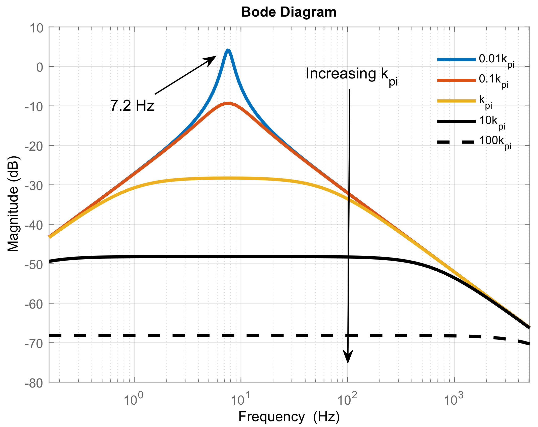
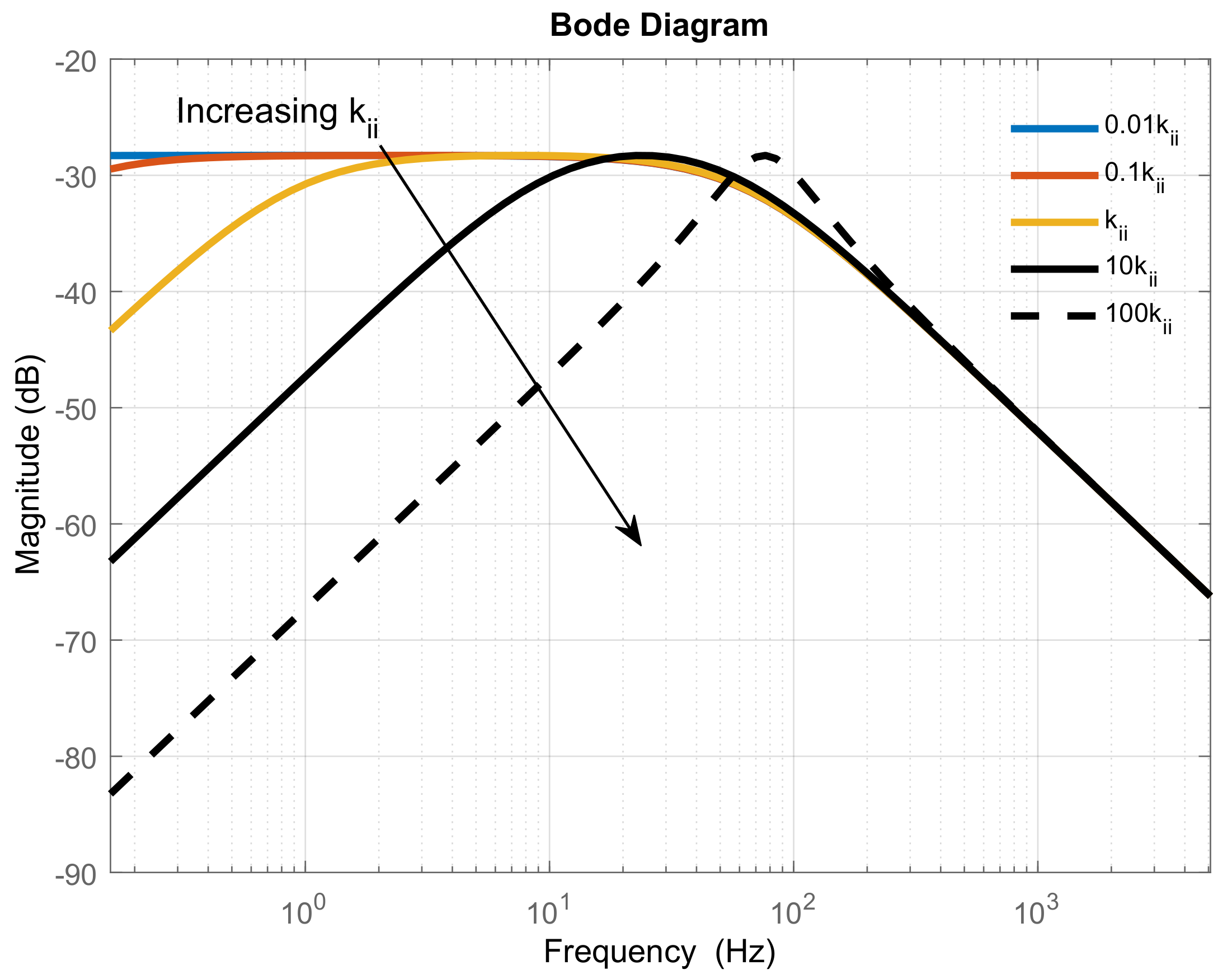
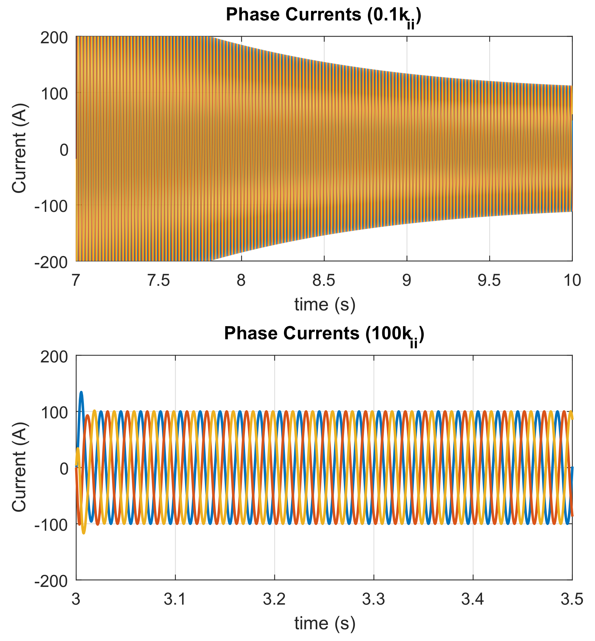
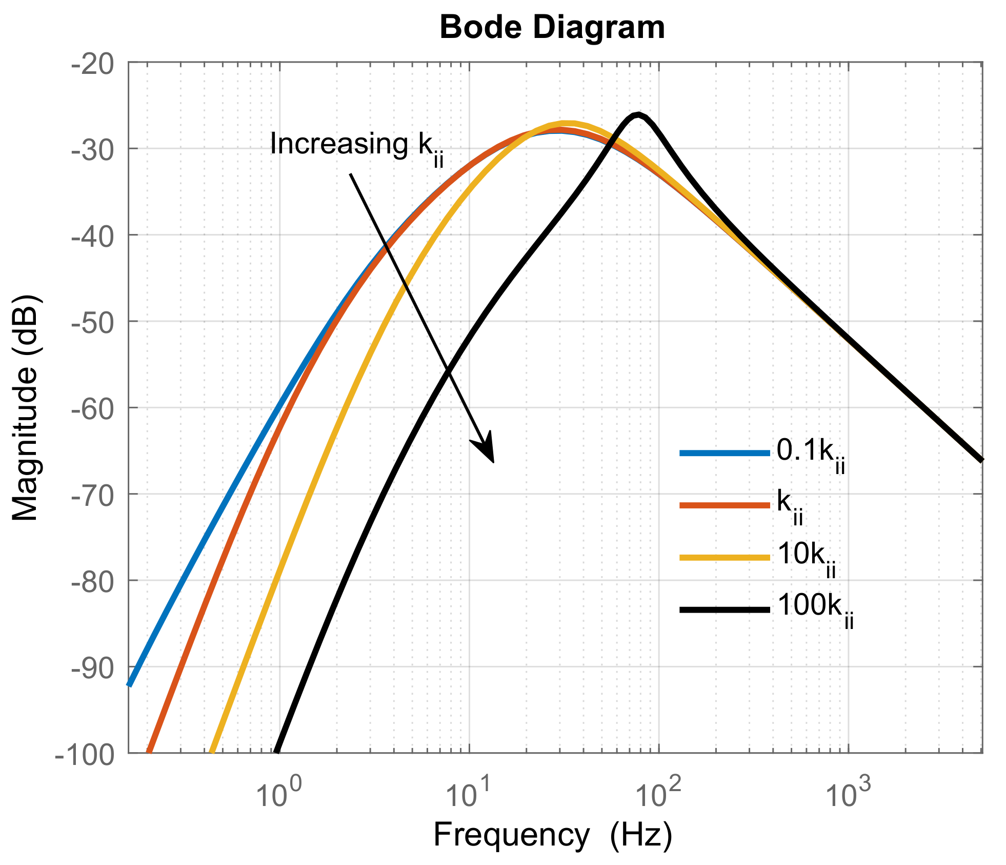
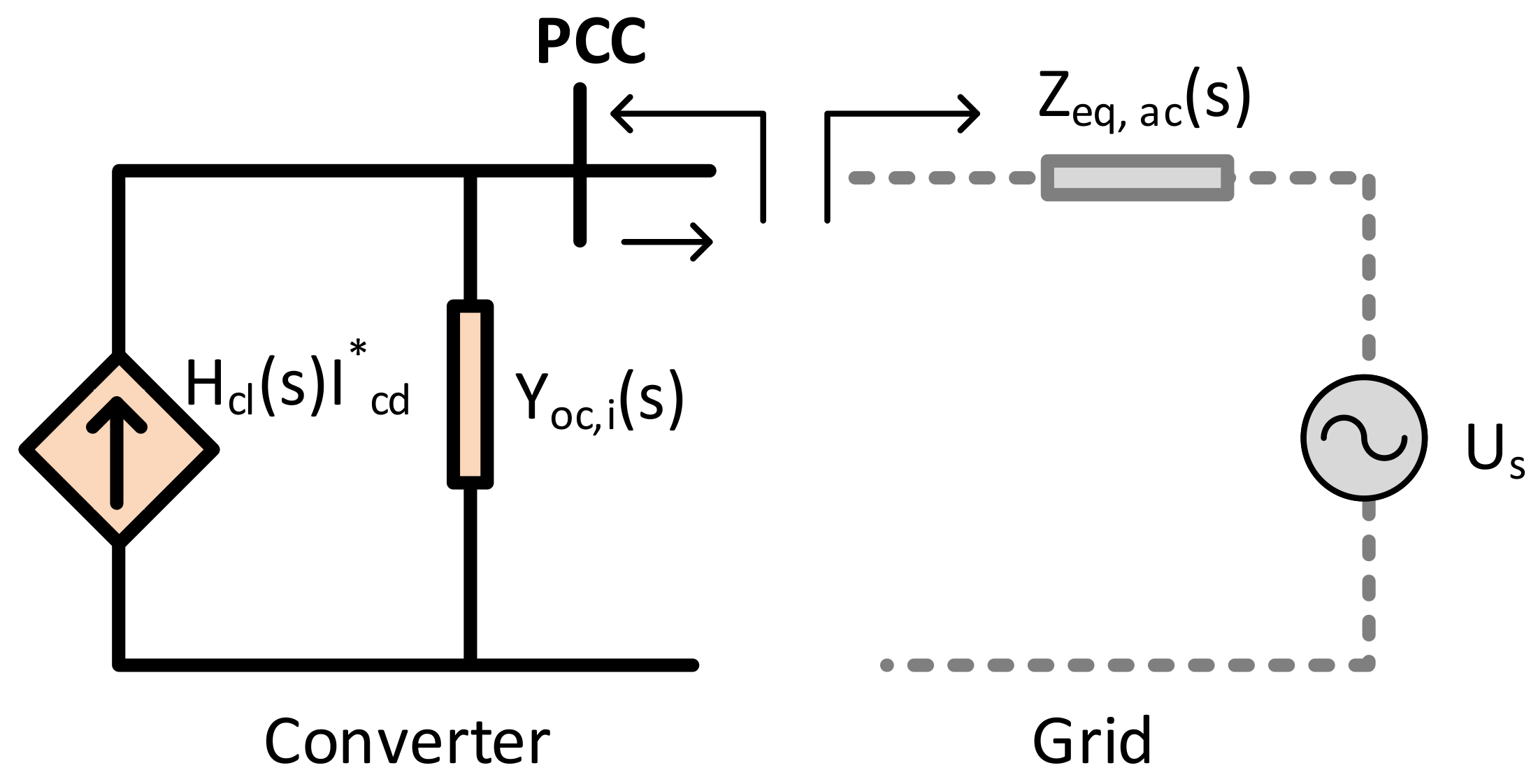
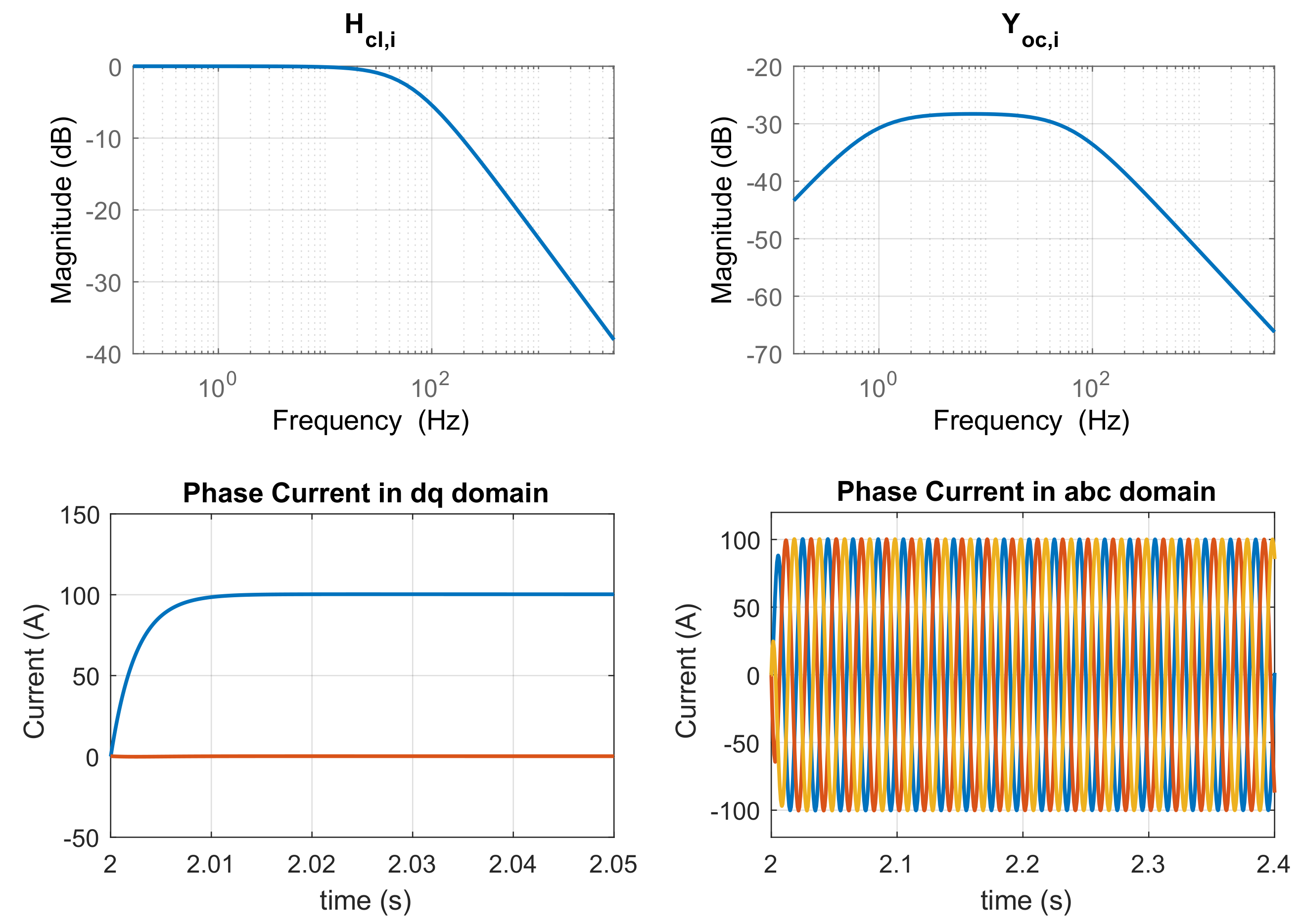
4.1.1. Output Admittance with Current Control Loop

Figure 11 depicts the frequency response plot of the output admittance (without the DC voltage loop) to inner-loop proportional gain sensitivity. Clearly, the proportional gain based on internal model control behaves as a virtual damper. Ideally, to prevent the AC grid voltage from acting as a disturbance, it is required that Y o c , i ( s ) is as low as possible. However, k p i cannot be infinitely increased as this would result to chaotic oscillations in AC voltage, which was assumed to be perfect. However, it should be noted that Y o c , i ( s ) also depends on the sensitivity function of the control system S ( s ) . Therefore, any means to obtain controller gains by minimizing Y o c , i ( s ) must also consider the closed-loop transfer function. Figure 12 depicts the time domain plot of the AC currents in the a b c domain for the first case with 0 . 01 × k p i and the base case. The case with 0 . 01 × k p i shows a resonance at a frequency matching that was obtained from the frequency response plot of the output admittance in Figure 11.
A similar sensitivity analysis was carried out for the integral gain as depicted in the frequency response plot in Figure 13. In general, the integral gain has no influence on harmonic resonance as can be observed from the plot, where the output admittance response remained negligibly low in all cases. However, the integral gain plays a role in control system performance, most importantly, reference tracking and settling time. Thus, the integral gain can be estimated based on best tracking response. On the contrary, as integral gain is increased substantially, integral gain induced oscillations start to appear. The time domain plot in Figure 14 shows that the integral plays little role in resonances for reasonable values. However, too low integral gain leads to very poor steady-state tracking.

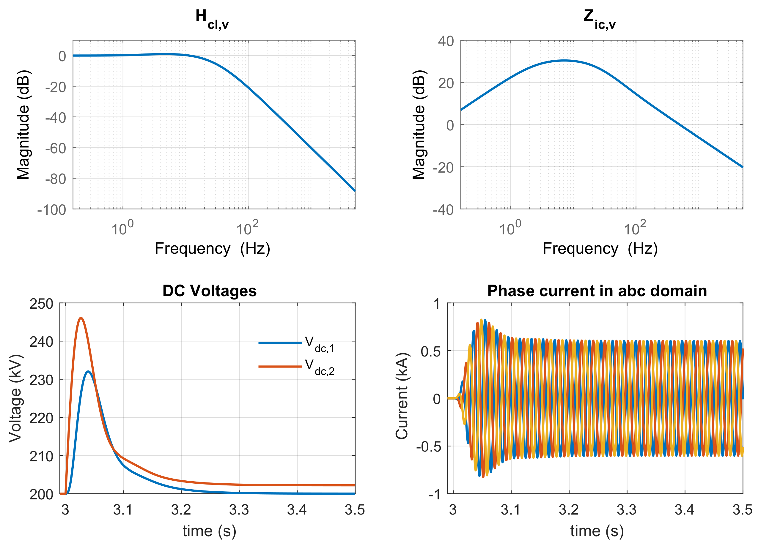
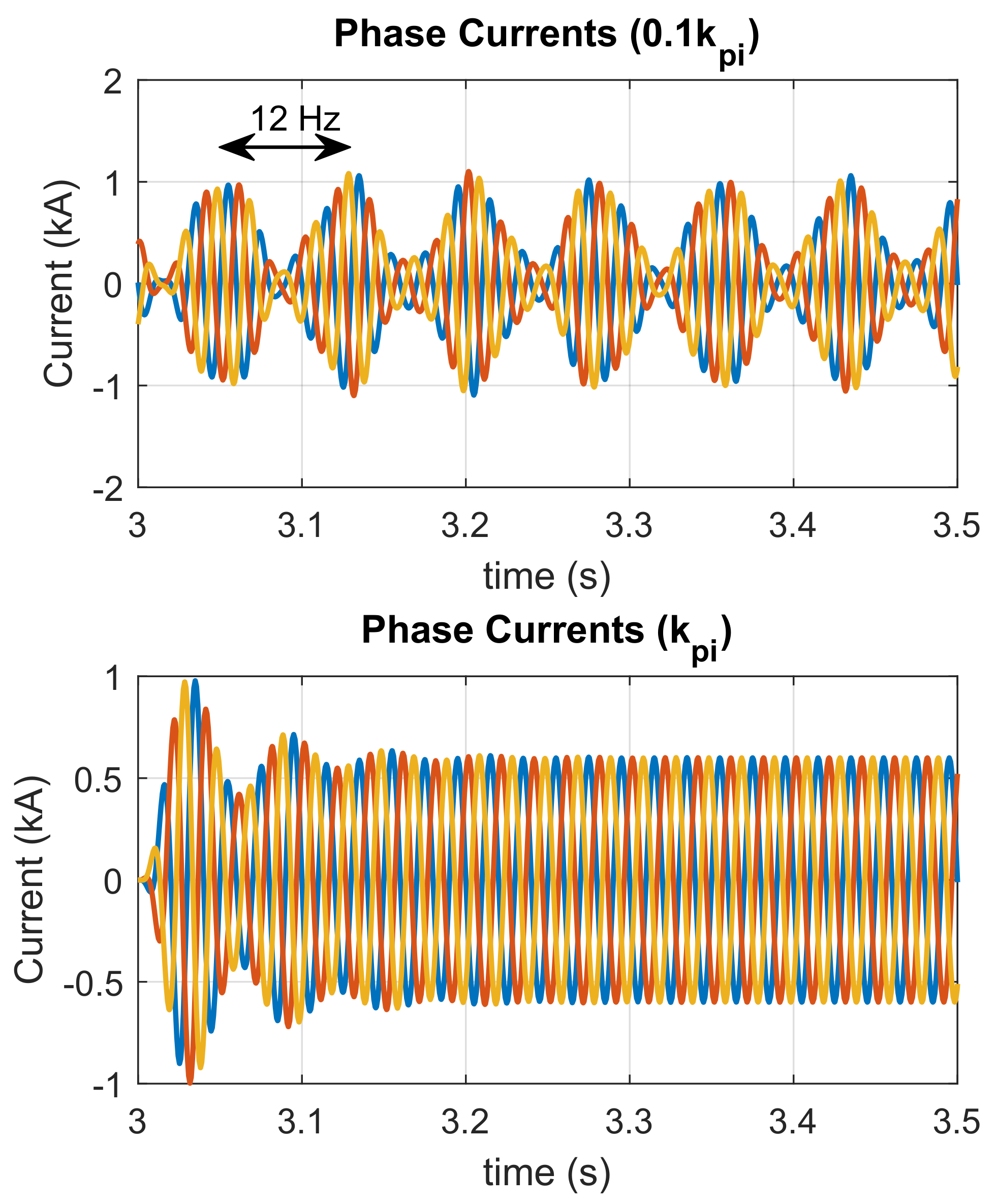
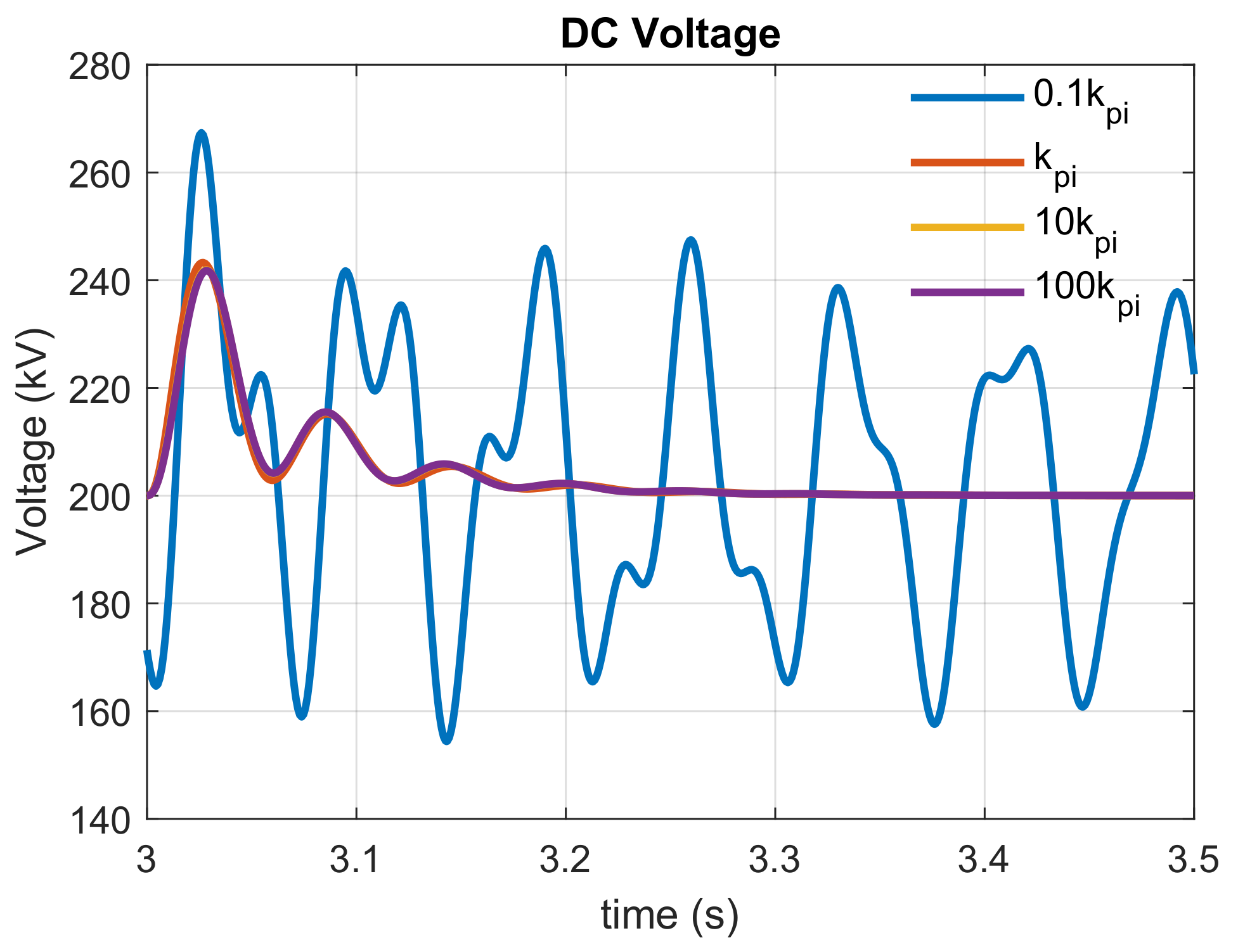
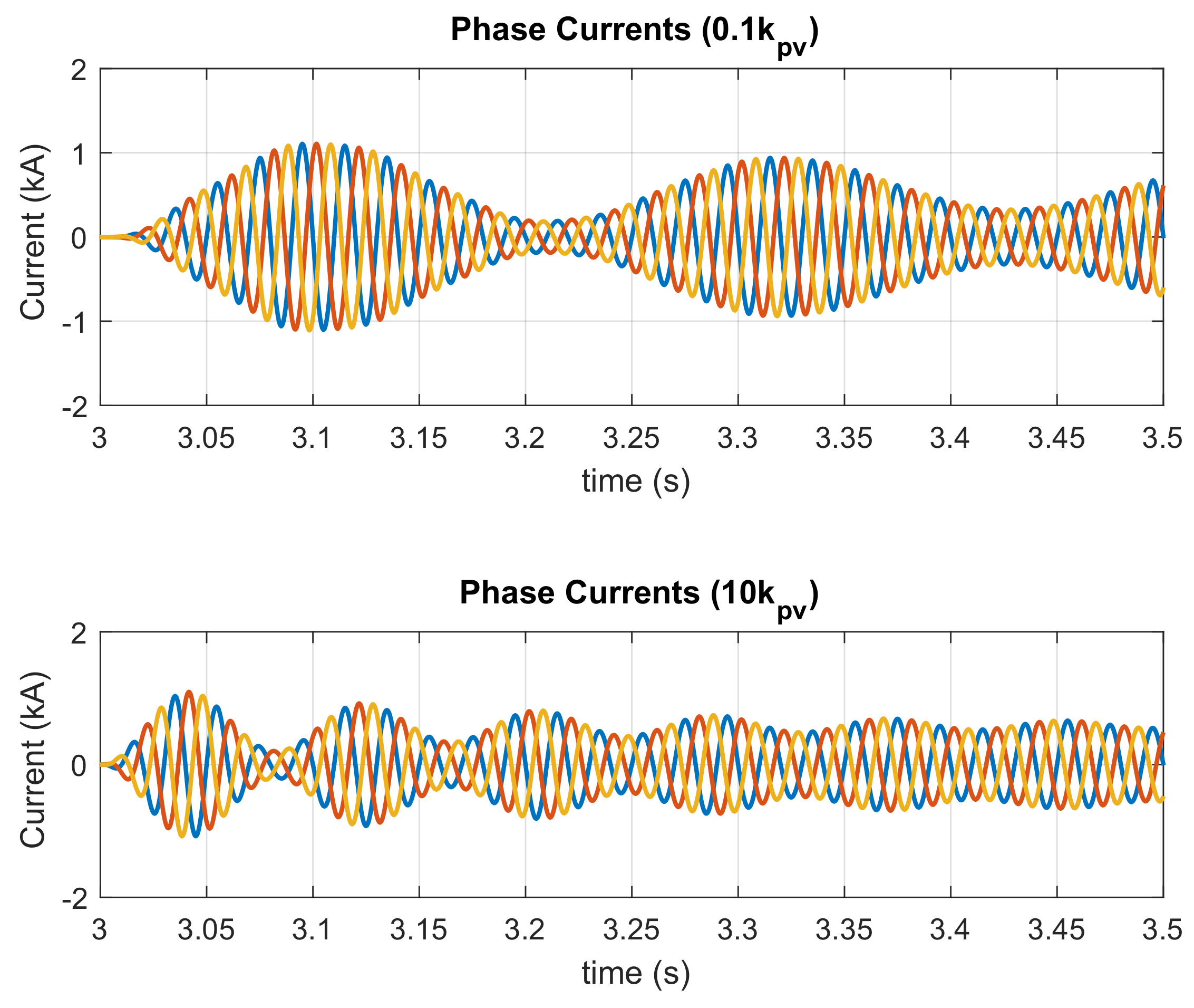
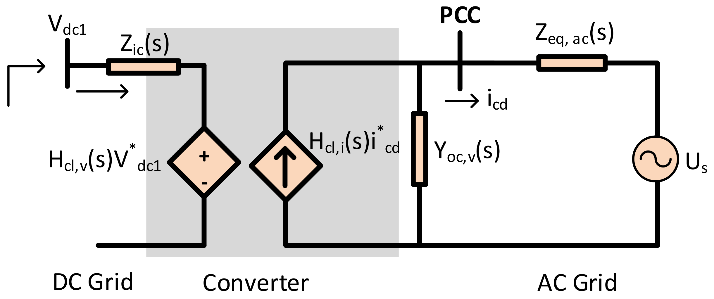
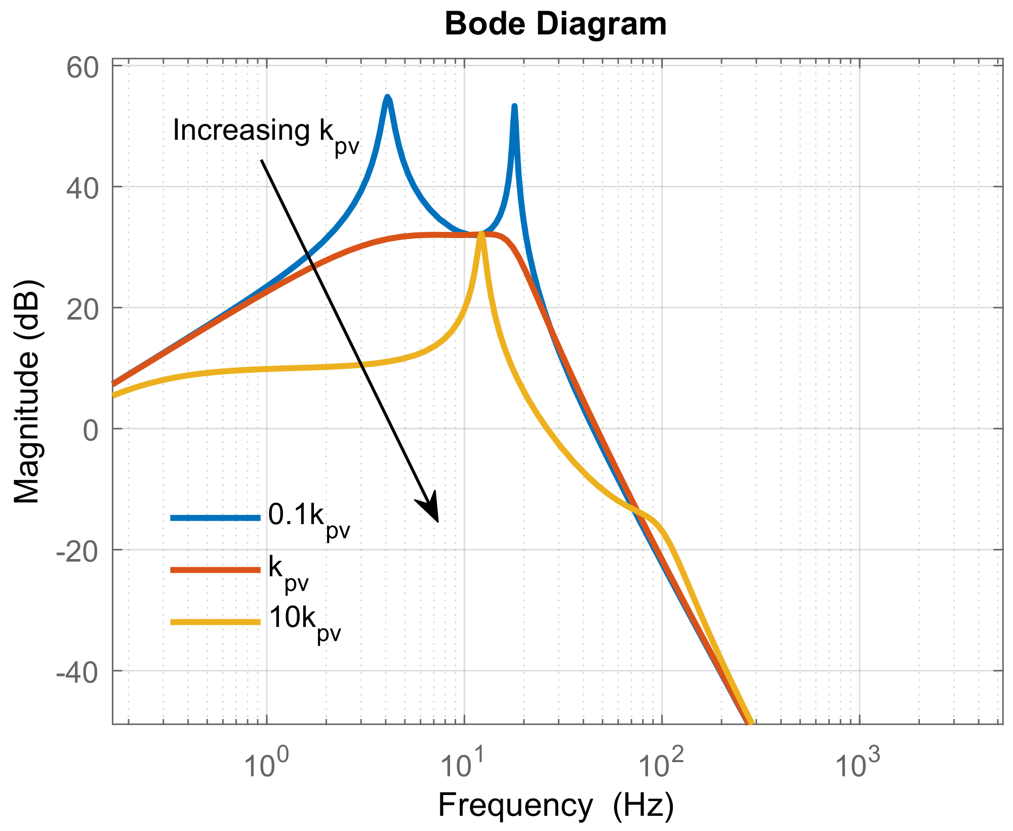
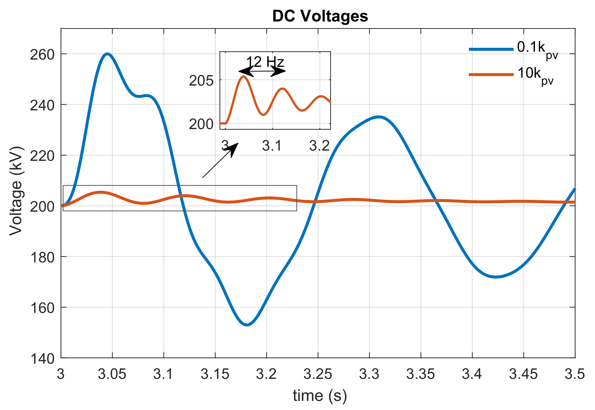
4.1.2. Output Admittance with DC Voltage Control Loop

This section details the sensitivity analysis of derived theoretical impedances due to the inclusion of the DC grid dynamics and DC voltage control loop. The DC voltage loop is in part influenced by the AC inner-loop and vice versa and this is of interest in the event that the converter is bidirectional. Additionally, the DC grid dynamics results in an input impedance as derived in (16). Both the AC output admittance and the DC input impedance provide information about resonances and possible instabilities on both sides of the converter.
Figure 15 depicts the plot of sensitivity of the output admittance due to DC voltage loop to variation in proportional gain of the inner controller. As depicted, a low proportional gain of the AC controller results in a resonance around 12 Hz. However, compared to the plot of output admittance with an AC inner-loop depicted in Figure 11, red plot, for the same parameter, the resonance magnitude is lower and the frequency is around 7 . 2 Hz. This clearly shows a remarkable difference between assuming a constant DC voltage, i.e., DC grid and voltage dynamics are ignored, and including the said dynamics. Figure 16 depicts the frequency response of the DC input impedance to k p i sensitivity, showing a similar resonance point as the output admittance Y o c , v . It also shows that the influence of k p i gain diminishes beyond the stable case as the responses almost match. Time domain plot of phase current in Figure 17 (top plot) shows the resonance with a matching frequency. However, beyond the base case value, k p i , the influence of AC inner-loop proportional gain on AC resonance diminishes as overall admittance remains negligibly low without resonance points. This shows the benefits of applying IMC principle in obtaining a perfect AC current compensator.
Figure 18 depicts the time domain plot of the DC voltages of grid side converter with time domain response matching the frequency response in Figure 16. It also shows that beyond the base case, k p i gain plays no role on the DC side response, as plot of DC voltages are similar.
Similarly, for the integral gain of inner-loop, no influence on resonance was observed, as depicted in Figure 19; however, the integral gain still plays a role in steady-state tracking performance. The same applies to the DC voltages shown in Figure 20.
Figure 21 depicts the frequency response of the output admittance with DC dynamics. For low values of k p v , resonances are prevalent. This is further observed in the time domain plot of Figure 22. Figure 23 depicts the time domain plot for the DC voltages. Contrary to expectations, above the base case, resonances are also observed. This establishes that the proportional gain cannot be increased infinitely degrading responses. A possible explanation for this is that at a DC voltage loop gain, the time response of the outer-loop becomes as fast, or even faster than the inner-loop, leading to interactions, resonances, and instabilities.
The integral gain of the outer-loop, k i v behaves similarly to that of inner-loop by having an insignificant impact on resonances. However, the integral gain is required for control system performance, particularly steady-state tracking. Thus, it cannot be completely disregarded.

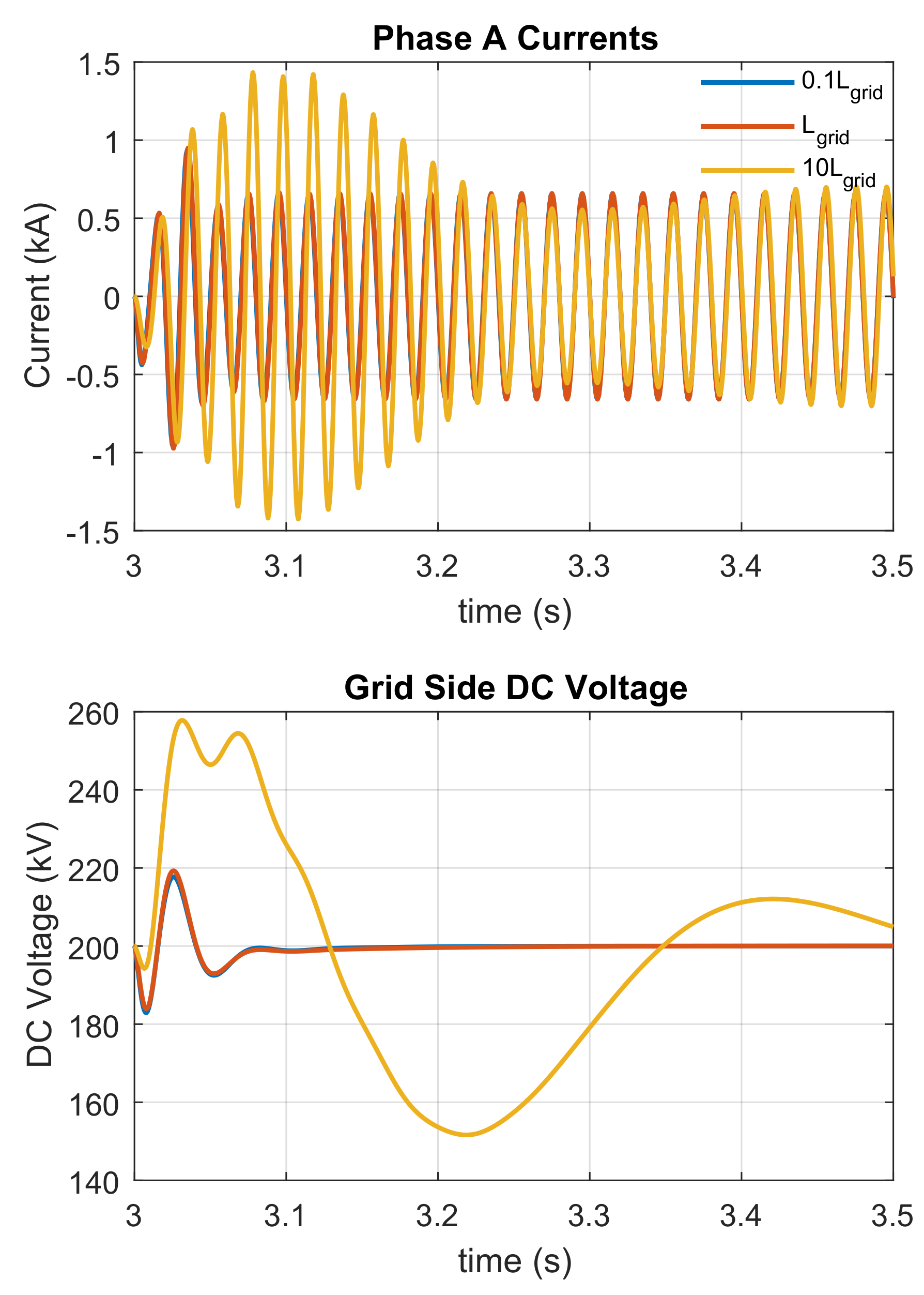
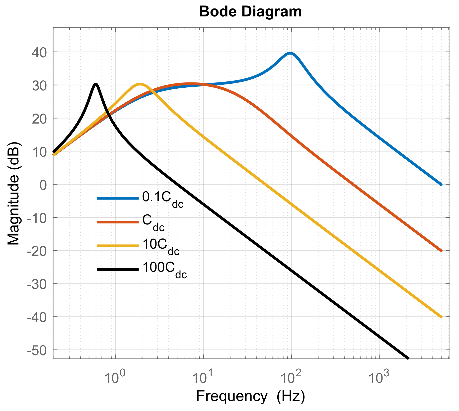
4.2. DC Grid Parameters

In this subsection, the impact of DC grid and its components on dynamic responses are studied. It has been shown from derivations that some dynamics from these components are transferred to the AC grid. An advantage of the theoretical procedure detailed in Section 3 is the capability to see from equations how components interact. From derived equations, the receiving terminal ‘sees’ the total sum of all capacitances directly connected to it. That is, for the HVDC link, equivalent capacitances at the receiving terminal C 1 and, similarly, C 2 at the sending terminal reflects as ( C 1 + C 2 ) at the receiving end. This implies that the receiving terminal sees some dynamics from the sending terminal.
Subsequent to this, the DC bus capacitances are varied (cable capacitance was kept constant as cable distance was not varied). Figure 24 shows the frequency response of the DC input impedance to varying bus capacitances. For increasing total DC capacitance, resonance magnitude slightly decreases. However, frequency of oscillations also moves to the low frequency region, and second resonant points at the low frequency region start to appear as total capacitance is significantly increased. Particularly, such low frequency oscillations (<2 Hz) result in sustained oscillations that are difficult to detect as they are also of low magnitude, whereas, with lower capacitances, resonances are of higher frequency and magnitude; however, they damp out fast (behaving more like impulse disturbances). Figure 25 depicts the time domain plot of DC voltages with varying capacitances.
Suffice to say, the influence of varying capacitances can be observed in AC side responses. This represents a compromise that must be made, but caution must be applied as this affects both the AC and DC grids and DC voltage oscillations may potentially transfer from one terminal to the other, influencing control efforts. It will be interesting to see how multi-terminal DC grids with increased capacitance will influence low frequency oscillations in the connected AC grid.

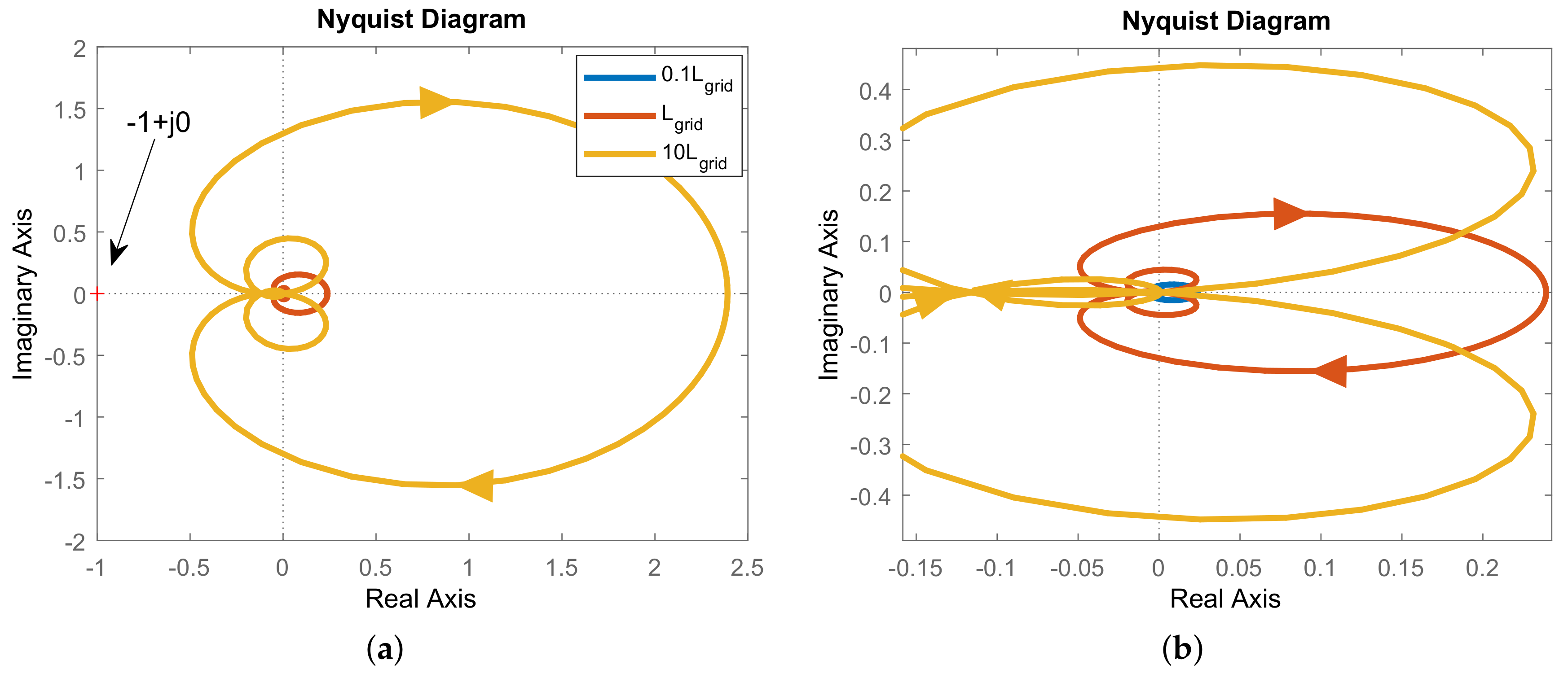
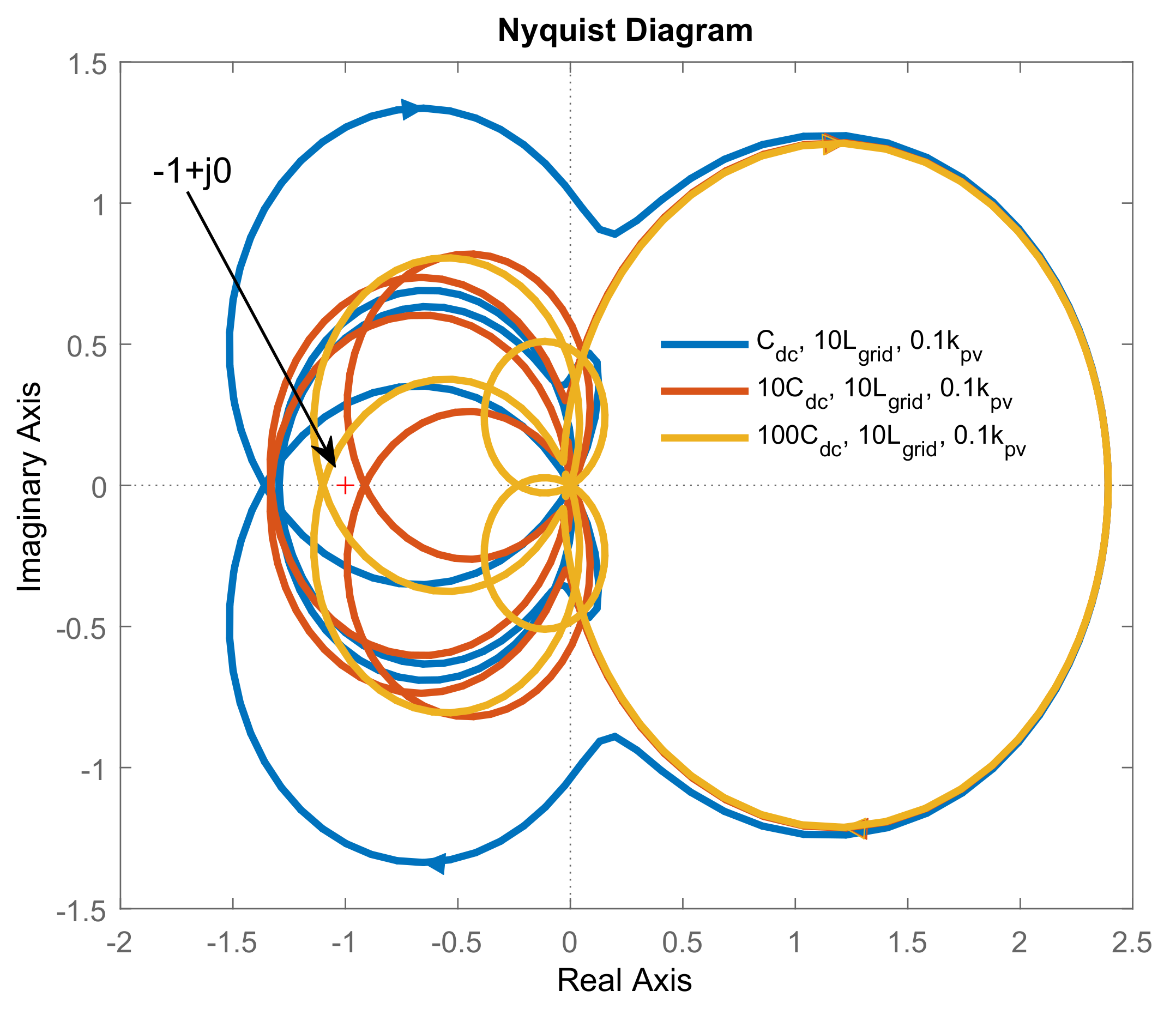
4.3. Harmonic Stability

Harmonic stability of the entire system on connection to a simplified AC grid (i.e., defined by inductive impedance) of defined short circuit ratio (SCR) and the DC link is carried out based on derivations in Section 3.3.
Figure 26 shows the Nyquist plot of sensitivity with varying SCR with the same base data. Clearly, the system maintains stability for a realistic range of SCRs. As time domain plots of Figure 27 depicts, although the system remains relatively stable, resonances and oscillations start to develop as SCR reduces. Any reduction in SCR, change in DC grid, or controller parameter may lead to instability.
To show this, stability sensitivity is carried out with a reduced SCR ( 10 L g r i d ), with reduced proportional gain of the outer controller ( 0 . 1 k p v ), and varying total capacitance of the DC side ( C D C ). Figure 28 depicts the Nyquist plot for increasing DC capacitance. As can be clearly seen, the system is unstable for all three cases, despite the controller being stable for each case. However, as capacitance is increased, the system moves closer to the stable region.

5. Conclusions

This paper has presented a parametric sensitivity analysis for resonance and stability performance of an integrated AC grid VSC-HVDC link system. This study has been carried out through the development of the impedance-based model of the entire electrical system (both DC and AC sides) and the converter controls in frequency domain. From the sensitivity analysis, it can be concluded that the control design parameters and and grid to be connected must be considered to ensure stability and avoid undesired dynamics. In addition, it is worth noting that, from the controller side, the proportional gain of the controller acts as a damper, in a similar way as resistance. On the other hand, the integral gain does not have great impact, but it is required to achieve steady state accuracy. Additionally, from the electrical component point of view, it can be seen that, with changing impedance response, there is a shift and change on the natural frequencies of the system, which may result in grid resonances, some of which are at the sub-synchronous level and even very low frequency regions. Finally, it is worth remarking that the grid impedance of the whole system plays a key role in the stability of the grid. Thus, this is crucial to develop the grid and controllers carefully since the impedance of grids with high penetration of power electronics is variable and dependent on current state, control, lines, etc.

Acknowledgments

This work was partially supported by the European Union’s Horizon 2020 research and innovation programme under Maria-Sklodowska-Curie action INCITE—“Innovative controls for renewable source integration into smart energy systems” (Grant agreement No. 675318). The work of J.L. Domínguez-García was also supported by the CERCA Programme from the Generalitat de Catalunya.

Author Contributions

Adedotun J. Agbemuko developed the analysis and the results. José Luis Domínguez-García and Eduardo Prieto-Araujo supported the modelling, simulation of the results, and reviewed the paper. Oriol Gomis-Bellmunt reviewed the contributions, results and papers.

Conflicts of Interest

The authors declare no conflict of interest.

Nomenclature

CConstant
G d Modulation delay
H A C / D C Closed-loop gain of AC to DC side of converter
H c l , i Closed-loop transfer functions from output to reference of current loop
H c l , v Closed-loop transfer functions from output to reference of DC voltage loop
H o l , i Open-loop gain of current loop
H o l , v Open-loop gain of DC voltage loop
I * Reference current
i c , a b c Converter AC current in abc frame
i c , d q Converter AC current in dq frame
I D C , n DC current injection at nth terminal
K c Current compensator
K i i Integral gain of current compensator
K i v Integral gain of DC voltage compensator
K p i Proportional gain of current compensator
K p v Proportional gain of DC voltage compensator
K v DC voltage compensator
L D C , c a b Inductance of DC cable
L f Inductance of filter
L t Inductance of transformer
P a c AC active power
P D C DC power
R t Transformer resistance
τ d Modulation delay
τ d Inner-loop time constant
U c , d q Converter AC voltage in dq frame
U c , a b c Converter AC voltage in abc frame
U s , d q Source AC voltage in dq frame
U s , a b c Source AC voltage in abc frame
V * DC voltage reference
V D C , n DC voltage at nth terminal
Y c Current compensator
Y o c , i Converter closed-loop output admittance with current loop
Y o c , v Converter closed-loop output admittance considering influence of DC voltage loop
Y s Admittance as seen from source
Z b u s , D C DC nodal impedance matrix
Z c f Filter capacitor impedance
Z c n Impedance of total DC capacitance at nth terminal
Z D C , c a b Impedance of DC cable
Z f Impedance of filter inductor
Z g , e q Equivalent AC grid impedance
Z i c Converter DC input impedance
Z o c , v Converter closed-loop output impedance considering influence of DC voltage loop
Z t Impedance of transformer

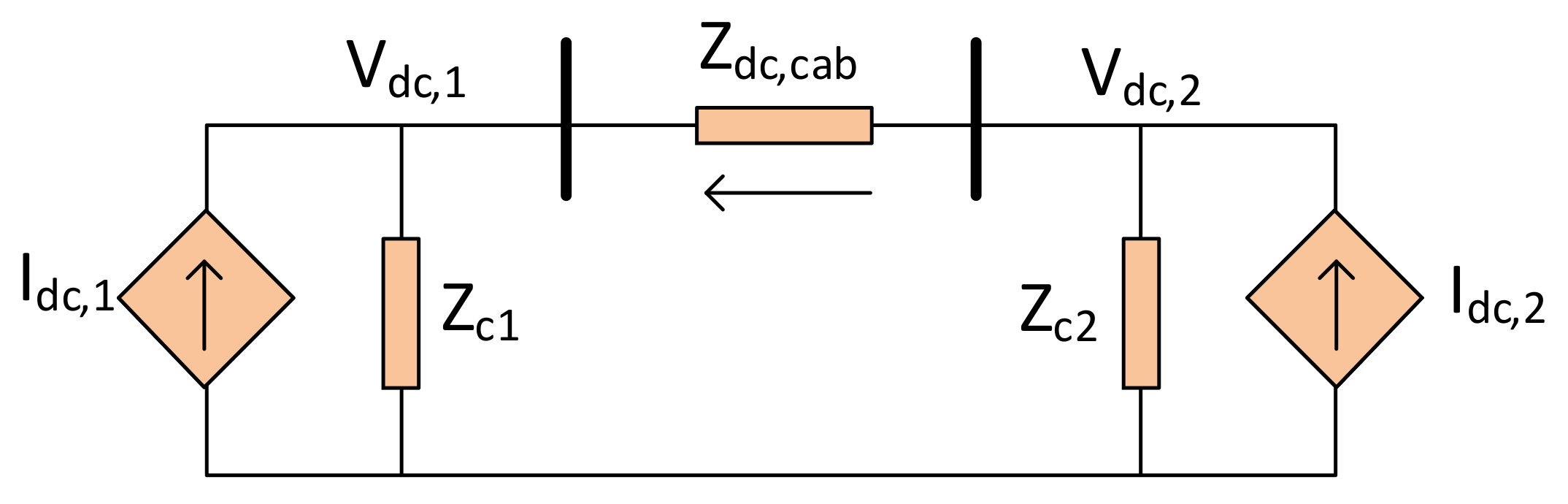
Appendix A. DC Voltage Equation of the HVDC Link

Consider circuit schematics of the HVDC link based on known nodal current injection as depicted in Figure A1. Following the current directions of the sources and arbitrary cable direction from terminal 2 to 1 as indicated, the aim is to obtain the dynamics of the nodal voltages, V D C , 1 and V D C , 2 . Apply KCL to each of terminals 1 and 2,
I D C , 1 = I c 1 - I c a b , I D C , 2 = I c 2 + I c a b ,
where Z c 1 , Z c 2 , Z D C , c a b are the terminal capacitors’ impedances and cable, respectively. I c 1 and I c 2 are the capacitor currents, and I c a b the DC cable current. Applying Ohm’s law to express branch currents in terms of nodal voltages,
I D C , 1 = V D C , 1 Z c 1 - V D C , 2 - V D C , 1 Z D C , c a b , I D C , 2 = V D C , 2 Z c 2 + V D C , 2 - V D C , 1 Z D C , c a b ,
from (A2),
I D C , 1 = V D C , 1 Z c 1 + V D C , 1 Z D C , c a b - V D C , 2 Z D C , c a b , I D C , 1 = V D C , 1 ( Z c 1 + Z D C , c a b ) Z c 1 Z D C , c a b - V D C , 2 Z D C , c a b ,
similarly for I D C , 2 ,
I D C , 2 = - V D C , 1 Z D C , c a b + V D C , 2 ( Z c 2 + Z D C , c a b ) Z c 2 Z D C , c a b
in matrix form, (A3) and (A4) can be written as,
I D C , 1 I D C , 2 = Z c 1 + Z D C , c a b Z c 1 Z D C , c a b - 1 Z D C , c a b - 1 Z D C , c a b Z c 2 + Z D C , c a b Z c 2 Z D C , c a b Y b u s D C ( s ) V D C , 1 V D C , 2 ,
since the nodal currents injection are known,
V D C , 1 V D C , 2 = Z c 1 + Z D C , c a b Z c 1 Z D C , c a b - 1 Z D C , c a b - 1 Z D C , c a b Z c 2 + Z D C , c a b Z c 2 Z D C , c a b - 1 I D C , 1 I D C , 2 . V D C , 1 V D C , 2 = Z c 1 ( Z c 2 + Z D C , c a b ) Z c 1 + Z D C , c a b + Z c 2 Z c 1 Z c 2 Z c 1 + Z D C , c a b + Z c 2 Z c 1 Z c 2 Z c 1 + Z D C , c a b + Z c 2 Z c 2 ( Z c 1 + Z D C , c a b ) Z c 1 + Z D C , c a b + Z c 2 I D C , 1 I D C , 2 .
In compact notation, the DC voltage dynamics can be derived as
V D C , 1 V D C , 2 = Z 11 ( s ) Z 12 ( s ) Z 21 ( s ) Z 22 ( s ) Z b u s D C ( s ) I D C , 1 I D C , 2 .
Figure A1. Circuit schematic of the HVDC link based on nodal current injection.
Energies 11 00845 g0a1

Appendix B. Transfer Functions

  • AC admittance with inner-loop
    Y o c , i ( s ) = Z c f Z t Z c f + Z t Z f + Z c f Z f + K c G d ( Z t + Z c f ) ,
    where Z c f = 1 / s C f , Z t = R t + s L t , Z f = s L f , K c = k p i + k i i / s , G d = 1 / ( τ d s + 1 ) .
  • Closed-loop transfer function of the inner-loop,
    H c l , i ( s ) = K c G d ( Z t + Z c f ) Z t Z c f + Z t Z f + Z c f Z f + K c G d ( Z t + Z c f ) .
  • Open-loop transfer function of the complete system,
    H o l , v ( s ) = A 3 A 4 Z c 1 ( Z D C , c a b + Z c 2 ) ( A 0 + A 1 + A 2 + A 3 ) ( Z c 1 + Z D C , c a b + Z c 2 ) ,
    where
    A 0 ( s ) = Z t ( s ) Z c f ( s ) ,
    A 1 ( s ) = Z t ( s ) Z f ( s ) ,
    A 2 ( s ) = Z f ( s ) Z c f ( s ) ,
    A 3 ( s ) = K c ( s ) G d ( s ) ( Z t ( s ) + Z c f ( s ) ) ,
    A 4 ( s ) = K K v ( s ) ,
    where K v ( s ) = k p v + k i v / s .
  • Closed-loop transfer function of the complete system,
    H c l , v ( s ) = A 3 A 4 B 1 B 0 ( A 0 + A 1 + A 2 + A 3 ) + A 3 A 4 B 1 ,
    where
    B 0 ( s ) = Z c 1 ( s ) + Z D C , c a b ( s ) + Z c 2 ( s ) ,
    B 1 ( s ) = Z c 1 ( s ) ( Z D C , c a b ( s ) + Z c 2 ( s ) ) .
  • AC admittance with complete system,
    Y o c , v ( s ) = Z c f B 0 B 0 ( A 0 + A 1 + A 2 + A 3 ) + A 3 A 4 B 1 ,
  • DC impedance with complete system,
    Z i c , v ( s ) = Z c 1 Z c 2 ( A 0 + A 1 + A 2 + A 3 ) B 0 ( A 0 + A 1 + A 2 + A 3 ) + A 3 A 4 B 1 ,
  • Characteristic equation of the entire system,
    B 0 ( A 0 + A 1 + A 2 + A 3 ) + A 3 A 4 B 1 = 0 .
Table A1. Grid data for system understudy.
ParameterValue
Base Power800 MVA
AC Voltage220 kV
DC Voltage200 kV
Frequency50 Hz
DC Cable Length200 km
L t 35 mH
R t 0.363 Ω
L f 29 mH
C f 10–100 μ F
Z g r i d 4.813 Ω
Table A2. Control data.
Control DataValue
k p i 25.6
k i i 145.2
k p v 0.0192
k i v 0.272

References

  1. European Wind Energy Association. EU Energy Policy to 2050: Achieving 80–95% Emissions Reductions; EWEA: Brussels, Belgium, 2011. [Google Scholar]
  2. Meyer, C.; Hoing, M.; Peterson, A.; Doncker, R.W.D. Control and Design of DC Grids for Offshore Wind Farms. IEEE Trans. Ind. Appl. 2007, 43, 1475–1482. [Google Scholar] [CrossRef]
  3. Yazdani, A.; Iravani, R. Voltage-Sourced Converters in Power Systems: Modeling, Control, and Applications; John Wiley & Sons: Hoboken, NJ, USA, 2010. [Google Scholar]
  4. Dierckxsens, C.; Srivastava, K.; Reza, M.; Cole, S.; Beerten, J.; Belmans, R. A distributed DC voltage control method for VSC-MTDC systems. Electr. Power Syst. Res. 2012, 82, 54–58. [Google Scholar] [CrossRef]
  5. Yang, S.; Bryant, A.; Mawby, P.; Xiang, D.; Ran, L.; Tavner, P. An Industry-Based Survey of Reliability in Power Electronic Converters. IEEE Trans. Ind. Appl. 2011, 47, 1441–1451. [Google Scholar] [CrossRef]
  6. Wang, H.; Liserre, M.; Blaabjerg, F. Toward Reliable Power Electronics: Challenges, Design Tools, and Opportunities. IEEE Ind. Electron. Mag. 2013, 7, 17–26. [Google Scholar] [CrossRef]
  7. Liserre, M.; Teodorescu, R.; Blaabjerg, F. Stability of photovoltaic and wind turbine grid-connected inverters for a large set of grid impedance values. IEEE Trans. Power Electron. 2006, 21, 263–272. [Google Scholar] [CrossRef]
  8. Enslin, J.H.R.; Heskes, P.J.M. Harmonic interaction between a large number of distributed power inverters and the distribution network. IEEE Trans. Power Electron. 2004, 19, 1586–1593. [Google Scholar] [CrossRef]
  9. Wang, X.; Blaabjerg, F.; Loh, P.C. Proportional derivative based stabilizing control of paralleled grid converters with cables in renwable power plants. In Proceedings of the 2014 IEEE Energy Conversion Congress and Exposition (ECCE), Pittsburgh, PA, USA, 14–18 September 2014; pp. 4917–4924. [Google Scholar]
  10. Céspedes, M.; Sun, J. Impedance shaping of three-phase grid-parallel voltage-source converters. In Proceedings of the 2012 Twenty-Seventh Annual IEEE Applied Power Electronics Conference and Exposition (APEC), Orlando, FL, USA, 5–9 Feburary 2012; pp. 754–760. [Google Scholar]
  11. Harnefors, L.; Wang, X.; Yepes, A.G.; Blaabjerg, F. Passivity-Based Stability Assessment of Grid-Connected VSCs; An Overview. IEEE J. Emerg. Sel. Top. Power Electron. 2016, 4, 116–125. [Google Scholar] [CrossRef]
  12. Harnefors, L.; Zhang, L.; Bongiorno, M. Frequency-domain passivity-based current controller design. IET Power Electron. 2008, 1, 455–465. [Google Scholar] [CrossRef]
  13. Vesti, S.; Suntio, T.; Oliver, J.A.; Prieto, R.; Cobos, J.A. Impedance-Based Stability and Transient-Performance Assessment Applying Maximum Peak Criteria. IEEE Trans. Power Electron. 2013, 28, 2099–2104. [Google Scholar] [CrossRef]
  14. Sun, J. Small-Signal Methods for AC Distributed Power Systems—A Review. IEEE Trans. Power Electron. 2009, 24, 2545–2554. [Google Scholar]
  15. Sun, J. Impedance-Based Stability Criterion for Grid-Connected Inverters. IEEE Trans. Power Electron. 2011, 26, 3075–3078. [Google Scholar] [CrossRef]
  16. Chen, M.; Sun, J. Low-Frequency Input Impedance Modeling of Boost Single-Phase PFC Converters. IEEE Trans. Power Electron. 2007, 22, 1402–1409. [Google Scholar] [CrossRef]
  17. Yang, D.; Ruan, X.; Wu, H. Impedance Shaping of the Grid-Connected Inverter with LCL Filter to Improve Its Adaptability to the Weak Grid Condition. IEEE Trans. Power Electron. 2014, 29, 5795–5805. [Google Scholar] [CrossRef]
  18. Rygg, A.; Molinas, M.; Zhang, C.; Cai, X. On the Equivalence and Impact on Stability of Impedance Modeling of Power Electronic Converters in Different Domains. IEEE J. Emerg. Sel. Top. Power Electron. 2017, 5, 1444–1454. [Google Scholar] [CrossRef]
  19. Wang, X.; Harnefors, L.; Blaabjerg, F. Unified Impedance Model of Grid-Connected Voltage-Source Converters. IEEE Trans. Power Electron. 2018, 33, 1775–1787. [Google Scholar] [CrossRef]
  20. Cespedes, M.; Sun, J. Impedance Modeling and Analysis of Grid-Connected Voltage-Source Converters. IEEE Trans. Power Electron. 2014, 29, 1254–1261. [Google Scholar] [CrossRef]
  21. Harnefors, L.; Yepes, A.G.; Vidal, A.; Doval-Gandoy, J. Passivity-Based Controller Design of Grid-Connected VSCs for Prevention of Electrical Resonance Instability. IEEE Trans. Ind. Electron. 2015, 62, 702–710. [Google Scholar] [CrossRef]
  22. Jessen, L.; Fuchs, F.W. Modeling of inverter output impedance for stability analysis in combination with measured grid impedances. In Proceedings of the 2015 IEEE 6th International Symposium on Power Electronics for Distributed Generation Systems (PEDG), Aachen, Germany, 22–25 June 2015; pp. 1–7. [Google Scholar]
  23. Cho, Y.; Hur, K.; Kang, Y.C.; Muljadi, E. Impedance-Based Stability Analysis in Grid Interconnection Impact Study Owing to the Increased Adoption of Converter-Interfaced Generators. Energies 2017, 10, 1355. [Google Scholar] [CrossRef]
  24. Freijedo, F.D.; Chaudhary, S.K.; Teodorescu, R.; Guerrero, J.M.; Bak, C.L.; Kocewiak, H.; Jensen, C.F. Harmonic resonances in Wind Power Plants: Modeling, analysis and active mitigation methods. In Proceedings of the 2015 IEEE Eindhoven PowerTech, Eindhoven, The Netherlands, 29 June–2 July 2015; pp. 1–6. [Google Scholar]
  25. Liu, H.; Sun, J. Voltage Stability and Control of Offshore Wind Farms with AC Collection and HVDC Transmission. IEEE J. Emerg. Sel. Top. Power Electron. 2014, 2, 1181–1189. [Google Scholar]
  26. Amin, M.; Molinas, M. Understanding the Origin of Oscillatory Phenomena Observed between Wind Farms and HVDC Systems. IEEE J. Emerg. Sel. Top. Power Electron. 2017, 5, 378–392. [Google Scholar] [CrossRef]
  27. Ebrahimzadeh, E.; Blaabjerg, F.; Wang, X.; Bak, C.L. Efficient approach for harmonic resonance identification of large Wind Power Plants. In Proceedings of the 2016 IEEE 7th International Symposium on Power Electronics for Distributed Generation Systems (PEDG), Vancouver, BC, Canada, 27–30 June 2016; pp. 1–7. [Google Scholar]
  28. Kunjumuhammed, L.P.; Pal, B.C.; Oates, C.; Dyke, K.J. Electrical Oscillations in Wind Farm Systems: Analysis and Insight Based on Detailed Modeling. IEEE Trans. Sustain. Energy 2016, 7, 51–62. [Google Scholar] [CrossRef]
  29. Xu, L.; Fan, L. Impedance-Based Resonance Analysis in a VSC-HVDC System. IEEE Trans. Power Deliv. 2013, 28, 2209–2216. [Google Scholar] [CrossRef]
  30. Xu, L.; Fan, L.; Miao, Z. DC Impedance-Model-Based Resonance Analysis of a VSC-HVDC System. IEEE Trans. Power Deliv. 2015, 30, 1221–1230. [Google Scholar] [CrossRef]
  31. Pinares, G.; Bongiorno, M. Modeling and Analysis of VSC-Based HVDC Systems for DC Network Stability Studies. IEEE Trans. Power Deliv. 2016, 31, 848–856. [Google Scholar] [CrossRef]
  32. Agbemuko, A.J.; Domınguez-Garcıa, J.L.; Prieto-Araujo, E.; Gomis-Bellmunt, O. Harmonic Stability and Interactions in Meshed VSC-HVDC Dominated Power Systems. In Proceedings of the 16th International Wind Integration Workshop, Berlin, Germany, 25–27 October 2017. [Google Scholar]
  33. Zou, C.; GE, H.R.; Xu, S.; Li, Y.; Li, W.; Chen, J.; Zhao, X.; Yang, Y.; Lei, B. Analysis of Resonance between a VSC-HVDC Converter and the AC Grid. IEEE Trans. Power Electron. 2018. [Google Scholar] [CrossRef]
  34. Haileselassie, T.M.; Uhlen, K. Impact of DC Line Voltage Drops on Power Flow of MTDC Using Droop Control. IEEE Trans. Power Syst. 2012, 27, 1441–1449. [Google Scholar] [CrossRef]
  35. Harnefors, L.; Nee, H.P. Model-based current control of AC machines using the internal model control method. IEEE Trans. Ind. Appl. 1998, 34, 133–141. [Google Scholar] [CrossRef]
  36. Chaudhuri, N.; Chaudhuri, B.; Majumder, R.; Yazdani, A. Multi-Terminal Direct-Current Grids: Modeling, Analysis, and Control; John Wiley & Sons: Hoboken, NJ, USA, 2014. [Google Scholar]
  37. Wang, X.; Blaabjerg, F.; Wu, W. Modeling and Analysis of Harmonic Stability in an AC Power-Electronics-Based Power System. IEEE Trans. Power Electron. 2014, 29, 6421–6432. [Google Scholar] [CrossRef]
  38. Amin, M.; Molinas, M.; Lyu, J.; Cai, X. Impact of Power Flow Direction on the Stability of VSC-HVDC Seen From the Impedance Nyquist Plot. IEEE Trans. Power Electron. 2017, 32, 8204–8217. [Google Scholar] [CrossRef]
  39. Amin, M.; Rygg, A.; Molinas, M. Impedance-based and eigenvalue based stability assessment compared in VSC-HVDC system. In Proceedings of the 2016 IEEE Energy Conversion Congress and Exposition (ECCE), Milwaukee, WI, USA, 18–22 September 2016; pp. 1–8. [Google Scholar]
Figure 1. HVDC (High voltage direct current) point-to-point link.
Energies 11 00845 g001
Figure 2. HVDC impedance circuit and control architecture.
Energies 11 00845 g002
Figure 3. Inner current loop and physical grid.
Energies 11 00845 g003
Figure 4. Analytical block diagram of the d-axis current controller.
Energies 11 00845 g004
Figure 5. Equivalent circuit representation of current controller relative to the grid.
Energies 11 00845 g005
Figure 6. (Top left) Frequency response of closed-loop output to reference transfer function; (Top right) frequency response of output admittance with current control (base case); (Bottom left) time response of phase currents in the dq domain; (Bottom right) time response plot of phase currents in the abc domain for a step change to validate base case.
Energies 11 00845 g006
Figure 7. Control block diagram of the DC voltage control.
Energies 11 00845 g007
Figure 8. (Top left) Frequency response of closed-loop output to reference transfer function; (Top right) frequency response of input impedance from DC (base case); (Bottom left) time response of DC voltages; (Bottom right) time response plot of phase currents in abc domain.
Energies 11 00845 g008
Figure 9. Equivalent circuit representation of converter relative to the system.
Energies 11 00845 g009
Figure 10. Impedance model of converter and connected grid impedance.
Energies 11 00845 g010
Figure 11. Sensitivity of Output Admittance Y o c , i ( s ) to k p i in increasing order of 0 . 01 × , 0 . 1 × , 1 × , and= 10 × k p i (base case).
Energies 11 00845 g011
Figure 12. (Top plot) time domain plot of phase currents in a b c frame, showing sustained resonances for the case with 0 . 01 × k p i with a matching frequency with that of frequency response; (Bottom plot) base case with no resonance.
Energies 11 00845 g012
Figure 13. Sensitivity of Output Admittance Y o c , i ( s ) to k i i in increasing order of 0 . 01 × , 0 . 1 × , 1 × , 10 × , and 10 × k i i (base case).
Energies 11 00845 g013
Figure 14. (Top plot) time domain plot of phase currents in a b c frame, for the case with 0 . 01 × k i i showing poor steady-state accuracy; (Bottom plot) 100 × k i i .
Energies 11 00845 g014
Figure 15. Sensitivity of output admittance Y o c , v to k p i in increasing order of 0 . 1 × , 1 × , 10 × , and 100 × k p i (base case).
Energies 11 00845 g015
Figure 16. Sensitivity of DC input impedance to k p i in increasing order of 0 . 1 × , 1 × , 10 × , and 100 × k p i (base case).
Energies 11 00845 g016
Figure 17. (Top plot) time domain plot of phase currents in a b c frame, for the case with 0 . 1 × k p i showing resonances at around 12 Hz; (Bottom plot) base case with k p i .
Energies 11 00845 g017
Figure 18. Time domain plot of grid side DC voltage to sensitivity of inner-controller proportional gain, k p i .
Energies 11 00845 g018
Figure 19. Sensitivity of output admittance Y o c , v to k i i in increasing order of 0 . 1 × , 1 × , 10 × , and 100 × k i i (base case).
Energies 11 00845 g019
Figure 20. Time domain plot of grid side DC voltage to sensitivity of inner-controller integral gain, k i i .
Energies 11 00845 g020
Figure 21. Sensitivity of DC input Impedance Z i c to k p v in increasing order of 0.1×, 0 . 1 × , 1 × , and 10 × k p v (base case).
Energies 11 00845 g021
Figure 22. (Top plot) time domain plot of Phase AC currents in the abc frame for the case of 0 . 1 k p v ; (Bottom plot) case of 10 k p v .
Energies 11 00845 g022
Figure 23. Time domain plot of grid side DC voltage to sensitivity of outer-loop proportional gain, k p v .
Energies 11 00845 g023
Figure 24. Input impedance sensitivity to total DC capacitance with capacitances 0 . 1 × , 1 × , 10 × , 100 × C D C , b u s at both terminals, where C D C , b u s is the nominal bus capacitance of 300 μ F.
Energies 11 00845 g024
Figure 25. Time domain plot of grid side DC voltage varying DC capacitance.
Energies 11 00845 g025
Figure 26. Stability sensitivity to varying SCRs (short circuit ratios); (a) main plot; (b) zoomed plot.
Energies 11 00845 g026
Figure 27. (Top) Phase A currents for varying SCRs; (Bottom) grid side DC voltages for varying SCRs.
Energies 11 00845 g027
Figure 28. Stability sensitivity to varying DC grid capacitance.
Energies 11 00845 g028

