Scenario Analysis of Natural Gas Consumption in China Based on Wavelet Neural Network Optimized by Particle Swarm Optimization Algorithm

Abstract
:1. Introduction
2. Methodology
2.1. Particle Swarm Optimization (PSO)
| Algorithm 1 Pseudocode of PSO algorithm. |
| Begin Create the particle swarm and initialize particles repeat For all do Compute fitness of each particle If Replace Pbest by , i.e., End if If Replace Gbest by , i.e., End if Update the particles using the following two equations End for Until the termination condition is satisfied Output the best particle position End |
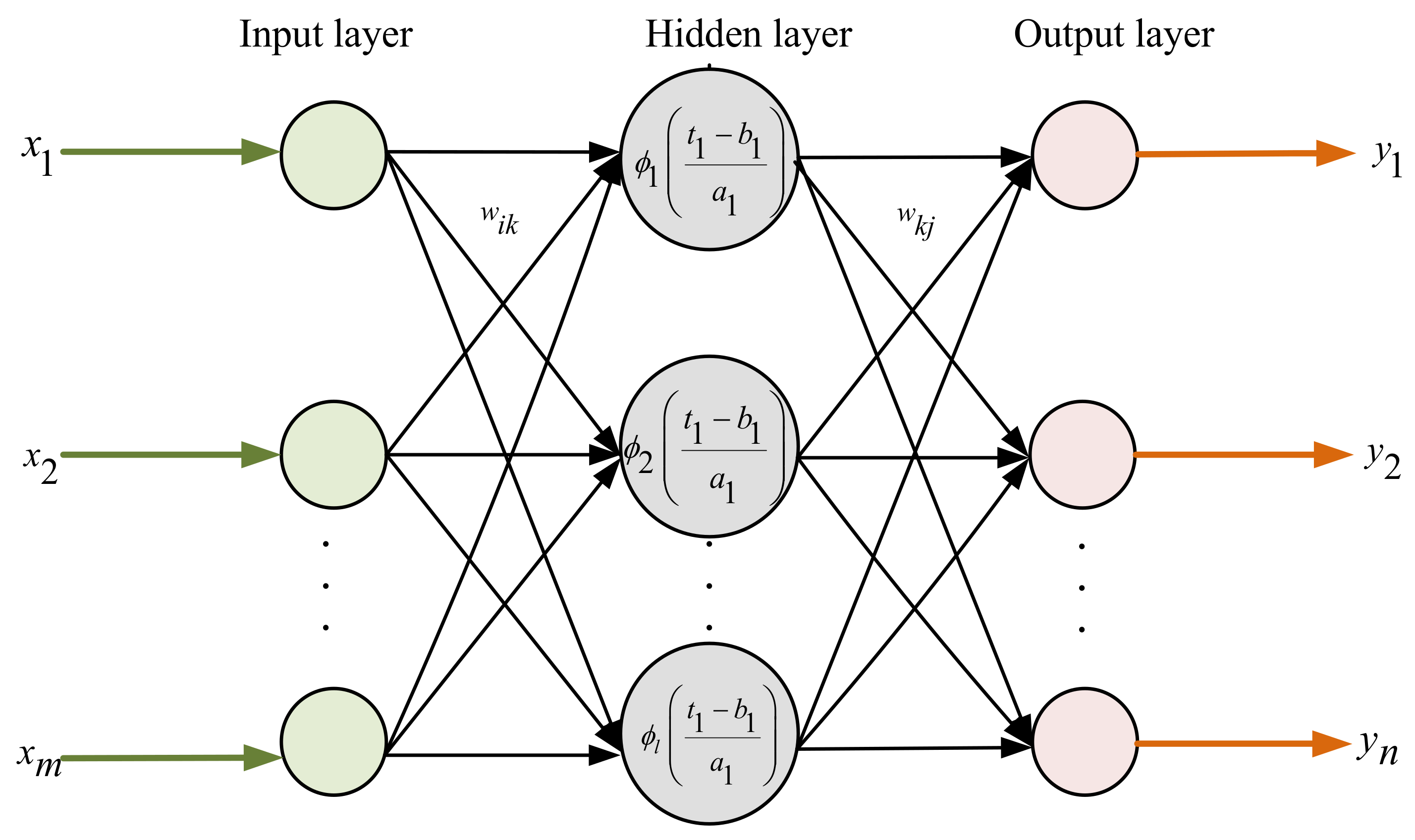
2.2. Wavelet Neural Network (WNN)
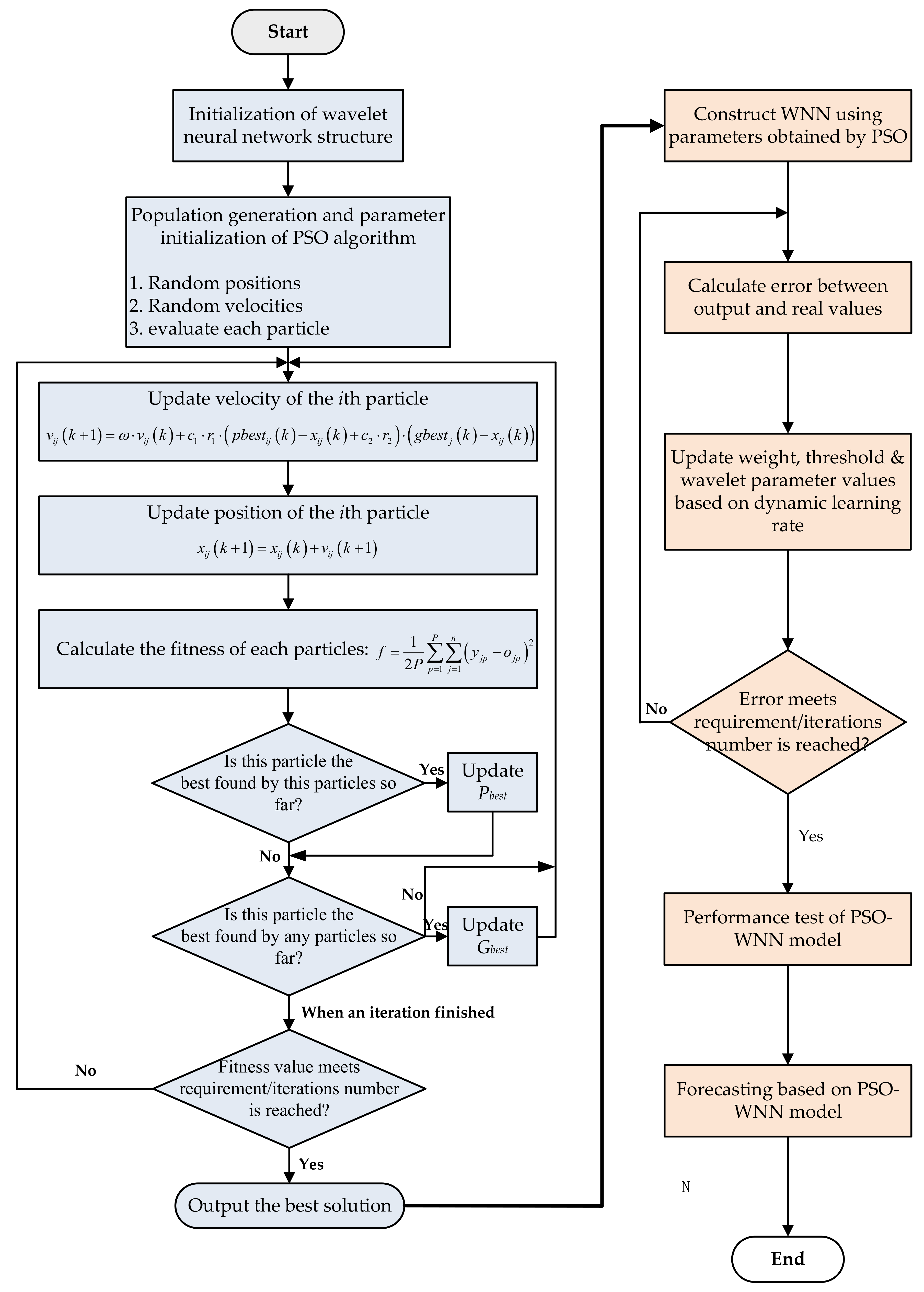
3. Hybrid PSO-WNN Forecasting model
- Step 1: Initialization. Initialize the neural network structures including the number of layers, the number of nodes in each layer, the weight values of WNN, and , and the parameters of wavelet, and . Initialize the parameters of PSO algorithm including the two positive constants and , the maximum particle velocity, and the total number of particles denoted by .
- Step 2: Population generation. Code the four neural network parameters including and as the particle position vector, i.e.,where represents the position of the ith particle. Then, randomly generate a number of particles as an initial population denoted by using both random and artificial ways. The position of each particle represents one feasible solution.
- Step 3: Fitness calculation. Calculate the difference between network’s output and real values and take this difference as the fitness function of PSO algorithm, i.e.,then, calculate the fitness of each particle according to Equation (7), and take the smallest fitness value as the initial values of Pbest and Gbest.
- Step 4: Update the Pbest. Compare the fitness of each particle () with Pbest. If , then replace Pbest by , i.e., .
- Step 5: Update the Gbest. Compare the fitness of each particle () with Gbest. If , then replace Gbest by , i.e., .
- Step 6: Update the position and velocity vectors of particles using the Equations (1) and (2).
- Step 7: Stop the PSO algorithm if one of the following is reached: (1) the current iteration number has reached the maximum number of generations; or (2) the fitness value of the particles remains constant for 50 iterations. Then, output the best particle which includes the best combination of and , and go to Steps 8–10 for training the WNN using the training sample. Otherwise, return to Step 3.
- Step 8: Calculate the output vector. Input the sample, obtain the output of the hidden neuron through the following Equation (8).where is the Morlet wavelet function, . For the sample, calculate the output of the neuron in the output layer through the following way:where is the threshold value of the neuron in the output layer.
- Step 9: Update and according to Equations (10)–(13).
- Step 10: Train the network until a set of and that satisfies , where is the pre-specified error and is the real value vector related to input sample , is found.
- Step 1: In the training process of the network, if the total error denoted by of iteration is larger than that of iteration, and the difference between them is larger than the pre-specified value (specified as 3% in this study), then this updating process is ignored and modify the learning rate by .
- Step 2: If , then update and . Modify the learning rate by .
- Step 3: If , while the increasing rate is less than , update and and keep the current learning rate value.
- Step 4: The above process of updating the learning rate can be summarized as follows.
4. Performance Test of the Hybrid PSO-WNN Forecasting Model
4.1. Affecting Factors of Natural Gas Consumption in China
- Economic growth. Previous studies show that China’s economic growth is the Granger cause of energy consumption growth. Energy demand and consumption tends to grow in line with GDP, although typically at a lower rate. Natural gas, which not only plays the role of important energy in the social development, but also an important raw chemical material in the industrial production, is the important original force of the economic development. Therefore, economic growth reflects the consumption of natural gas. However, due to the huge population of China, the GDP may not be related to an individual’s income. Thus, in this study, per capita GDP is used to measure the economic growth.
- Total amount of gas production (TP). The energy production has close relation with consumption. Natural gas, which is a non-renewable resource, should be produced according to the demand. Therefore, natural gas production has a positive or negative effect on consumption. In recent years, the increasing proportion of natural gas in the energy production structure promotes the growth of consumption.
- Household consumption level (HCL). With increasing of household consumption level, the public environmental awareness and quality of life improve greatly, which promote the wide use of natural gas in China.
- Population with access to gas (PAG). The population with access to gas is an important index to reflect the number of gas users. The population with access to gas increases with the development of gas infrastructure, which will drive more gas consumption.
- Urbanization ratio (UR). Urban and rural residents behave differently in terms of gas use and consumption level. Urban residents have access to better gas services because of better gas supply infrastructure such as urban gas pipelines. It is obviously that urban population growth stimulates the gas consumption. However, rural residents are less privileged in this aspect since they could not afford commercial gas consumption due to their income level. At current stage, China’s rural residents contribute little to the total gas consumption. Therefore, urbanization ratio is considered as an important gas consumption factor.
- Gas price (GP). According to accepted economic theory, price is the primary factor that affects consumption and the important lever for the balance of supply and demand. Price has a significant effect on consumer behavior. When the gas price is too high, users will use some other energy sources such as electricity or coal. In China, even though the gas pricing mechanisms has been changed from the previous cost-plus pricing method to the net market value pricing method, the current gas pricing process is still regulated by the government, and thus cannot fully reflect the scarcity of natural gas [26]. Therefore, the gas price is not considered as an affecting factor in this study.
4.2. Correlation Analysis between the Affecting Factors and Natural Gas Consumption
4.3. Models Comparison
5. Scenario Analysis of Natural Gas Consumption in China during 2017–2025
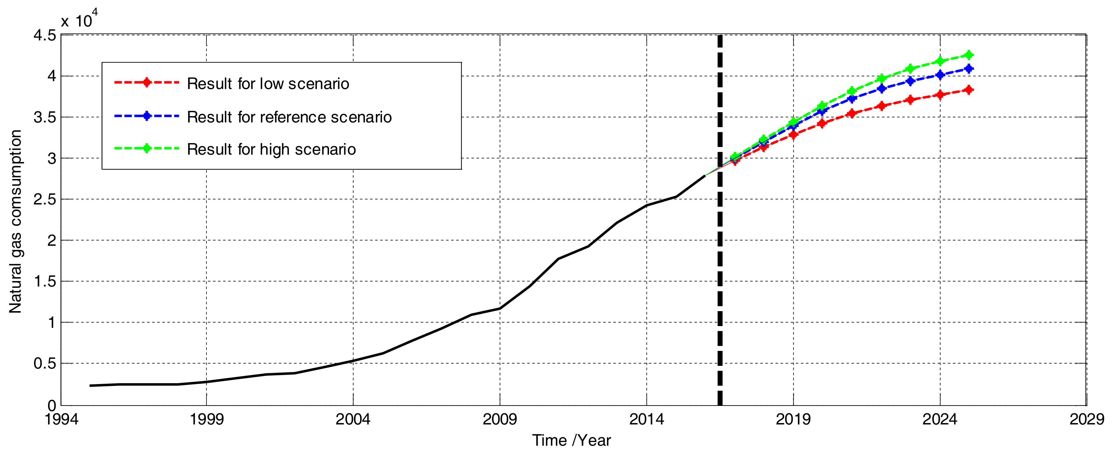
- Based on the results of scenario analysis, the China’s natural gas consumption is going to be 342.70, 358.27, 366.42 million tce (“standard” tons coal equivalent) in 2020, and 407.01, 437.95, 461.38 million tce in 2025 under the low, reference and high scenarios, respectively.
- The natural gas consumption in the high, reference and low scenarios have a similar increasing trend, while, over time, the gap of natural gas consumption between high and low cases becomes larger and larger.
- In all three scenarios, natural gas consumption increases relatively rapid from 2017 to 2020, while, after 2020, it increases relatively slow and has the trend to be relatively stable after 2025, which may be interpreted as, in the first four years (2017–2020), the five affecting factors have direct and important influences on the natural gas consumption, while, afterwards, many other factors such as policy and international energy environment, which are not considered in this study, will have influences on the forecasting results.
6. Conclusions
- The combination of five affecting factors, namely per capita GDP, total amount of gas production, household consumption level, population with access to gas and urbanization ratio, obtained using the correlation analysis, has significant or strong predictive ability for natural gas consumption in China.
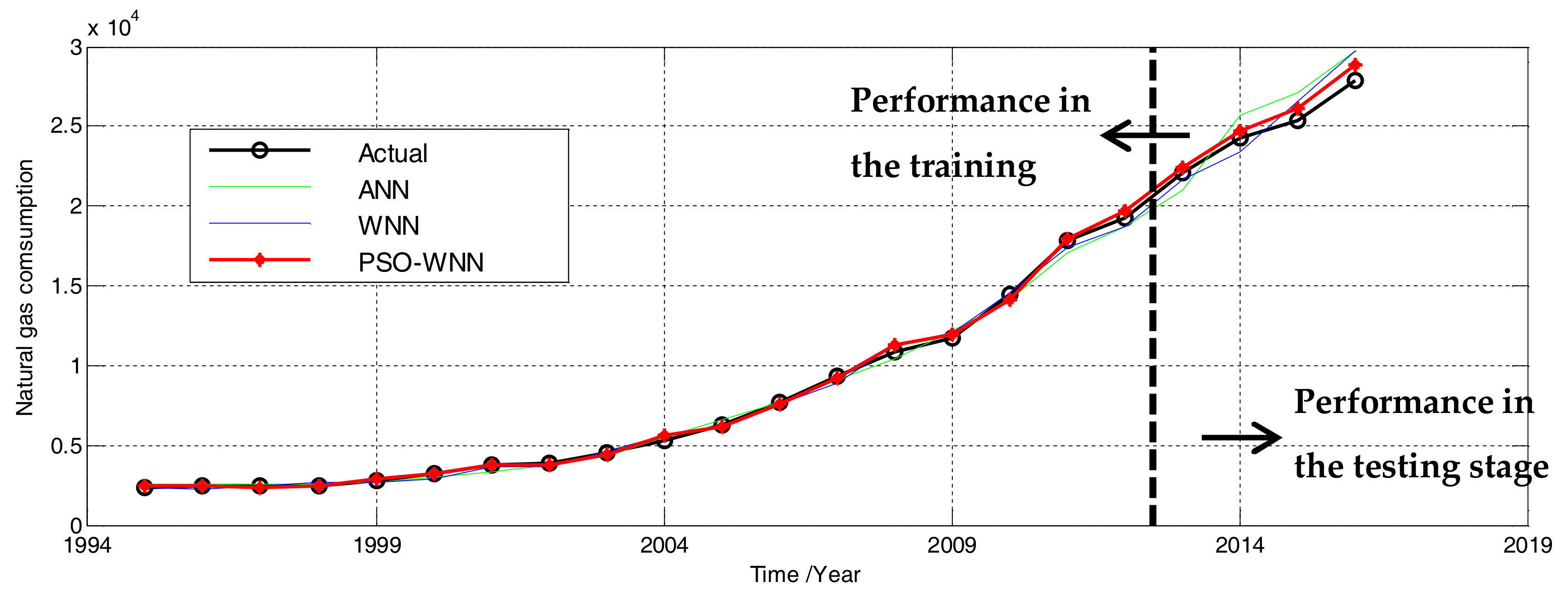
- The PSO-WNN model successfully predicts gas consumption as reflected by a MAPE value of 2.32% for prediction, and outperforms others. Based on the experiment shown in Figure 4, it is obviously that WNN model performs better than ANN model, which can be explained as, by combining the wavelet and neural work, WNN obtains strong function approximation ability, especially on the catastrophe points. Moreover, by adjusting the wavelet parameters and applying a dynamic learning rate mechanism for updating the connection weight values, WNN can effectively avoid falling into the local optimum. PSO-WNN model outperforms WNN model, which can be interpreted as the optimization of network weights and wavelet parameters using PSO algorithm effectively improves the forecasting precision and reduces fluctuation of WNN model.
- Natural gas consumption in China will keep a relatively rapid growing tendency. According to the results of scenario analysis, the China’s natural gas consumption is going to be 342.70, 358.27, 366.42 million tce (“standard” tons coal equivalent) in 2020, and 407.01, 437.95, 461.38 million tce in 2025 under the low, reference and high scenarios, respectively. To satisfy the increasing demand of natural gas consumption, the Chinese government should take some constructive measures: (a) The Chinese government should promote new exploration and development of natural gas reserves, especially in the southwest and northwest regions of China. The current estimation of natural gas resources indicates a URR of 22 trillion cubic meters, mainly distributed in southwest and northwest China; (b) The Chinese government should promote infrastructure construction such as enlargement of natural gas pipeline networks; (c) The Chinese government should accept that natural gas imports are unavoidable in future, thus seeking new suppliers and forging new relationships and collaborations in the gas sector are essential.
Acknowledgments
Author Contributions
Conflicts of Interest
Abbreviations
| ANN | Artificial neural network |
| ENN | Elman neural network |
| WNN | Wavelet neural network |
| PSO | Particle swarm optimization |
| PSO-WNN | Wavelet neural network optimized by particle swarm optimization algorithm |
| ARIMA | Auto-regressive integrated moving average |
| ARMA | Auto-regressive moving average |
| GM | Grey forecasting model |
| GARCH | Generalized autoregressive conditional heteroscedasticity |
| ELM | Extreme learning machine |
| SVM | Support vector machine |
| LSSVM | Least squares support vector machine |
| FAHP | Fuzzy C-Means integrating analytic hierarchy process |
| BP | Back propagation |
| GA | Genetic algorithm |
| GDP | Gross domestic product |
| TP | Total amount of gas production |
| HCL | Household consumption level |
| PAG | Population with access to gas |
| UR | Urbanization ratio |
| LP | Length of Pipeline |
| GP | Gas price |
| MAPE | Mean absolute percentage error |
References
- International Energy Agency (IEA). World Energy Outlook; Head of Communication and Information Office: Paris, France, 2010. Available online: http://www.iea.org/ (accessed on 15 October 2017).
- Shaikh, F.; Ji, Q. Forecasting natural gas demand in China: Logistic modelling analysis. Electr. Power Energy Syst. 2016, 77, 25–32. [Google Scholar] [CrossRef]
- Xu, W.J.; Gu, R.; Liu, Y.Z.; Dai, Y.W. Forecasting energy consumption using a new GM-ARMA model based on HP filter: The case of Guangdong province of China. Econ. Model. 2015, 45, 127–135. [Google Scholar] [CrossRef]
- Sen, P.; Roy, M.; Pal, P. Application of ARIMA for forecasting energy consumption and GHG emission: A case study of an Indian pig iron manufacturing organization. Energy 2016, 116, 1031–1038. [Google Scholar] [CrossRef]
- Zeng, B.; Li, C. Forecasting the natural gas demand in China using a self-adapting intelligent grey model. Energy 2016, 112, 810–825. [Google Scholar] [CrossRef]
- Wang, Y.D.; Wu, C.F. Forecasting energy market volatility using GARCH models: Can multivariate models beat univariate models? Energy Econ. 2012, 34, 2167–2181. [Google Scholar] [CrossRef]
- Wang, D.Y.; Luo, H.Y.; Grunder, O.; Lin, Y.B.; Guo, H.X. Multi-step ahead electricity price forecasting using a hybrid model based on two-layer decomposition technique and BP neural network optimized by firefly algorithm. Appl. Energy 2017, 190, 390–407. [Google Scholar] [CrossRef]
- Geng, Z.Q.; Qin, L.; Han, Y.M.; Zhu, Q.X. Energy saving and prediction modeling of petrochemical industries: A novel ELM based on FAHP. Energy 2017, 122, 350–362. [Google Scholar] [CrossRef]
- Ahmad, A.S.; Hassan, M.Y.; Abdullah, M.P.; Rahman, H.A.; Hussin, F.; Abdullah, H.; Saidur, R. A review on applications of ANN and SVM for building electrical energy consumption forecasting. Renew. Sustain. Energy Rev. 2014, 33, 102–109. [Google Scholar] [CrossRef]
- Barman, M.; Choudhury, N.B.D.; Sutradhar, S. A regional hybrid GOA-SVM model based on similar day approach for short-term load forecasting in Assam, India. Energy 2018, 145, 710–720. [Google Scholar] [CrossRef]
- Niu, D.; Dai, S. A short-term load forecasting model with a modified particle swarm optimization algorithm and least squares support vector machine based on the denoising method of empirical mode decomposition and grey relational analysis. Energies 2017, 10, 408. [Google Scholar] [CrossRef]
- Zhang, R.; Dong, Z.; Xu, Y.; Meng, K.; Wong, K. Short-term load forecasting of Australian national electricity market by an ensemble model of extreme learning machine. IET Gener. Transm. Distrib. 2013, 7, 391–397. [Google Scholar] [CrossRef]
- Chaturvedi, D.; Sinha, A.; Malik, O. Short term load forecast using fuzzy logic and wavelet transform integrated generalized neural network. Electr. Power Energy Syst. 2015, 67, 230–237. [Google Scholar] [CrossRef]
- Li, S.; Wang, P.; Goel, L. A novel wavelet-based ensemble method for short-term load forecasting with hybrid neural networks and feature selection. IEEE Trans. Power Syst. 2016, 31, 1788–1798. [Google Scholar] [CrossRef]
- Fard, A.K.; Akbari-Zadeh, M.R. A hybrid method based on wavelet, ANN and ARIMA model for short-term load forecasting. J. Exp. Theor. Artif. Intell. 2014, 26, 167–182. [Google Scholar] [CrossRef]
- Karimi, H.; Dastranj, J. Artificial neural network-based genetic algorithm to predict natural gas consumption. Energy Syst. 2014, 5, 571–581. [Google Scholar] [CrossRef]
- Muralitharan, K.; Sakthivel, R.; Vishnuvarthan, R. Neural network based optimization approach for energy demand prediction in smart grid. Neurocomputing 2018, 273, 199–208. [Google Scholar] [CrossRef]
- Ren, G.H.; Cao, Y.T.; Wen, S.P.; Huang, T.W.; Zeng, Z.G. A modified Elman neural network with a new learning rate scheme. Neurocomputing 2018, 286, 11–18. [Google Scholar] [CrossRef]
- Wang, S.X.; Zhang, N.; Wu, L.; Wang, Y.M. Wind speed forecasting based on the hybrid ensemble empirical mode decomposition and GA-BP neural network method. Renew. Energy 2016, 94, 629–636. [Google Scholar] [CrossRef]
- Wang, D.Y.; Liu, Y.L.; Luo, H.Y.; Yue, C.Q.; Cheng, S. Day-Ahead PM2.5 Concentration Forecasting Using WT-VMD Based Decomposition Method and Back Propagation Neural Network Improved by Differential Evolution. Int. J. Environ. Res. Public Health 2017, 14, 764. [Google Scholar] [CrossRef] [PubMed]
- Wang, D.Y.; Wei, S.; Luo, H.Y.; Yue, C.Q.; Grunder, O. A novel hybrid model for air quality index forecasting based on two-phase decomposition technique and modified extreme learning machine. Sci. Total Environ. 2017, 580, 719–733. [Google Scholar] [CrossRef] [PubMed]
- Del Valle, Y.; Venayagamoorthy, G.K.; Mohagheghi, S.; Hernandez, J.C.; Harley, R.G. Particle swarm optimization: Basic concepts, variants and applications in power systems. IEEE Trans. Evol. Comput. 2008, 12, 171–195. [Google Scholar] [CrossRef]
- Kucuk, M.; Agiralioglu, N. Wavelet regression techniques for stream flow predictions. J Appl. Stat. 2006, 33, 943–960. [Google Scholar] [CrossRef]
- Wang, D.Y.; Luo, H.Y.; Grunder, O.; Lin, Y.B. Multi-step ahead wind speed forecasting using an improved wavelet neural network combining variational mode decomposition and phase space reconstruction. Renew. Energy 2017, 113, 1345–1358. [Google Scholar] [CrossRef]
- Luo, D. K; Xu, P. Natural gas demand forecasting based on improved BP. Oil-Gas Ground Eng. 2008, 27, 20–21. [Google Scholar]
- Wang, F.; Liu, X. An economic analysis of natural gas price-forming mechanisms in China: From the previous cost-plus pricing method to the net market value pricing method. Nat. Gas Ind. 2014, 34, 135–142. [Google Scholar]
- Fang, S.S.; Yao, X.S.; Zhang, J.Q.; Han, M. Grey correlation analysis on travel modes and their influence factors. Procedia Eng. 2017, 174, 347–352. [Google Scholar] [CrossRef]
- Song, W.J.; Wang, L.Z.; Xiang, Y.; Zomaya, A.Y. Geographic spatiotemporal big data correlation analysis via the Hilbert-Huang transformation. J. Comput. Syst. Sci. 2017, 89, 130–141. [Google Scholar] [CrossRef]
- National Bureau of Statistics of PRC. Available online: http://www.stats.gov.cn/tjsj/ndsj/ (accessed on 12 March 2018).
- Bianco, V.; Scarpa, F.; Tagliafico, L.A. Scenario analysis of nonresidential natural gas consumption in Italy. Appl. Energy 2014, 113, 392–403. [Google Scholar] [CrossRef]
- Osicka, J.; Ocelik, P.; Dancak, B. The impact of Polish unconventional production on the regional distribution of natural gas supply and transit: A scenario analysis. Energy Strateg. Rev. 2016, 10, 1–17. [Google Scholar] [CrossRef]


| Absolute Value of Correlation | Correlation Level | Absolute Value of Correlation | Correlation Level |
|---|---|---|---|
| Linear | Significant | ||
| Strong | Moderate | ||
| Weak | Nonexistent |
| No. | Affecting Factors | Correlation Degree | Correlation Level | Sorting of Correlation Degree |
|---|---|---|---|---|
| 1 | GDP per capita (GDP) | 0.8396 | Strong | 5 |
| 2 | Total amount of gas production (TP) | 0.9834 | Significant | 1 |
| 3 | Household consumption level (HCL) | 0.9751 | Significant | 2 |
| 4 | Population with access to gas (PAG) | 0.9737 | Significant | 3 |
| 5 | Urbanization ratio (UR) | 0.8725 | Strong | 4 |
| 6 | length of Pipeline (LP) | 0.6971 | Moderate | 6 |
| Year | Per Capita GDP | TP | HCL | PAG | UR | NGC |
|---|---|---|---|---|---|---|
| 1995 | 5091 | 2451.65 | 2355 | 859.8 | 29.04 | 23.61 |
| 1996 | 5898 | 2660.64 | 2789 | 1470.0 | 30.48 | 24.33 |
| 1997 | 6481 | 2802.66 | 3002 | 1656.2 | 31.91 | 24.46 |
| 1998 | 6860 | 2856.35 | 3159 | 1908.1 | 33.35 | 24.51 |
| 1999 | 7229 | 3298.38 | 3346 | 2225.1 | 34.78 | 28.11 |
| 2000 | 7942 | 3646.30 | 3721 | 2581.0 | 36.22 | 32.33 |
| 2001 | 8717 | 4028.50 | 3987 | 3240.0 | 37.66 | 37.33 |
| 2002 | 9506 | 4369.02 | 4301 | 3686.0 | 39.09 | 39.00 |
| 2003 | 10,666 | 4641.46 | 4606 | 4320.2 | 40.53 | 45.33 |
| 2004 | 12,487 | 5506.14 | 5138 | 5627.6 | 41.76 | 52.96 |
| 2005 | 14,368 | 6486.57 | 5771 | 7104.4 | 42.99 | 62.73 |
| 2006 | 16,738 | 7893.68 | 6416 | 8319.4 | 44.34 | 77.35 |
| 2007 | 20,505 | 9149.32 | 7572 | 10,189.8 | 45.89 | 93.43 |
| 2008 | 24,121 | 10,656.58 | 8707 | 12,167.1 | 46.99 | 109.01 |
| 2009 | 26,222 | 11,259.38 | 9514 | 14,543.7 | 48.34 | 117.64 |
| 2010 | 30,876 | 12,470.47 | 10,919 | 17,021.2 | 49.95 | 144.26 |
| 2011 | 36,403 | 13,673.44 | 13,134 | 19,027.8 | 51.27 | 178.04 |
| 2012 | 40,007 | 14,269.46 | 14,699 | 21,207.5 | 52.57 | 193.02 |
| 2013 | 43,852 | 15,640.00 | 16,190 | 23,783.4 | 53.73 | 220.96 |
| 2014 | 47,203 | 17,007.70 | 17,778 | 25,972.94 | 54.77 | 242.70 |
| 2015 | 50,251 | 17,350.85 | 19,397 | 28,561.47 | 56.10 | 253.64 |
| 2016 | 53,980 | 18,338.00 | 21,228 | 30,855.57 | 57.35 | 279.04 |
| Year | Actual | ANN Fittings | |Error| (%) | WNN Fittings | |Error| (%) | PSO-WNN Fittings | |Error| (%) |
|---|---|---|---|---|---|---|---|
| 1995 | 23.61 | 25.71 | 8.89 | 23.82 | 0.89 | 24.06 | 1.91 |
| 1996 | 24.33 | 25.65 | 5.43 | 22.52 | 7.44 | 24.11 | 0.90 |
| 1997 | 24.46 | 25.87 | 5.76 | 25.03 | 2.33 | 23.89 | 2.33 |
| 1998 | 24.51 | 25.76 | 5.10 | 26.19 | 6.85 | 24.82 | 1.26 |
| 1999 | 28.11 | 26.87 | 4.41 | 27.21 | 3.20 | 28.55 | 1.57 |
| 2000 | 32.33 | 30.22 | 6.53 | 29.28 | 9.43 | 32.68 | 1.08 |
| 2001 | 37.33 | 32.94 | 11.76 | 36.41 | 2.46 | 37.92 | 1.58 |
| 2002 | 39.00 | 37.82 | 3.03 | 36.71 | 5.87 | 38.12 | 2.26 |
| 2003 | 45.33 | 43.07 | 4.99 | 46.26 | 2.05 | 44.29 | 2.29 |
| 2004 | 52.96 | 54.70 | 3.29 | 55.86 | 5.48 | 55.99 | 5.72 |
| 2005 | 62.73 | 66.02 | 5.24 | 61.37 | 2.17 | 61.75 | 1.56 |
| 2006 | 77.35 | 76.83 | 0.67 | 75.69 | 2.15 | 76.28 | 1.38 |
| 2007 | 93.43 | 91.10 | 2.49 | 89.25 | 4.47 | 92.28 | 1.23 |
| 2008 | 109.01 | 103.90 | 4.69 | 112.88 | 3.55 | 112.71 | 3.39 |
| 2009 | 117.64 | 122.17 | 3.85 | 120.78 | 2.67 | 119.12 | 1.26 |
| 2010 | 144.26 | 140.87 | 2.35 | 145.61 | 0.94 | 141.60 | 1.84 |
| 2011 | 178.04 | 170.27 | 4.36 | 173.86 | 2.35 | 179.81 | 0.99 |
| 2012 | 193.02 | 187.46 | 2.88 | 187.32 | 2.95 | 197.13 | 2.13 |
| MAPE | - | - | 4.76 | - | 3.74 | - | 1.93 |
| Year | Actual | Forecast Value of ANN | |Error| (%) | Forecast Value of WNN | |Error| (%) | Forecast Value of PSO-WNN | |Error| (%) |
| 2013 | 220.96 | 209.71 | 5.09 | 216.59 | 1.98 | 223.70 | 1.24 |
| 2014 | 242.70 | 256.60 | 5.73 | 234.43 | 3.41 | 247.14 | 1.83 |
| 2015 | 253.64 | 270.85 | 6.79 | 265.42 | 4.64 | 261.09 | 2.94 |
| 2016 | 279.04 | 297.22 | 6.52 | 297.07 | 6.46 | 288.11 | 3.25 |
| MAPE | - | - | 6.03 | - | 4.12 | - | 2.31 |
| Scenarios Settings | Per Capital GDP | TP | HCL | PAG | UR |
|---|---|---|---|---|---|
| Increasing rate in low scenario | 6.0% | 5.0% | 12.0% | 9.0% | 1.5% |
| Increasing rate in reference scenario | 7.0% | 6.0% | 14.0% | 11.0% | 2.0% |
| Increasing rate in high scenario | 8.0% | 7.0% | 16.0% | 13.0% | 2.5% |
| Year | Per Capital GDP | TP | HCL | PAG | UR (%) | NGC | |
|---|---|---|---|---|---|---|---|
| Low-scenario | 2017 | 57,218.80 | 19,254.90 | 23,775.36 | 33,632.57 | 58.21 | 297.18 |
| 2018 | 60,651.93 | 20,217.65 | 26,628.40 | 36,659.50 | 59.08 | 313.52 | |
| 2019 | 64,291.04 | 21,228.53 | 29,823.81 | 39,958.86 | 59.97 | 328.89 | |
| 2020 | 68,148.51 | 22,289.95 | 33,402.67 | 43,555.16 | 60.87 | 342.70 | |
| 2021 | 72,237.42 | 23,404.45 | 37,410.99 | 47,475.12 | 61.78 | 356.06 | |
| 2022 | 76,571.66 | 24,574.67 | 41,900.31 | 51,747.88 | 62.71 | 369.24 | |
| 2023 | 81,165.96 | 25,803.41 | 46,928.34 | 56,405.19 | 63.65 | 382.53 | |
| 2024 | 86,035.92 | 27,093.58 | 52,559.75 | 61,481.66 | 64.60 | 395.15 | |
| 2025 | 91,198.07 | 28,448.26 | 58,866.92 | 67,015.01 | 65.57 | 407.01 | |
| Refer-scenario | 2017 | 57,758.60 | 19,438.28 | 24,199.92 | 34,249.68 | 58.50 | 299.97 |
| 2018 | 61,801.70 | 20,604.58 | 27,587.91 | 38,017.15 | 59.67 | 319.77 | |
| 2019 | 66,127.82 | 21,840.85 | 31,450.22 | 42,199.03 | 60.86 | 339.59 | |
| 2020 | 70,756.77 | 23,151.30 | 35,853.25 | 46,840.93 | 62.08 | 358.27 | |
| 2021 | 75,709.74 | 24,540.38 | 40,872.70 | 51,993.43 | 63.32 | 376.18 | |
| 2022 | 81,009.42 | 26,012.80 | 46,594.88 | 57,712.71 | 64.59 | 393.11 | |
| 2023 | 86,680.08 | 27,573.57 | 53,118.16 | 64,061.10 | 65.88 | 408.84 | |
| 2024 | 92,747.69 | 29,227.99 | 60,554.70 | 71,107.83 | 67.19 | 423.96 | |
| 2025 | 99,240.03 | 30,981.67 | 69,032.36 | 78,929.69 | 68.54 | 437.95 | |
| High-scenario | 2017 | 58,298.40 | 19,621.66 | 24,624.48 | 34,866.79 | 58.78 | 301.36 |
| 2018 | 62,962.27 | 20,995.18 | 28,564.40 | 39,399.48 | 60.25 | 323.06 | |
| 2019 | 67,999.25 | 22,464.84 | 33,134.70 | 44,521.41 | 61.76 | 345.03 | |
| 2020 | 73,439.19 | 24,037.38 | 38,436.25 | 50,309.19 | 63.30 | 366.42 | |
| 2021 | 79,314.33 | 25,719.99 | 44,586.05 | 56,849.39 | 64.89 | 387.67 | |
| 2022 | 85,659.48 | 27,520.39 | 51,719.82 | 64,239.81 | 66.51 | 409.00 | |
| 2023 | 92,512.23 | 29,446.82 | 59,994.99 | 72,590.98 | 68.17 | 428.22 | |
| 2024 | 99,913.21 | 31,508.10 | 69,594.19 | 82,027.81 | 69.88 | 445.78 | |
| 2025 | 107,906.27 | 33,713.67 | 80,729.26 | 92,691.43 | 71.62 | 461.38 |
© 2018 by the authors. Licensee MDPI, Basel, Switzerland. This article is an open access article distributed under the terms and conditions of the Creative Commons Attribution (CC BY) license (http://creativecommons.org/licenses/by/4.0/).
Share and Cite
Wang, D.; Liu, Y.; Wu, Z.; Fu, H.; Shi, Y.; Guo, H. Scenario Analysis of Natural Gas Consumption in China Based on Wavelet Neural Network Optimized by Particle Swarm Optimization Algorithm. Energies 2018, 11, 825. https://doi.org/10.3390/en11040825
Wang D, Liu Y, Wu Z, Fu H, Shi Y, Guo H. Scenario Analysis of Natural Gas Consumption in China Based on Wavelet Neural Network Optimized by Particle Swarm Optimization Algorithm. Energies. 2018; 11(4):825. https://doi.org/10.3390/en11040825
Chicago/Turabian StyleWang, Deyun, Yanling Liu, Zeng Wu, Hongxue Fu, Yong Shi, and Haixiang Guo. 2018. "Scenario Analysis of Natural Gas Consumption in China Based on Wavelet Neural Network Optimized by Particle Swarm Optimization Algorithm" Energies 11, no. 4: 825. https://doi.org/10.3390/en11040825
APA StyleWang, D., Liu, Y., Wu, Z., Fu, H., Shi, Y., & Guo, H. (2018). Scenario Analysis of Natural Gas Consumption in China Based on Wavelet Neural Network Optimized by Particle Swarm Optimization Algorithm. Energies, 11(4), 825. https://doi.org/10.3390/en11040825