Performance Analysis of Short-Term Electricity Demand with Atmospheric Variables
Abstract
1. Introduction
2. Description of Data
2.1. Electricity Demand Data
2.2. Atmospheric Variables
2.3. Weather Station Selection
3. Related Works
4. Prototype Modeling
4.1. Modeling Trend
4.2. Modeling Cyclicality and Seasonality
4.3. Mathematical Model
- Model A: This model consists of the variables from deterministic terms, historical demand and historical demand-related interaction (e.g., ) term. Therefore, Model A is the sum of Equations (5), (9) and (10) and consists of a total of 47 variables including six correlated error terms (). The electricity demand from Model A is denoted by and can be generalized as,
- Model C: Model C consists of all the variables from Model B and atmospheric variables (Equation (8)). Therefore, Model C consists of 94 variables. The electricity demand from Model C is represented by and can be generalized as,
5. Estimation and Forecasting
Algorithm Setup
- Set informative priors,
- Starting values, . The suffix ‘’ in the symbol means OLS estimation.
- Set a normal prior for serial correlated coefficient as , with starting value .
- Set an inverse Gamma prior for where and represent the degree of freedom and scale factor, respectively.
- Draw the conditional posterior distribution,
- For , , then (Appendix C, Theorem A1)
- For correlated error , , then (Appendix C, Theorem A1)
- Given a draw from and , draw from its conditional posterior distribution, . (Appendix C, Theorem A2)
- Repeat Steps 2 and 3 M times to obtain and .
6. Results and Discussion
6.1. Atmospheric Variables
6.2. Temperature Variables
6.3. Performance Analysis
6.4. Hypothesis Testing
6.5. Computation Time
7. Conclusions
Acknowledgments
Author Contributions
Conflicts of Interest
Abbreviations
| ARMAX | Auto-regressive moving average with exogenous variable |
| MAPE | Mean absolute percentage error |
| IPCC | Intergovernmental Panel on Climate Change |
| MLR | Multiple linear regression |
| ANN | Artificial neural network |
| SVM | Support vector machine |
| GEFCom2012 | Global Energy Forecasting Competition 2012 |
| CDD | Cooling degree day |
| HDD | Heating degree day |
| HEPCO | Hokkaido Electrical Power Company |
| JMA | Japan Meteorological Agency |
| MW | Megawatt |
| OLS | Ordinary least square |
| MCMC | Markov chain Monte Carlo |
Appendix A. Weather Station Selection
Appendix A.1. Methodology
Appendix A.2. Algorithm Setup
- Denote the temperature variables (daily average, maximum and minimum temperature) of each stations as , .
- Develop the forecasting model (Equation (A1)) where electricity demand is a function of the temperature and calendar variables.
- For speed and simplicity, use OLS estimation and forecasting for a year out of the sample data.
- Calculate the forecasting error and MAPE for all the weather stations separately.
- Sort the resulting error measures in ascending order to find the best individual’s (weather stations) impact on demand.
- Combine (average and weighted average with population) the temperature data of the top k weather stations to create a new temperature series and fit all these combinations to the same forecasting model.
- Calculate the forecasting error and find the combinations of weather stations that give the best (smallest) MAPE.
| Weather Station | Forecasting Results of Weather Stations When Their Data Combined as: | |||||||||||
|---|---|---|---|---|---|---|---|---|---|---|---|---|
| Simple Mean | Weighted by Population | |||||||||||
| Sub-Prefecture | Area (m2) | Population | Name | Index | MAPE (%) | Combination | MAPE (%) Variance | R2 | Adjusted-R2 | MAPE (%) Variance | R2 | Adjusted-R2 |
| Ishikari | 3539.86 | 2,324,878 | Sapporo | 1 | 2.959 | 1, and 2 | 3.012(1.702) | 0.943 | 0.938 | 2.945(1.70) | 0.965 | 0.962 |
| Kamikawa | 10,619.20 | 527,575 | Hakodate | 2 | 3.042 | 1, 2 and 7 | 2.894(1.667) | 0.946 | 0.941 | 2.909(1.689) | 0.968 | 0.965 |
| Oshima | 3936.46 | 433,475 | Kitami | 3 | 3.318 | 1, 2, 7 and 8 | 2.967(1.841) | 0.943 | 0.938 | 2.942(1.744) | 0.966 | 0.963 |
| Iburi | 3698 | 419,115 | Abashiri | 4 | 3.323 | 1, 2, 7, 8 and 6 | 3.324(1.909) | 0.930 | 0.924 | 3.324(1.90) | 0.962 | 0.959 |
| Ashahikawa | 5 | 3.174 | 1, 2, 7, 8, 6 and 5 | 2.970(1.792) | 0.943 | 0.937 | 2.946(1.725) | 0.965 | 0.962 | |||
| Tokachi | 10,831.24 | 353,291 | Obihiro | 6 | 3.169 | 1, 2, 7, 8, 6, 5 and 3 | 2.899(1.730) | 0.945 | 0.940 | 2.905(1.710) | 0.967 | 0.964 |
| Okhotsk | 10,690.62 | 309487 | Moruran | 7 | 3.010 | 1, 2, 7, 8, 6, 5, 3 and 4 | 2.925(1.670) | 0.945 | 0.940 | 2.927(1.675) | 0.968 | 0.965 |
| Tomakomai | 8 | 3.156 | ||||||||||
Appendix B. Forecasting Example
Appendix C. Theorems
Appendix C.1. Theorem A1
Appendix C.2. Theorem A2
Appendix D. Figures and Tables
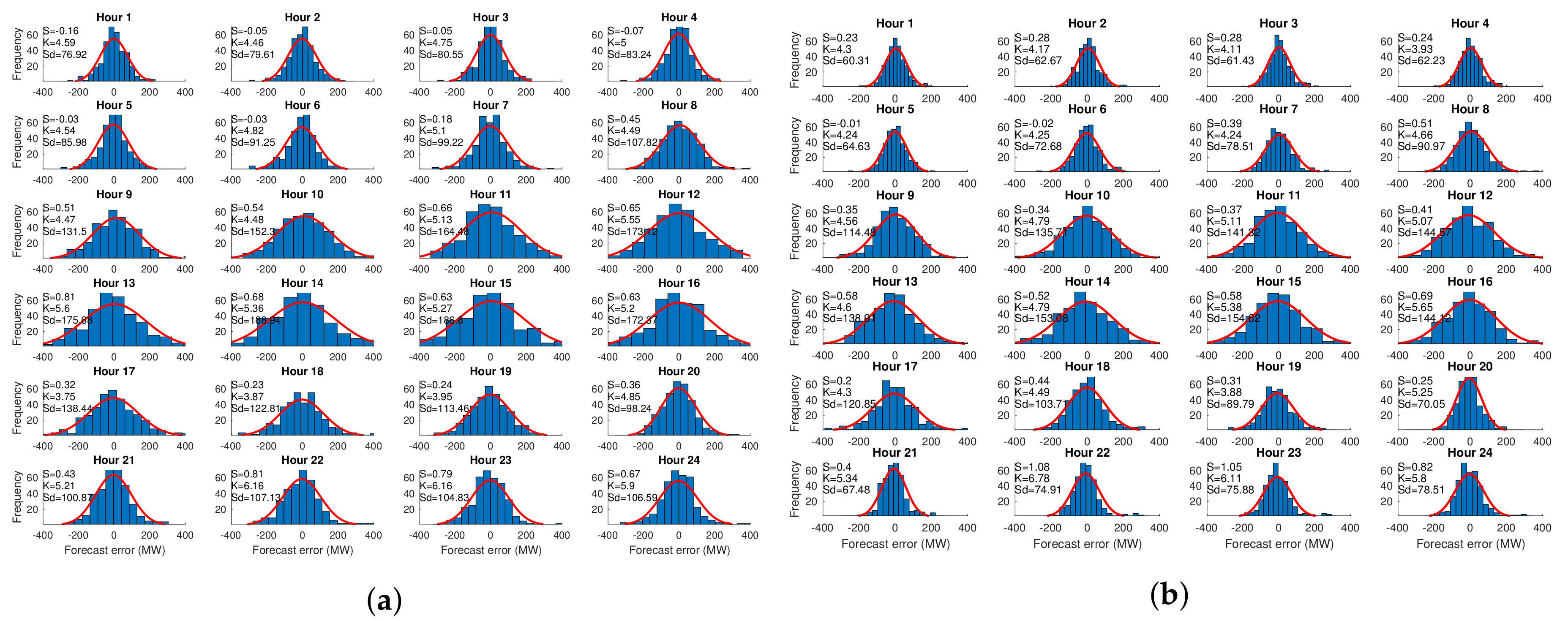
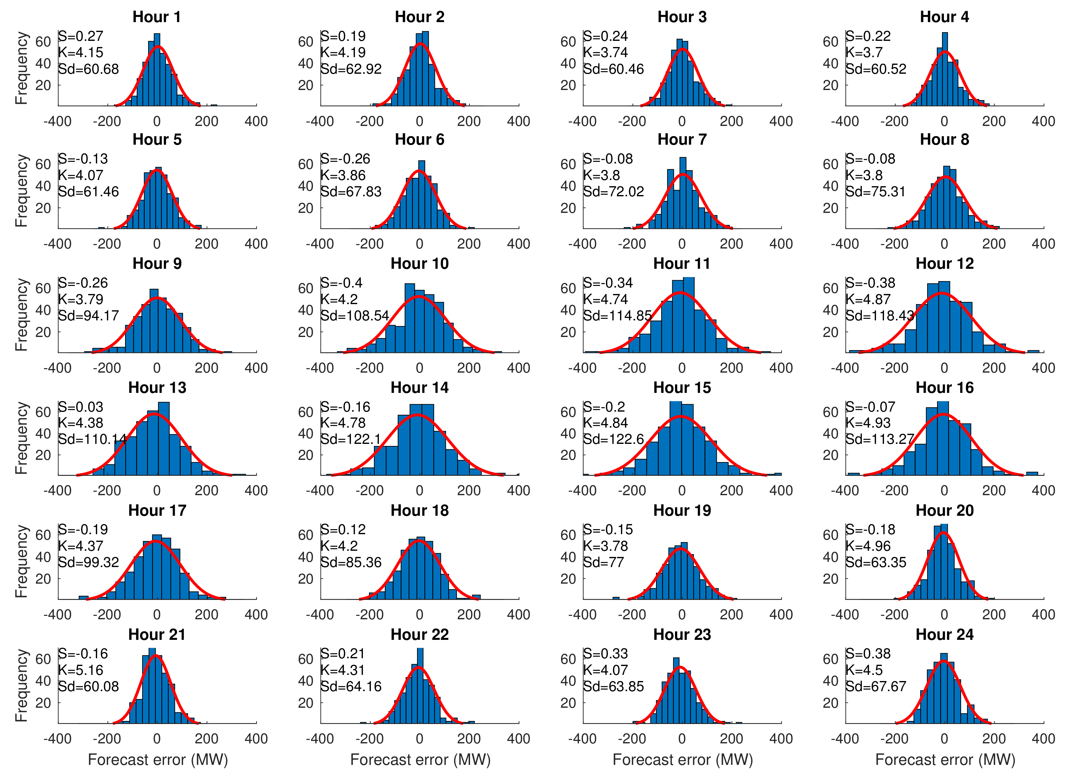
| Hour | Model | Sunday | Monday | Tuesday | Wednesday | Thursday | Friday | Saturday | WDH | WDNH | WEH | WENH | HWD | HWE | Holiday | NH |
|---|---|---|---|---|---|---|---|---|---|---|---|---|---|---|---|---|
| 1 | Model A | 1.6726 | 1.7407 | 1.7456 | 1.8309 | 1.5394 | 1.4631 | 1.4922 | 1.6639 | 0.7753 | 1.5824 | 1.6213 | 1.9812 | 0.8121 | 1.7474 | 1.6325 |
| Model B | 1.1504 | 1.4382 | 1.2741 | 1.4257 | 1.2117 | 1.4709 | 1.2896 | 1.3642 | 0.7606 | 1.2200 | 1.2131 | 1.4685 | 1.3576 | 1.4463 | 1.3136 | |
| Model C | 1.1919 | 1.4357 | 1.3395 | 1.4745 | 1.1992 | 1.5799 | 1.2373 | 1.4057 | 0.8193 | 1.1919 | 1.2274 | 1.6611 | 0.9614 | 1.5212 | 1.3382 | |
| 2 | Model A | 1.8561 | 1.7041 | 1.6715 | 1.8159 | 1.5774 | 1.5581 | 1.5430 | 1.6654 | 0.8006 | 1.6996 | 1.7156 | 2.1112 | 1.3818 | 1.9653 | 1.6535 |
| Model B | 1.2177 | 1.4480 | 1.1882 | 1.4230 | 1.2913 | 1.5818 | 1.4109 | 1.3865 | 0.7887 | 1.3143 | 1.3056 | 1.3492 | 1.4865 | 1.3767 | 1.3648 | |
| Model C | 1.2970 | 1.4602 | 1.1697 | 1.4413 | 1.2717 | 1.6941 | 1.3749 | 1.4074 | 0.8426 | 1.2970 | 1.3407 | 1.5256 | 1.2430 | 1.4691 | 1.3806 | |
| 3 | Model A | 1.8299 | 1.6551 | 1.7280 | 1.8782 | 1.5712 | 1.3902 | 1.3610 | 1.6445 | 0.6908 | 1.5954 | 1.6039 | 2.2782 | 1.4283 | 2.1082 | 1.5952 |
| Model B | 1.2882 | 1.3785 | 1.1462 | 1.4060 | 1.1784 | 1.3799 | 1.3110 | 1.2978 | 0.7097 | 1.2996 | 1.3006 | 1.2319 | 1.2804 | 1.2416 | 1.3021 | |
| Model C | 1.3373 | 1.3129 | 1.1836 | 1.3597 | 1.1587 | 1.4631 | 1.3420 | 1.2956 | 0.7436 | 1.3373 | 1.3548 | 1.3017 | 1.0399 | 1.2494 | 1.3121 | |
| 4 | Model A | 1.7652 | 1.6379 | 1.8458 | 1.8160 | 1.6098 | 1.3923 | 1.3475 | 1.6604 | 0.6981 | 1.5563 | 1.5657 | 2.2030 | 1.3701 | 2.0364 | 1.6007 |
| Model B | 1.1658 | 1.2604 | 1.1607 | 1.3288 | 1.2750 | 1.4508 | 1.3543 | 1.2952 | 0.7567 | 1.2600 | 1.2595 | 1.1060 | 1.2704 | 1.1389 | 1.2958 | |
| Model C | 1.1385 | 1.2825 | 1.1582 | 1.3299 | 1.1545 | 1.4228 | 1.3618 | 1.2696 | 0.7364 | 1.1385 | 1.2624 | 1.0859 | 1.0082 | 1.0704 | 1.2779 | |
| 5 | Model A | 1.8329 | 1.6645 | 1.9004 | 1.9173 | 1.5649 | 1.5715 | 1.3441 | 1.7237 | 0.7901 | 1.5885 | 1.5814 | 2.3748 | 1.7288 | 2.2456 | 1.6435 |
| Model B | 1.3387 | 1.3066 | 1.3126 | 1.3861 | 1.2598 | 1.4386 | 1.3605 | 1.3407 | 0.7509 | 1.3496 | 1.3297 | 1.4274 | 1.7425 | 1.4904 | 1.3322 | |
| Model C | 1.3420 | 1.3241 | 1.2364 | 1.4013 | 1.1265 | 1.4575 | 1.2308 | 1.3092 | 0.7773 | 1.3420 | 1.2897 | 1.3027 | 1.2207 | 1.2863 | 1.3033 | |
| 6 | Model A | 1.9198 | 1.9072 | 2.0596 | 1.9769 | 1.5467 | 1.5389 | 1.6301 | 1.8059 | 0.7545 | 1.7750 | 1.8003 | 2.5605 | 1.2725 | 2.3029 | 1.7591 |
| Model B | 1.6503 | 1.5450 | 1.6708 | 1.5754 | 1.1965 | 1.4065 | 1.5892 | 1.4789 | 0.7142 | 1.6197 | 1.5820 | 1.6762 | 2.3669 | 1.8144 | 1.4965 | |
| Model C | 1.6451 | 1.5607 | 1.5380 | 1.5917 | 1.1067 | 1.3907 | 1.4814 | 1.4376 | 0.7524 | 1.6451 | 1.5595 | 1.4951 | 1.6376 | 1.5236 | 1.4687 | |
| 7 | Model A | 2.0690 | 2.1267 | 2.2502 | 2.2338 | 1.8833 | 1.6164 | 1.9340 | 2.0221 | 0.7776 | 2.0015 | 2.0574 | 2.9955 | 0.8951 | 2.5754 | 1.9747 |
| Model B | 1.7640 | 1.7209 | 1.7645 | 1.6313 | 1.4183 | 1.4893 | 2.0553 | 1.6049 | 0.7315 | 1.9097 | 1.9323 | 2.4035 | 1.4605 | 2.2149 | 1.6527 | |
| Model C | 1.6466 | 1.7467 | 1.5595 | 1.5090 | 1.2270 | 1.4631 | 1.7972 | 1.5011 | 0.7673 | 1.6466 | 1.7573 | 2.0983 | 1.0206 | 1.8828 | 1.5397 | |
| 8 | Model A | 2.2325 | 2.3071 | 2.2233 | 2.5286 | 2.4832 | 2.1212 | 2.4363 | 2.3327 | 1.0441 | 2.3344 | 2.3803 | 3.4155 | 1.4263 | 3.0177 | 2.2833 |
| Model B | 1.8220 | 1.8314 | 1.9199 | 1.9725 | 1.8258 | 1.7969 | 2.5240 | 1.8693 | 0.8740 | 2.1730 | 2.1622 | 2.8535 | 2.3874 | 2.7603 | 1.8966 | |
| Model C | 1.5913 | 1.5995 | 1.5147 | 1.6427 | 1.4574 | 1.5827 | 2.1622 | 1.5594 | 0.8269 | 1.5913 | 1.8738 | 2.2654 | 1.9355 | 2.1994 | 1.6091 | |
| 9 | Model A | 2.6461 | 2.4470 | 2.7248 | 2.7950 | 2.8503 | 2.4008 | 3.1912 | 2.6436 | 1.1834 | 2.9187 | 2.8304 | 4.3900 | 4.6659 | 4.4452 | 2.5959 |
| Model B | 2.1982 | 2.0883 | 2.2785 | 2.2846 | 2.4666 | 2.1374 | 3.1797 | 2.2511 | 1.0574 | 2.6890 | 2.5874 | 3.8711 | 4.6995 | 4.0367 | 2.2544 | |
| Model C | 1.9150 | 1.7530 | 1.7447 | 1.9969 | 1.9034 | 1.8084 | 2.8321 | 1.8413 | 0.9390 | 1.9150 | 2.2789 | 3.4363 | 4.2477 | 3.5986 | 1.8751 | |
| 10 | Model A | 2.9442 | 2.6022 | 3.2205 | 3.0529 | 3.1272 | 2.6851 | 3.6793 | 2.9376 | 1.3814 | 3.3117 | 3.1540 | 4.5038 | 6.4350 | 4.8900 | 2.9090 |
| Model B | 2.4234 | 2.3307 | 2.6872 | 2.3936 | 2.7461 | 2.7183 | 3.5322 | 2.5752 | 1.4121 | 2.9778 | 2.8153 | 4.0603 | 6.1947 | 4.4871 | 2.5583 | |
| Model C | 2.1795 | 2.0551 | 2.1036 | 1.9529 | 2.1555 | 2.0213 | 3.0005 | 2.0577 | 1.1097 | 2.1795 | 2.4479 | 3.4744 | 5.4029 | 3.8601 | 2.0883 | |
| 11 | Model A | 3.2398 | 2.6796 | 3.3393 | 3.2835 | 3.2169 | 2.9312 | 3.9262 | 3.0901 | 1.5203 | 3.5830 | 3.3519 | 4.4814 | 8.1586 | 5.2168 | 3.0849 |
| Model B | 2.5062 | 2.3502 | 2.7765 | 2.5841 | 2.6018 | 2.9451 | 3.6375 | 2.6516 | 1.5283 | 3.0718 | 2.8516 | 4.2028 | 7.4327 | 4.8488 | 2.6184 | |
| Model C | 2.3283 | 1.9570 | 1.9768 | 2.2351 | 2.1442 | 2.2174 | 3.0316 | 2.1061 | 1.2075 | 2.3283 | 2.4878 | 3.2880 | 6.4853 | 3.9274 | 2.1478 | |
| 12 | Model A | 3.1075 | 2.8537 | 3.4770 | 3.4629 | 3.4499 | 3.1050 | 3.9691 | 3.2697 | 1.6391 | 3.5383 | 3.3037 | 4.9317 | 8.1837 | 5.5821 | 3.1824 |
| Model B | 2.5170 | 2.5425 | 2.9768 | 2.7074 | 2.8006 | 3.0701 | 3.5237 | 2.8195 | 1.6153 | 3.0203 | 2.8234 | 4.9172 | 6.9190 | 5.3175 | 2.6972 | |
| Model C | 2.3383 | 2.1527 | 2.0263 | 2.2816 | 2.2020 | 2.3525 | 2.9905 | 2.2030 | 1.2876 | 2.3383 | 2.4675 | 3.6795 | 6.5631 | 4.2562 | 2.1932 | |
| 13 | Model A | 3.3161 | 2.8978 | 4.0335 | 3.7530 | 3.3656 | 3.5846 | 3.8910 | 3.5269 | 1.8386 | 3.6036 | 3.3948 | 4.6860 | 7.7364 | 5.2961 | 3.4198 |
| Model B | 2.4320 | 2.6308 | 3.2304 | 2.9576 | 2.7321 | 3.1860 | 3.3674 | 2.9474 | 1.6902 | 2.8997 | 2.7367 | 3.8506 | 6.1283 | 4.3061 | 2.8323 | |
| Model C | 2.2623 | 2.1179 | 2.1186 | 2.3961 | 2.2355 | 2.5430 | 2.7583 | 2.2822 | 1.3922 | 2.2623 | 2.3490 | 3.0000 | 5.7045 | 3.5409 | 2.2593 | |
| 14 | Model A | 3.6238 | 3.0059 | 4.0271 | 3.8494 | 3.3133 | 3.9163 | 4.3122 | 3.6224 | 1.9851 | 3.9680 | 3.7592 | 5.5966 | 8.1018 | 6.0977 | 3.5452 |
| Model B | 2.5357 | 2.6686 | 3.3307 | 3.2034 | 2.7270 | 3.4654 | 3.7935 | 3.0790 | 1.8339 | 3.1646 | 2.9757 | 4.8298 | 6.9040 | 5.2447 | 2.9449 | |
| Model C | 2.2401 | 2.2966 | 2.0473 | 2.6013 | 2.1359 | 2.5819 | 3.0670 | 2.3326 | 1.3972 | 2.2401 | 2.4697 | 3.7217 | 6.2939 | 4.2362 | 2.2902 | |
| 15 | Model A | 3.6812 | 3.0742 | 3.9871 | 3.7488 | 3.0118 | 3.9572 | 4.2087 | 3.5558 | 2.0035 | 3.9449 | 3.7478 | 5.2494 | 7.8475 | 5.7690 | 3.5105 |
| Model B | 2.7848 | 2.6771 | 3.1999 | 3.3373 | 2.5674 | 3.2893 | 3.4836 | 3.0142 | 1.7151 | 3.1342 | 2.9288 | 4.9817 | 7.2022 | 5.4258 | 2.8723 | |
| Model C | 2.3425 | 2.2175 | 2.2240 | 2.4928 | 2.1483 | 2.6142 | 2.9446 | 2.3394 | 1.3864 | 2.3425 | 2.4668 | 4.1316 | 6.1436 | 4.5340 | 2.2705 | |
| 16 | Model A | 3.5173 | 3.0099 | 3.5821 | 3.5607 | 2.7995 | 3.2589 | 3.8668 | 3.2422 | 1.6404 | 3.6920 | 3.6108 | 4.8270 | 5.2998 | 4.9216 | 3.2550 |
| Model B | 2.7110 | 2.6691 | 2.7547 | 3.0173 | 2.3450 | 2.8460 | 3.2405 | 2.7264 | 1.4517 | 2.9758 | 2.8676 | 4.1300 | 5.1174 | 4.3275 | 2.6838 | |
| Model C | 2.2337 | 2.1280 | 2.0626 | 2.3022 | 1.9723 | 2.1713 | 2.6555 | 2.1273 | 1.1495 | 2.2337 | 2.3272 | 3.4206 | 4.7688 | 3.6903 | 2.1090 | |
| 17 | Model A | 2.8113 | 2.2691 | 2.6527 | 2.8911 | 2.4075 | 2.5460 | 3.7121 | 2.5533 | 1.2941 | 3.2617 | 3.1543 | 3.3655 | 5.3881 | 3.7700 | 2.6801 |
| Model B | 2.3903 | 2.2728 | 2.0630 | 2.4652 | 1.9515 | 2.1243 | 3.0331 | 2.1754 | 1.1075 | 2.7117 | 2.6350 | 3.1321 | 4.2301 | 3.3517 | 2.2523 | |
| Model C | 2.1376 | 1.9282 | 1.6517 | 1.8570 | 1.8850 | 1.7124 | 2.4634 | 1.8069 | 0.9375 | 2.1376 | 2.2313 | 2.5008 | 3.6711 | 2.7349 | 1.8899 | |
| 18 | Model A | 2.2690 | 2.1932 | 2.2601 | 2.4965 | 2.2489 | 2.2088 | 3.0329 | 2.2815 | 1.1026 | 2.6509 | 2.6016 | 3.4705 | 3.6273 | 3.5019 | 2.3047 |
| Model B | 1.8041 | 2.0382 | 1.7465 | 2.0586 | 1.7992 | 1.8877 | 2.4489 | 1.9061 | 0.9407 | 2.1265 | 2.0982 | 2.6811 | 2.6862 | 2.6822 | 1.9161 | |
| Model C | 1.8099 | 1.6286 | 1.3981 | 1.7202 | 1.7559 | 1.5168 | 1.8188 | 1.6039 | 0.7631 | 1.8099 | 1.7890 | 2.0452 | 2.3158 | 2.0993 | 1.6323 | |
| 19 | Model A | 1.9400 | 2.1032 | 2.4597 | 1.7876 | 2.0171 | 2.0373 | 2.6626 | 2.0810 | 1.0018 | 2.3013 | 2.2479 | 3.1036 | 3.3588 | 3.1546 | 2.0693 |
| Model B | 1.5986 | 1.9853 | 1.5508 | 1.5214 | 1.5875 | 1.7703 | 2.1094 | 1.6831 | 0.8720 | 1.8540 | 1.8295 | 2.9165 | 2.3402 | 2.8012 | 1.6528 | |
| Model C | 1.5358 | 1.7506 | 1.3152 | 1.1828 | 1.6486 | 1.3373 | 1.6731 | 1.4469 | 0.6953 | 1.5358 | 1.5810 | 2.3915 | 2.0686 | 2.3269 | 1.4310 | |
| 20 | Model A | 1.7961 | 1.8596 | 1.7109 | 1.6868 | 1.8195 | 1.6626 | 2.3081 | 1.7479 | 0.8015 | 2.0521 | 1.9965 | 2.8977 | 3.1537 | 2.9489 | 1.7528 |
| Model B | 1.3819 | 1.3910 | 0.9991 | 1.2920 | 1.2984 | 1.1858 | 1.6894 | 1.2333 | 0.5791 | 1.5357 | 1.5211 | 2.4375 | 1.8249 | 2.3150 | 1.2464 | |
| Model C | 1.3681 | 1.2429 | 0.9897 | 1.2038 | 1.2219 | 1.0033 | 1.4228 | 1.1323 | 0.5094 | 1.3681 | 1.3759 | 2.1167 | 1.7822 | 2.0498 | 1.1456 | |
| 21 | Model A | 1.9851 | 1.8714 | 1.9007 | 1.7697 | 1.8257 | 1.7998 | 2.1877 | 1.8334 | 0.8843 | 2.0864 | 2.0404 | 2.9103 | 2.9981 | 2.9278 | 1.8303 |
| Model B | 1.4202 | 1.4070 | 1.0795 | 1.1981 | 1.2286 | 1.1109 | 1.6524 | 1.2048 | 0.5500 | 1.5363 | 1.5231 | 2.2684 | 1.7980 | 2.1743 | 1.2350 | |
| Model C | 1.4664 | 1.2926 | 0.9844 | 1.0369 | 1.2318 | 1.0341 | 1.3425 | 1.1159 | 0.5441 | 1.4664 | 1.3868 | 2.1136 | 1.7543 | 2.0417 | 1.1364 | |
| 22 | Model A | 2.1472 | 2.0246 | 1.9386 | 2.0494 | 1.8935 | 1.8998 | 2.1253 | 1.9612 | 0.9233 | 2.1363 | 2.0900 | 2.8940 | 3.0530 | 2.9258 | 1.9436 |
| Model B | 1.4406 | 1.4008 | 1.3538 | 1.4628 | 1.3684 | 1.3452 | 1.6044 | 1.3862 | 0.6642 | 1.5225 | 1.5329 | 2.3268 | 1.3174 | 2.1249 | 1.3735 | |
| Model C | 1.4462 | 1.4146 | 1.2637 | 1.2127 | 1.3508 | 1.1255 | 1.3280 | 1.2734 | 0.6027 | 1.4462 | 1.3866 | 2.0830 | 1.3962 | 1.9457 | 1.2590 | |
| 23 | Model A | 2.2922 | 1.9065 | 2.1283 | 2.2634 | 2.0251 | 2.0859 | 2.0248 | 2.0819 | 1.0168 | 2.1585 | 2.1233 | 2.6635 | 2.8549 | 2.7018 | 2.0595 |
| Model B | 1.5580 | 1.5780 | 1.4537 | 1.5983 | 1.6215 | 1.5366 | 1.3977 | 1.5576 | 0.7889 | 1.4779 | 1.4828 | 1.7395 | 1.3809 | 1.6678 | 1.5253 | |
| Model C | 1.4426 | 1.4823 | 1.3921 | 1.4256 | 1.5368 | 1.4081 | 1.2703 | 1.4490 | 0.7731 | 1.4426 | 1.3404 | 1.5004 | 1.6744 | 1.5352 | 1.4146 | |
| 24 | Model A | 2.2812 | 1.8947 | 2.3251 | 2.3162 | 1.9561 | 2.3125 | 1.9756 | 2.1609 | 1.1198 | 2.1284 | 2.0778 | 2.1986 | 3.1313 | 2.3852 | 2.1339 |
| Model B | 1.7227 | 1.5818 | 1.6329 | 1.5357 | 1.8184 | 1.5679 | 1.5059 | 1.6273 | 0.8113 | 1.6143 | 1.6001 | 1.6980 | 1.8959 | 1.7376 | 1.6158 | |
| Model C | 1.6399 | 1.4829 | 1.4895 | 1.3902 | 1.5656 | 1.4349 | 1.3684 | 1.4726 | 0.7713 | 1.6399 | 1.4723 | 1.5999 | 2.1355 | 1.7070 | 1.4653 |
References
- Apadula, F.; Bassini, A.; Elli, A.; Scapin, S. Relationships between meteorological variables and monthly electricity demand. Appl. Energy 2012, 98, 346–356. [Google Scholar] [CrossRef]
- Clements, A.E.; Hurn, A.S.; Li, Z. Forecasting day-ahead electricity load using a multiple equation time series approach. Eur. J. Oper. Res. 2016, 251, 522–530. [Google Scholar] [CrossRef]
- Weron, R. Electricity price forecasting: A review of the state-of-the-art with a look into the future. Int. J. Forecast. 2014, 30, 1030–1081. [Google Scholar] [CrossRef]
- Amjady, N.; Keynia, F. Day ahead price forecasting of electricity markets by a mixed data model and hybrid forecast method. Int. J. Electr. Power Energy Syst. 2008, 30, 533–546. [Google Scholar] [CrossRef]
- Lusis, P.; Khalilpour, K.; Andrew, L.; Liebman, A. Short-term residential load forecasting: Impact of calendar effects and forecast granularity. Appl. Energy 2017, 205, 654–669. [Google Scholar] [CrossRef]
- Taylor, J.W. Short-term electricity demand forecasting using double seasonal exponential smoothing. J. Oper. Res. Soc. 2003, 54, 799–805. [Google Scholar] [CrossRef]
- Hor, C.L.; Watson, S.; Majithia, S. Analyzing the Impact of Weather Variables on Monthly Electricity Demand. IEEEXplore 2005, 20, 2078–2085. [Google Scholar] [CrossRef]
- Pachauri, R.; Meyer, L. Intergovernmental Panel on Climate Change; Fourth Assessment Report; IPCC: Geneva, Switzerland, 2007. [Google Scholar]
- Islam, S.M.; Al-Alawi, S.M.; Ellithy, K.A. Forecasting monthly electric load and energy for a fast growing utility using an artificial neural network. Electr. Power Syst. Res. 1995, 34, 1–9. [Google Scholar] [CrossRef]
- Chow, T.W.S.; Leung, C.T. Neural network based short-term load forecasting using weather compensation. IEEE Trans. Power Syst. 1996, 11, 1736–1742. [Google Scholar] [CrossRef]
- Amato, A.D.; Ruth, M.; Kirshen, P.; Horwitz, J. Regional Energy Demand Responses to Climate Change: Methodology and Application to the Commonwealth of Massachusetts. Clim. Chang. 2005, 71, 175–201. [Google Scholar] [CrossRef]
- Bessec, M.; Fouquau, J. The non-linear link between electricity consumption and temperature in Europe: A threshold panel approach. Energy Econ. 2008, 30, 2705–2721. [Google Scholar] [CrossRef]
- Wangpattarapong, K.; Maneewan, S.; Ketjoy, N.; Rakwichian, W. The impacts of climatic and economic factors on residential electricity consumption of Bangkok Metropolis. Energy Build. 2008, 40, 1419–1425. [Google Scholar] [CrossRef]
- Momani, M.A. Factors Affecting Electricity Demand in Jordan. Energy Power Eng. 2013, 5, 50–58. [Google Scholar] [CrossRef]
- Sailor, D.; Muñoz, J. Sensitivity of electricity and natural gas consumption to climate in the U.S.A.—Methodology and results for eight states. Energy 1997, 22, 987–998. [Google Scholar] [CrossRef]
- McCulloch, J.; Ignatieva, K. Forecasting High Frequency Intra-Day Electricity Demand Using Temperature. SSRN Electr. J. 2017. [Google Scholar] [CrossRef]
- Xie, J.; Chen, Y.; Hong, T.; Laing, T.D. Relative Humidity for Load Forecasting Models. IEEE Trans. Smart Grid 2018, 9, 191–198. [Google Scholar] [CrossRef]
- Bašta, M.; Helman, K. Scale-specific importance of weather variables for explanation of variations of electricity consumption: The case of Prague, Czech Republic. Energy Econ. 2013, 40, 503–514. [Google Scholar] [CrossRef]
- Ramanathan, R.; Engle, R.; Granger, C.W.; Vahid-Araghi, F.; Brace, C. Short-run forecasts of electricity loads and peaks. Int. J. Forecast. 1997, 13, 161–174. [Google Scholar] [CrossRef]
- Cottet, R.; Smith, M.S. Bayesian Modeling and Forecasting of Intraday Electricity Load. J. Am. Stat. Assoc. 2003, 98, 839–849. [Google Scholar] [CrossRef]
- Psiloglou, B.; Giannakopoulos, C.; Majithia, S.; Petrakis, M. Factors affecting electricity demand in Athens, Greece and London, UK: A comparative assessment. Energy 2009, 34, 1855–1863. [Google Scholar] [CrossRef]
- Trotter, I.M.; Bolkesjø, T.F.; Féres, J.G.; Hollanda, L. Climate change and electricity demand in Brazil: A stochastic approach. Energy 2016, 102, 596–604. [Google Scholar] [CrossRef]
- Hippert, H.S.; Pedreira, C.E.; Souza, R.C. Neural networks for short-term load forecasting: A review and evaluation. IEEE Trans. Power Syst. 2001, 16, 44–55. [Google Scholar] [CrossRef]
- Hippert, H.; Bunn, D.; Souza, R. Large neural networks for electricity load forecasting: Are they overfitted? Int. J. Forecast. 2005, 21, 425–434. [Google Scholar] [CrossRef]
- Buitrago, J.; Asfour, S. Short-Term Forecasting of Electric Loads Using Nonlinear Autoregressive Artificial Neural Networks with Exogenous Vector Inputs. Energies 2017, 10, 40. [Google Scholar] [CrossRef]
- Papalexopoulos, A.D.; Hesterberg, T.C. A regression-based approach to short-term system load forecasting. IEEE Trans. Power Syst. 1990, 5, 1535–1547. [Google Scholar] [CrossRef]
- Hong, T.; Fan, S. Probabilistic electric load forecasting: A tutorial review. Int. J. Forecast. 2016, 32, 914–938. [Google Scholar] [CrossRef]
- Hong, T.; Pinson, P.; Fan, S. Global Energy Forecasting Competition 2012. Int. J. Forecast. 2014, 30, 357–363. [Google Scholar] [CrossRef]
- Asaleye, D.A.; Breen, M.; Murphy, M.D. A Decision Support Tool for Building Integrated Renewable Energy Microgrids Connected to a Smart Grid. Energies 2017, 10, 1765. [Google Scholar] [CrossRef]
- Mideksa, T.K.; Kallbekken, S. The impact of climate change on the electricity market: A review. Energy Policy 2010, 38, 3579–3585. [Google Scholar] [CrossRef]
- Guan, H.; Beecham, S.; Xu, H.; Ingleton, G. Incorporating residual temperature and specific humidity in predicting weather-dependent warm-season electricity consumption. Environ. Res. Lett. 2017, 12, 024021. [Google Scholar] [CrossRef]
- Sailor, D.; Pavlova, A. Air conditioning market saturation and long-term response of residential cooling energy demand to climate change. Energy 2003, 28, 941–951. [Google Scholar] [CrossRef]
- Beccali, M.; Cellura, M.; Brano, V.L.; Marvuglia, A. Short-term prediction of household electricity consumption: Assessing weather sensitivity in a Mediterranean area. Renew. Sustain. Energy Rev. 2008, 12, 2040–2065. [Google Scholar] [CrossRef]
- Mirasgedis, S.; Sarafidis, Y.; Georgopoulou, E.; Kotroni, V.; Lagouvardos, K.; Lalas, D. Modeling framework for estimating impacts of climate change on electricity demand at regional level: Case of Greece. Energy Convers. Manag. 2007, 48, 1737–1750. [Google Scholar] [CrossRef]
- Lee, K.; Baek, H.J.; Cho, C. The Estimation of Base Temperature for Heating and Cooling Degree-Days for South Korea. J. Appl. Meteorol. Clim. 2014, 53, 300–309. [Google Scholar] [CrossRef]
- Ihara, T.; Genchi, Y.; Sato, T.; Yamaguchi, K.; Endo, Y. City-block-scale sensitivity of electricity consumption to air temperature and air humidity in business districts of Tokyo, Japan. Energy 2008, 33, 1634–1645. [Google Scholar] [CrossRef]
- Hirano, Y.; Fujita, T. Evaluation of the impact of the urban heat island on residential and commercial energy consumption in Tokyo. Energy 2012, 37, 371–383. [Google Scholar] [CrossRef]
- Howden, S.M.; Crimp, S. Effect of Climate and Climate Change on Electricity Demand in Australia; CSIRO: Canberra, Australia, 2001. [Google Scholar]
- Harvey, A.; Koopman, S.J. Forecasting Hourly Electricity Demand Using Time-Varying Splines. J. Am. Stat. Assoc. 1993, 88, 1228–1236. [Google Scholar] [CrossRef]
- Staffell, I.; Pfenninger, S. The increasing impact of weather on electricity supply and demand. Energy 2018, 145, 65–78. [Google Scholar] [CrossRef]
- Satish, B.; Swarup, K.; Srinivas, S.; Rao, A. Effect of temperature on short term load forecasting using an integrated {ANN}. Electr. Power Syst. Res. 2004, 72, 95–101. [Google Scholar] [CrossRef]
- Friedrich, L.; Afshari, A. Short-term Forecasting of the Abu Dhabi Electricity Load Using Multiple Weather Variables. Energy Procedia 2015, 75, 3014–3026. [Google Scholar] [CrossRef]
- Eskeland, G.; Jochem, E.; Neufeldt, H. The Future of European Electricity: Choices Before 2020; CEPS Policy Brief No. 164, 8 July 2008; CEPS: Brussels, Belgium, 2008. [Google Scholar]
- Fay, D.; Ringwood, J.V. On the Influence of Weather Forecast Errors in Short-Term Load Forecasting Models. IEEE Trans. Power Syst. 2010, 25, 1751–1758. [Google Scholar] [CrossRef]
- Taylor, J.W.; de Menezes, L.M.; McSharry, P.E. A comparison of univariate methods for forecasting electricity demand up to a day ahead. Int. J. Forecast. 2006, 22, 1–16. [Google Scholar] [CrossRef]
- Pappas, S.; Ekonomou, L.; Karamousantas, D.; Chatzarakis, G.; Katsikas, S.; Liatsis, P. Electricity demand loads modeling using AutoRegressive Moving Average (ARMA) models. Energy 2008, 33, 1353–1360. [Google Scholar] [CrossRef]
- Hahn, H.; Meyer-Nieberg, S.; Pickl, S. Electric load forecasting methods: Tools for decision making. Eur. J. Oper. Res. 2009, 199, 902–907. [Google Scholar] [CrossRef]
- Cincotti, S.; Gallo, G.; Ponta, L.; Raberto, M. Modeling and forecasting of electricity spot-prices: Computational intelligence vs. classical econometrics. AI Commun. 2008, 27, 301–314. [Google Scholar]
- Chapagain, K.; Kittipiyakul, S. Short-term Electricity Load Forecasting Model and Bayesian Estimation for Thailand Data. In Proceedings of the 2016 Asia Conference on Power and Electrical Engineering (ACPEE 2016), Bangkok, Thailand, 20–22 March 2016; Volume 55. [Google Scholar]
- Damodar, G. Basic Econometrics, 4th ed.; McGraw-Hill: New York, NY, USA, 2004. [Google Scholar]
- Hong, T.; Wang, P.; White, L. Weather station selection for electric load forecasting. Int. J. Forecast. 2015, 31, 286–295. [Google Scholar] [CrossRef]


| Variables | Winter (January) | Summer (August) |
|---|---|---|
| Temperature | −0.3495 | 0.5302 |
| Rain | 0.0727 | −0.0078 |
| Humid | 0.1385 | −0.4348 |
| Radiation | −0.2321 | 0.4141 |
| Snow | 0.1013 | No snowfall data |
| Region | Electrical Data | Base Temperature (°C) | Relationship | Reference |
|---|---|---|---|---|
| USA | Weekly | 18.3 | Linear with CDD | [32] |
| Spain | Daily (1983–1999) | 18.5 | Non-linear | [33] |
| Italy | Hourly (2002–September 2003) | 18.7 (HDD), 22 (CDD) | Linear with CDD, HDD | [34] |
| London | Hourly (1997–2001) | 16 | CDD HDD | [21] |
| South Korea | Monthly (2001–2010) | 16.2–19.4 | CDD HDD | [35] |
| Tokyo | Hourly | 15 (HDD), 21.3 (CDD) | Piecewise | [36] |
| Tokyo | 2 p.m. data | 17.25 | Piecewise | [37] |
| Brisbane | Half-hourly | 18.6 | Linear with CDD, HDD | [38] |
| Sydney | Weekly (1999–2000) | 17.5 | Linear with CDD, HDD | [38] |
| Melbourne | Weekly (1999–2000) | 16.9 | Linear with CDD, HDD | [38] |
| Adelaide | Weekly (1999–2000) | 16.8 | Linear with CDD, HDD | [38] |
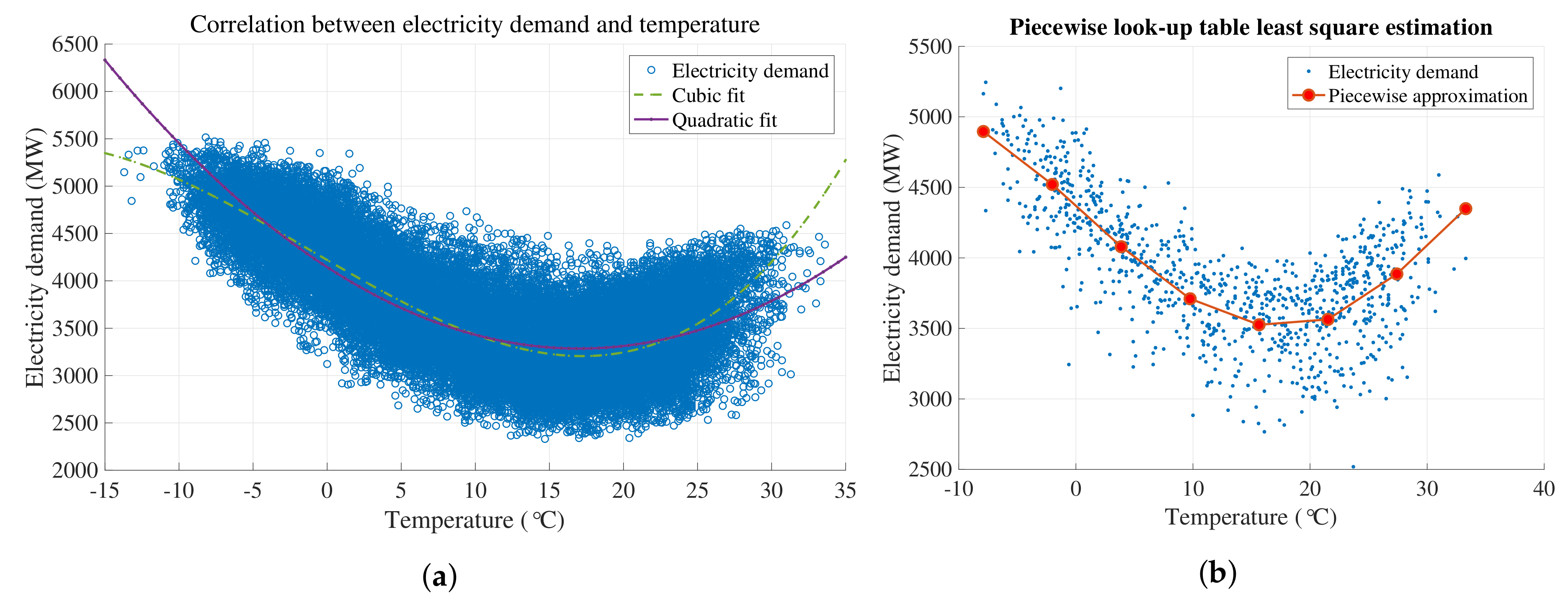
| Hokkaido | Hourly (2013–2015) | 15.65 (HDD), 21.53 (CDD), 17.1 (min. demand) (2 p.m. data) | Piecewise | This study |
| −10.2 (min. exhaustion), 33.18 (max. exhaustion), 16.28 (min. demand) | Polynomial | This study |
| Temperature °C | Hour 1 | Hour 14 | Hour 19 | ||||||
|---|---|---|---|---|---|---|---|---|---|
| CDD_val | Deviation | CDD_val | Deviation | CDD_val | Deviation | ||||
| 19.000 | −5.3611 | −0.0178 | −1.7623 | −3.0000 | −0.0194 | −1.9206 | −1.1465 | 0.0068 | 0.6854 |
| 20.000 | −4.3611 | −0.0119 | −1.1783 | −2.0000 | −0.0134 | −1.3303 | −0.1465 | 0.0165 | 1.6629 |
| 21.000 | −3.3611 | −0.0059 | −0.5909 | −1.0000 | −0.0074 | −0.7365 | 0.8535 | 0.0262 | 2.6498 |
| 22.000 | −2.3611 | 0.0000 | 0.0000 | 0.0000 | −0.0014 | −0.1392 | 1.8535 | 0.0358 | 3.6463 |
| 23.000 | −1.3611 | 0.0059 | 0.5944 | 1.0000 | 0.0046 | 0.4618 | 2.8535 | 0.0455 | 4.6525 |
| 24.000 | −0.3611 | 0.0119 | 1.1924 | 2.0000 | 0.0106 | 1.0664 | 3.8535 | 0.0551 | 5.6684 |
| 25.000 | 0.6389 | 0.0178 | 1.7939 | 3.0000 | 0.0166 | 1.6746 | 4.8535 | 0.0648 | 6.6942 |
| 26.000 | 1.6389 | 0.0237 | 2.3990 | 4.0000 | 0.0226 | 2.2865 | 5.8535 | 0.0745 | 7.7299 |
| 27.000 | 2.6389 | 0.0296 | 3.0077 | 5.0000 | 0.0286 | 2.9021 | 6.8535 | 0.0841 | 8.7758 |
| 28.000 | 3.6389 | 0.0356 | 3.6200 | 6.0000 | 0.0346 | 3.5213 | 7.8535 | 0.0938 | 9.8317 |
| 29.000 | 4.6389 | 0.0415 | 4.2359 | 7.0000 | 0.0406 | 4.1443 | 8.8535 | 0.1034 | 10.8979 |
| 30.000 | 5.6389 | 0.0474 | 4.8555 | 8.0000 | 0.0466 | 4.7711 | 9.8535 | 0.1131 | 11.9745 |
| 31.000 | 6.6389 | 0.0533 | 5.4788 | 9.0000 | 0.0526 | 5.4016 | 10.8535 | 0.1228 | 13.0615 |
| 32.000 | 7.6389 | 0.0593 | 6.1058 | 10.0000 | 0.0586 | 6.0359 | 11.8535 | 0.1324 | 14.1591 |
| Model Types | Overall MAPE (%) | Maximum MAPE (%) | MAPE ≤ 2% | MAPE > 2% | MAPE ≥ 5% | MAPE ≥ 10% | MAPE ≥ 15% | Observations | |
|---|---|---|---|---|---|---|---|---|---|
| Overall | Model A | 2.43 | 19.32 | 53.5 | 46.5 | 11.56 | 1.09 | 0.19 | 8760 |
| Model B | 1.98 | 15.41 | 62.49 | 37.51 | 6.97 | 0.53 | 0.01 | ||
| Model C | 1.72 | 14.06 | 67.93 | 32.07 | 4.05 | 0.23 | 0 | ||
| Working days | Model A | 1.15 | 19.04 | 54.78 | 45.22 | 9.71 | 0.69 | 0.12 | 5784 |
| Model B | 1.03 | 13.8 | 64.93 | 35.07 | 5.53 | 0.32 | 0 | ||
| Model C | 0.90 | 13.35 | 70.35 | 29.65 | 2.71 | 0.172 | 0 | ||
| Weekends | Model A | 2.49 | 11.93 | 52.87 | 47.13 | 12.66 | 0.92 | 0 | 2376 |
| Model B | 2.03 | 11.75 | 60.56 | 39.44 | 7.82 | 0.21 | 0 | ||
| Model C | 1.81 | 9.2746 | 66.28 | 33.71 | 5.57 | 0 | 0 | ||
| Holidays | Model A | 3.52 | 19.33 | 43.5 | 56.5 | 25 | 5.66 | 1.66 | 600 |
| Model B | 2.93 | 15.42 | 46.5 | 53.5 | 17.5 | 3.83 | 0.16 | ||
| Model C | 2.51 | 14.06 | 51.17 | 48.83 | 11.33 | 1.66 | 0 |
© 2018 by the authors. Licensee MDPI, Basel, Switzerland. This article is an open access article distributed under the terms and conditions of the Creative Commons Attribution (CC BY) license (http://creativecommons.org/licenses/by/4.0/).
Share and Cite
Chapagain, K.; Kittipiyakul, S. Performance Analysis of Short-Term Electricity Demand with Atmospheric Variables. Energies 2018, 11, 818. https://doi.org/10.3390/en11040818
Chapagain K, Kittipiyakul S. Performance Analysis of Short-Term Electricity Demand with Atmospheric Variables. Energies. 2018; 11(4):818. https://doi.org/10.3390/en11040818
Chicago/Turabian StyleChapagain, Kamal, and Somsak Kittipiyakul. 2018. "Performance Analysis of Short-Term Electricity Demand with Atmospheric Variables" Energies 11, no. 4: 818. https://doi.org/10.3390/en11040818
APA StyleChapagain, K., & Kittipiyakul, S. (2018). Performance Analysis of Short-Term Electricity Demand with Atmospheric Variables. Energies, 11(4), 818. https://doi.org/10.3390/en11040818


