Performance Analysis of Short-Term Electricity Demand with Atmospheric Variables

Abstract

The quality of short-term electricity demand forecasting is essential for the energy market players for operation and trading activities. Electricity demand is significantly affected by non-linear factors, such as climatic conditions, calendar components and seasonal behavior, which have been widely reported in the literature. This paper considers parsimonious forecasting models to explain the importance of atmospheric variables for hourly electricity demand forecasting. Many researchers include temperature as a major weather component. If temperature is included in a model, other weather components, such as relative humidity and wind speed, are considered as less effective. However, several papers mention that there is a significant impact of atmospheric variables on electricity demand. Therefore, the main purpose of this study is to investigate the impact of the following atmospheric variables: rainfall, relative humidity, wind speed, solar radiation, and cloud cover to improve the forecasting accuracy. We construct three different multiple linear models (Model A, Model B, and Model C) including the auto-regressive moving average with exogenous variables (ARMAX) with the mentioned exogenous weather variables to compare the performances for Hokkaido Prefecture, Japan. The Bayesian approach is applied to estimate the weight of each variable with Gibbs sampling to approximate the estimation of the coefficients. The overall mean absolute percentage error (MAPE) performances of Model A, Model B, and Model C are estimated as 2.43%, 1.98% and 1.72%, respectively. This means that the accuracy is improved by 13.4% by including rainfall, snowfall, solar radiation, wind speed, relative humidity, and cloud cover data. The results of the statistical test indicate that these atmospheric variables and the improvement in accuracy are statistically significant in most of the hours. More specifically, they are significant during highly fluctuating and peak hours.

1. Introduction

Short-term electricity demand or load forecasting is a way of estimating future demand for a short time horizon, commonly an hour to one week ahead. According to the time horizon for prediction, Apadula et al. [1] classified the load forecast into four categories: very short-term forecasts (from a few minutes to 1 h ahead), short term forecasts (from 1 h–1 week ahead), medium-term forecasts (from one week to a year head) and long-term forecasts (longer than a year ahead). Such differences in the lead time influence the choice of models and methods to apply, as well as the selection of important external factors affecting the electricity demand (socio-economic, atmospheric, seasonal and time-dependent factors) [1]. For short-term demand forecasting, we exclude socio-economical factors and consider atmospheric, seasonal and other short-term dependent variables. To avoid an ambiguous presentation, we note that the rest of this paper uses two terms: ‘demand forecasting’ and ‘other weather variables’ to refer to ‘electricity demand forecasting’ and ‘rainfall, snowfall, solar radiation, wind speed, relative humidity, and cloud cover’, respectively.

Knowledge of electricity demand behavior in advance is crucial for the planning, analysis and operation of power systems to assure an uninterrupted, reliable, secure and economic supply of electricity. These days, electric utility industries are undergoing a highly competitive market-driven industry. Every electricity provider is focusing on decreasing power generation cost by increasing the efficiency of load demand management. For the market operator, forecasting is crucial for scheduling and dispatch of generators’ capacity. For electricity generators, the strategic choice involved in bidding and re-bidding of capacity depends on demand forecasts [2]. Such bidding and re-bidding processes determine the market volatility for the electricity price. Similarly, for the electricity retailer, demand forecasting affects the decisions about the balance between the hedging spot acquisition of electricity for consistent energy supplies without black outs and possibly minimum cost. Improving the accuracy of electricity forecast could reduce the power marketing risk and keep the market stable for electricity demand and price, as well [3,4] Therefore, accurate electricity load demand forecasting for different time horizons is a very hot research issue.

Most electric utilities serve residential, commercial and industrial area customers. In residential areas, electricity depends on human activities. Therefore, electricity demand may rise to a peak during the morning and evening. Residential customers are very sensitive to weather fluctuations, but calendar (weekday, weekend, and holiday) effects have very low predictive power [5]. Retail stores, restaurants, hotels and educational institutes are commercial customers, and their demand is affected by business schedules and some weather behavior. This results in electricity demand dropping significantly during weekends or holidays. Industrial customers play a vital role to increase or decrease electricity demand. However their characteristics are also similar to commercial customers and quite difficult to predict. In our study, aggregate demand data are used to analyze the impact of atmospheric variables; therefore, it seems more challenging.

Many authors emphasize univariate models with historical data and perform forecasting with acceptable accuracy [6]. Despite that, [7] suggest that the level of accuracy can be improved by including weather variables. Furthermore, the Intergovernmental Panel on Climate Change (IPCC) suggests that global temperature is gradually increasing, and there is evidence of an increase in the frequency of extremes [8]. These extremes directly affect electricity demand. According to IPCC, global warming has already made the world 0.74 °C warmer over the last 100 years, and temperatures are probably going to increase by 1.8–4 °C by the end of the century. Therefore, many authors have studied the impact of weather on electricity demand [1,7,9,10,11,12,13,14]. Historical data of electricity demand show negative linear effects on load demand during the winter season. The experience of many utilities is that atmospheric variables that cause an influence on electricity demand are temperature, humidity, wind speed and precipitation, in decreasing order of importance [15]. This conclusion is drawn from the study of a considerable number of atmospheric variables on electricity demand for Greece for better forecasting performance. All these scenarios envision that electricity demand essentially depends on meteorological variability [1]. However, only temperature is considered as the most essential variable [7,16,17]. There are three main reasons behind excluding other weather variables: (i) they show lower impact on electricity demand [18]; (ii) it is expensive to install weather stations to collect all these data; and (iii) there are potential collinearity problems when simultaneously employing several weather variables as explanatory variables [16]. However, our main concern in this paper is to analyze the impact of these other weather variables to enhance forecasting performance because [6,7,17] strongly recommended that including meteorological variables can improve forecasting accuracy.

An appropriate modeling technique in demand forecasting is crucial for high accuracy and stable performances. In short-term load demand forecasting, the well-cited papers [2,5,7,12,14,19,20,21,22] implemented statistical techniques especially multiple linear regression (MLR), semi-parametric and ARMAX models. Similarly, artificial intelligence techniques especially artificial neural network (ANN), fuzzy and support vector machine (SVM) models were implemented in [9,10,23,24,25]. Several modeling concepts for robust parameter estimation used prior to 1990 were discussed in [26], and it was concluded that MLR was superior. Interest in ANN modeling for electricity demand forecasting began in 1990 because of its fairly good results. Nevertheless, these good results were due to the ability to peek into the future and undergo over-fitting due to either over-training or over-parameterization [27]. For example, the non-linear autoregressive ANN model was implemented in [25] and achieved 30% improvement on the average error compared to traditional ANNs, ARMAX and state space models. In fact, ANNs are black-box techniques, and they do not offer insights into the relation between electricity demand and driving factors. Hippert et al. [23] analyzed 40 papers and concluded that without solid support, ANNs are good enough for short-term demand forecasting. Chow et al. [10] agreed that MLR models are capable of characterizing the relationship between load demand and other exogenous factors, but this is a complicated modeling technique and requires enormous computational effort to produce acceptable results. Various time series models such as seasonal autoregressive integrated moving average (SARIMA) and the SARIMA model with exogenous variables are not able to react fast enough to rapid demand changes that deviate from the historical demand forecast [5]. The MLR model with a dynamic error structure and adaptive adjustment of forecasted error proposed in [19] was the winner of a load forecasting competition organized by a utility in the U.S. Hong et al. [28] reviewed the modeling techniques of winning teams in the Global Energy Forecasting Competition 2012 (GEFCom2012), where all four wining teams applied regression analysis, while only two teams implemented ANN. Apart from neural nets, other traditional and adaptive techniques such as SARIMA and regression ARIMA (RegARIMA) have been compared to linear regression for cognate energy prediction with weather variable selection. The result showed that linear regression was highly effective and better than other sophisticated techniques for the majority of simulations in [29]. Therefore, more robust modeling techniques comprise our concern to handle the chaotic behavior of atmospheric variables.

Three different scenarios are discussed in this paper before drawing some conclusions. In the first scenario, an MLR as the ARMAX model with deterministic variables, historical demand and the interaction of days with historical demand data was constructed and named Model A. In the second scenario, temperature-derived variables and their interaction with months were added to Model A, and this new model was named Model B. Similarly, in the third scenario (named Model C), other atmospheric variables were added to Model B. These models were trained with a rolling window of two years of data and forecasted for one year out from the sample data. Finally, we interpreted the impact and significance of weather variables for short-term demand forecasting and also compared the forecasting accuracy among these three models.

This paper contributes to short-term demand forecasting by showing that atmospheric variables, such as relative humidity, wind speed, rain fall, solar radiation, and cloud cover, improve the accuracy, compared to the baseline models Model A, Model B, and Model C with temperature (alone) for Hokkaido Prefecture. Analysis of the individual impacts of the atmospheric variables is also a crucial contribution. We believe that the selection of the best weather stations and estimation of the exhaustion temperatures, the base temperatures for cooling degree days (CDD) and heating degree days (HDD) comprise a pioneer work for short-term electricity demand forecasting in Hokkaido Prefecture, Japan. No published study to our knowledge has taken an MLR approach with an ARMAX modeling for short-term demand forecasting in Hokkaido Prefecture.

The organization of this paper is as follows. Section 2 describes the characteristics of electricity demand data, and atmospheric variables are discussed. Different modeling techniques, methodologies and results related to this paper are presented in Section 3. Section 4 demonstrates an extensive empirical analysis of variables for the quality of the model fit for our dataset. An estimation and a forecasting technique followed in this paper is discussed in Section 5. Section 6 deals with the comprehensive discussion of the predicted results and analysis, and Section 7 concludes this paper.

2. Description of Data

The data comprise hourly electricity load demands from the area covered by the utility named the Hokkaido Electric Power Company (HEPCO), ranging from 1 January 2013 to the last day of 2015. The same period of the atmospheric dataset from Japan Meteorological Agency (JMA) is used for this study, which is freely available. There are no missing data on electricity demand, but some missing snowfall, and cloud data are filled up using the interpolation technique. The dataset then is separated into 24 subsets, each containing the load for a specific hour of the day, and used as single series. Such an hour-by-hour approach has been implemented by [19] and won a load forecast competition.

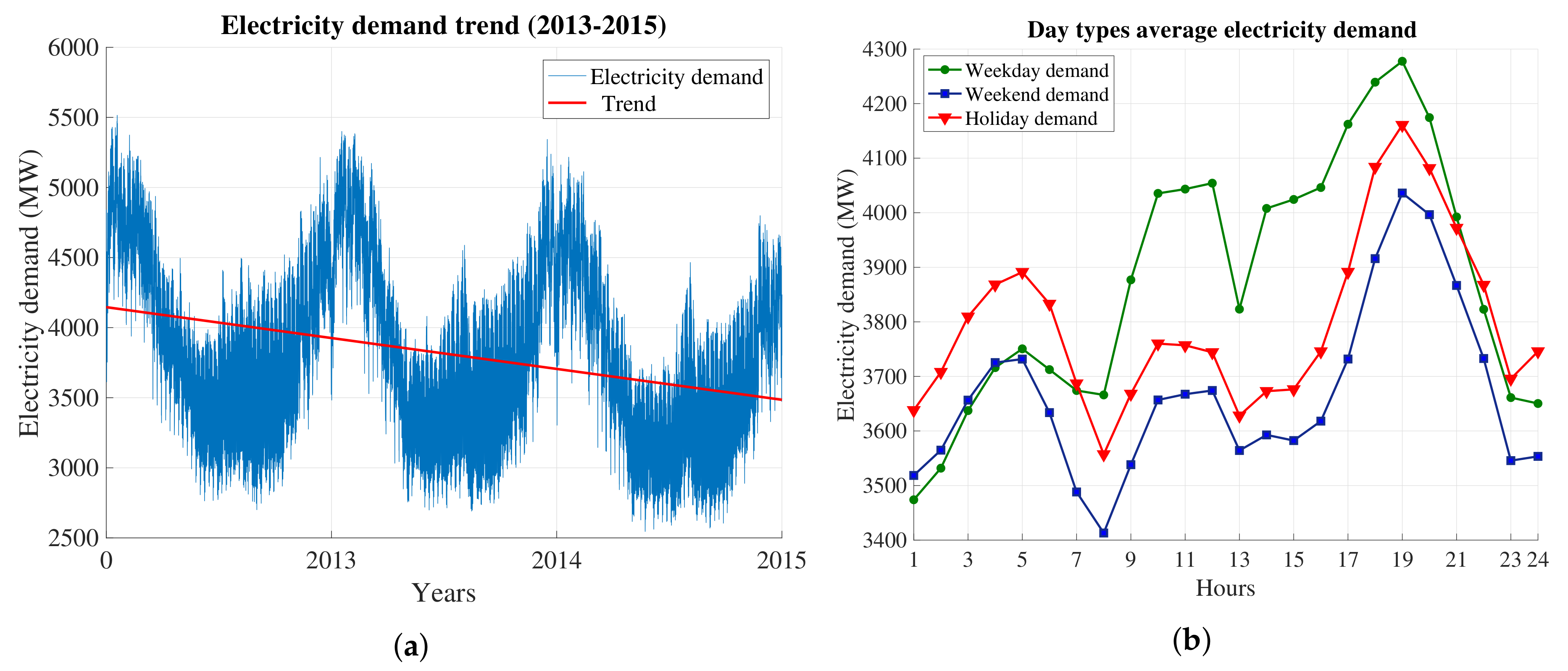
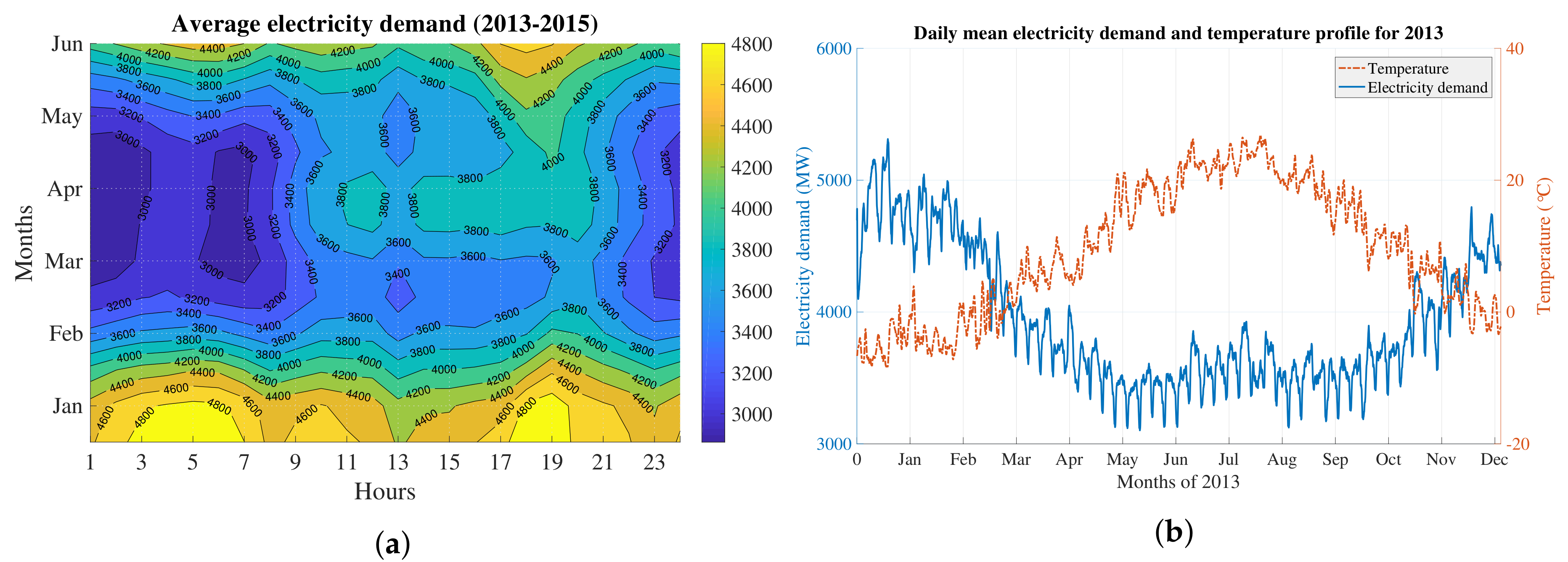
2.1. Electricity Demand Data

Hourly data of 26,280 samples are made available by HEPCO, Japan. Unlike many other countries, HEPCO electricity data exhibit a significant and persistent downward trend (Figure 1a), which is mainly associated with the economic, demographic and population growth of the country. Firstly Japan is already at the saturation level of development and has negative population growth. Secondly, people are shifting their interest towards renewable energy and implementing a smart switching system for residential and commercial buildings. Strong weekly and monthly seasonal patterns are superimposed on this yearly trend (Figure 2b) and are highly correlated with atmospheric factors, especially temperature. Hokkaido is a very cold region; therefore, the peak level of demand occurs during December–February (winter). During this season, the average temperature drops down to −5 °C, causing intensive use of electric heating appliances.

Figure 1b shows the day type variation of electricity demand for all hours with various peaks. After midnight, electricity demand starts to rise until morning Hour 5. On holidays, people enjoy holiday activities during night hours. Therefore, demand rose to the maximum level on holidays. As was our expectation, electricity demand on weekdays dramatically rose after Hour 8 due to office hours and dropped again during lunch hours (noon to Hour 13). However, during the weekend, electricity demand significantly dropped to the minimum level at Hour 8 and slightly rose during the day time. The pattern of rising or falling electricity demand for all days is the same during day hours, and the peak is at Hour 19.

The contour plot in Figure 2a illustrates the details of average electricity demand for all hours of the day and all months of the year from 2013–2015. During the winter season, especially the last week of December to the first week of February, there are two peaks of demand in the morning and evening time. Morning peaks exist from Hour 4–Hour 6 and an evening peak approximately from Hour 18–Hour 19 of 4800 megawatts (MW) in magnitude. However, in the summer season, the demand level dramatically falls to an extreme low during the morning time. Since Hokkaido Prefecture suffers from a very cold climate during the winter season (30-year mean temperature in January: −8 °C), people use electricity for warming purposes such as room heating, building heating, and water heating. Furthermore, the variation of the pricing and the needs of people cause excessive demand during the morning and evening time. The lowest demand for a similar time period is found in June, but soon after, a significant rise in temperature causes electricity demand to rise again until August, which is the hottest month (30-year mean temperature in August: 22 °C). This is exactly the opposite reason that causes and exhibits seasonal variation to that of winter (Figure 2b).

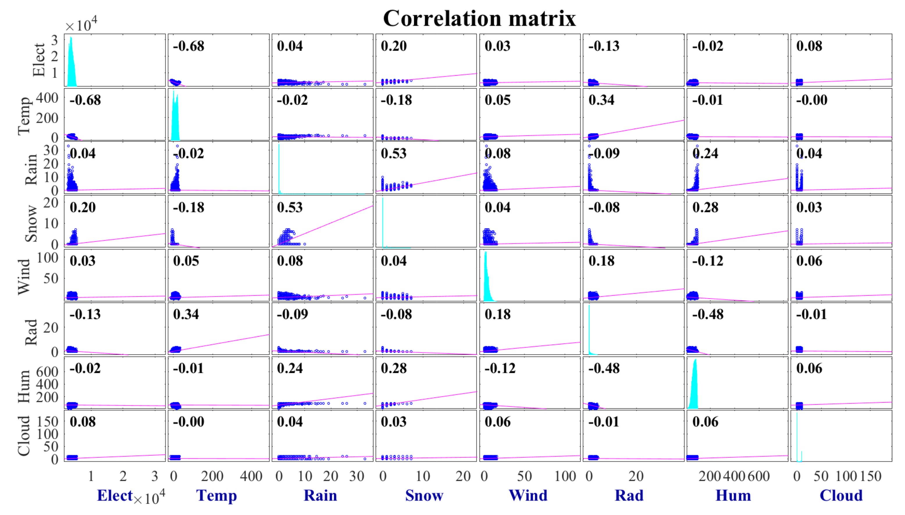
2.2. Atmospheric Variables

The climate of Japan is showing long-term changes, and the frequency of extremes of maximum temperature is increasing, as well as annual temperature is expected to increase. A good review paper about the impact of climate change for energy consumption [30] discussed the demand for energy, coal, gas, oil and electricity for Japan. The paper concluded that energy consumption was responding according to the variations in temperature. The higher the temperature, the higher will be the consumption during the summer in warmer countries; and the lower the consumption during winter in colder countries. This is unlike [30], because the cold region Hokkaido, Japan, shows a higher demand during winter. Therefore, the analysis of the impact caused by following atmospheric variables is of interest for short-term demand forecasting: Temperature contributes the most to the majority of load forecasting variations in electricity demand. Increased temperature during the winter will reduce electrical heating load. Conversely, in the summer, electrical heating is normally absent, but high temperatures increase the refrigeration and air-conditioning load. Wind speed may have some effects on air conditioning and cooling fans because of air chill. However, its effect is relatively localized. Rainfall also shows a localized impact on electrical heating demand similar to wind speed. If it is raining, there must be cloud cover, no radiation and the possibility of wind, as well. Therefore, these atmospheric variables are intra-correlated among themselves. Wet conditions can affect the efficiency of air-vented dryers and can be considered as the effect of relative humidity. This means that during the periods of high humidity, electricity demand tends to increase. However, in Hokkaido region, electricity demand decreases with the increment of humidity in the summer (

Table 1. Correlation coefficients of weather variables with electricity demand.

Variables	Winter (January)	Summer (August)
Temperature	−0.3495	0.5302
Rain	0.0727	−0.0078
Humid	0.1385	−0.4348
Radiation	−0.2321	0.4141
Snow	0.1013	No snowfall data

) and vice versa in the winter. Cottet and Smith [20] resolved the nonlinearity issue by the interaction of temperature and humidity. Besides the relative humidity, an increase in cloud cover can also increase demand for lighting purposes. Recorded hours of sunshine in a period are a more direct indicator of cloud cover. In this study, forecast models are trained and tested using measured atmospheric data instead of forecasted data.

From three years of sampled data, we have plotted the correlation matrix of all weather-related explanatory variables of electricity demand in Figure 3. There is a positive correlation of electricity demand with rainfall, snowfall, wind speed, and cloud cover, i.e., the increase of rainfall, snowfall, wind speed, and cloud cover causes an increase in electricity demand. However, there is a very high negative correlation with temperature (−0.68), indicating that the overall temperature in Hokkaido is cold, and this cold causes an increase in electricity demand.

We can notice that other weather variables, except temperature, have a small correlation with electricity demand, indicating a lower impact on electricity demand. This is one reason why many researchers have used only temperature as the weather variable. The collinearity problem [16] is another reason for ignoring these weather variables, if temperature is already used in the model. This is because the temperature is expected to be correlated with radiation, cloud cover, and wind speed, as well. Furthermore, weather variables are correlated among themselves. For example, if there is rainfall, there is the possibility of cloud cover, humidity, wind speed, and snowfall.

The correlation of atmospheric variables with the electricity demand is measured in Table 1. For both seasons, temperature is the factor most correlated with electrical demand. Solar radiation has a negative correlation during the winter season, while it has a positive one during the summer. In the winter time, a significant lighting and heating load coincides with the lower temperatures; therefore, the solar radiation tends to provide warmth, resulting in less use of heating appliances. Conversely, in the summer, demand tends to increase because of solar radiation. Similarly, relative humidity and precipitation show a positive correlation during the winter and the opposite in the summer. However, Solar radiation and relative humidity during the summer show approximately equal and opposite correlation results with minimization of their individual effects, and a strong correlation of temperature remains a dominant factor for electricity demand during the summer.

Since there is a strong correlation between electricity demand and temperature, special analysis of this relationship is required. In the Hokkaido data, it can be seen that there is a strong non-linear relationship between demand and temperature (Figure 4). Electricity demand is increasing for an increase or decrease of temperature from a certain point known as the base temperature. It is reported in the literature that the base temperature varies from 12.9–22 °C (

Table 2. Base temperature summary from some published studies.

Region	Electrical Data	Base Temperature (°C)	Relationship	Reference
USA	Weekly	18.3	Linear with CDD	[32]
Spain	Daily (1983–1999)	18.5	Non-linear	[33]
Italy	Hourly (2002–September 2003)	18.7 (HDD), 22 (CDD)	Linear with CDD, HDD	[34]
London	Hourly (1997–2001)	16	CDD HDD	[21]
South Korea	Monthly (2001–2010)	16.2–19.4	CDD HDD	[35]
Tokyo	Hourly	15 (HDD), 21.3 (CDD)	Piecewise	[36]
Tokyo	2 p.m. data	17.25	Piecewise	[37]
Brisbane	Half-hourly	18.6	Linear with CDD, HDD	[38]
Sydney	Weekly (1999–2000)	17.5	Linear with CDD, HDD	[38]
Melbourne	Weekly (1999–2000)	16.9	Linear with CDD, HDD	[38]
Adelaide	Weekly (1999–2000)	16.8	Linear with CDD, HDD	[38]
Hokkaido	Hourly (2013–2015)	15.65 (HDD), 21.53 (CDD), 17.1 (min. demand) (2 p.m. data)	Piecewise	This study
		−10.2 (min. exhaustion), 33.18 (max. exhaustion), 16.28 (min. demand)	Polynomial	This study

). Some industrial sectors use a very low base temperature (e.g., refrigerators or department stores). Local outdoor cooling sources and adaption to human comfort levels may cause these large variations of the base temperature [31].

The relationship (Figure 4) between temperature and electricity demand is usually asymmetric. Therefore, third or higher order polynomial models are preferred to determine the base temperatures for minimum electricity demand and exhaustion point(s) (one or more points), rather than the second order polynomial. In this paper, we implement two techniques: (i) polynomial models (2nd, 3rd, 4th and 5th); and (ii) piece-wise linear models, as mentioned in Table 2. There is an approximately constant slope of electricity demand, no matter how much the temperature drops from −10.2 °C and no matter how increased from 33.18 °C. These two points are defined as exhaustion points. Similarly, the base temperature for minimum demand is observed at 16.28 °C. This point is important because there is no effect of temperature on electricity demand. However, our piece-wise linear model evaluates this point at 17.1 °C, from 2 p.m. data.

In piece-wise linear approximation, 2 p.m. demand from weekdays is used. The least squares estimation technique is used to approximate HDD and CDD points by varying the number of knots (3–30) from minimum to maximum temperature. From the eight knots’ (at temperatures of −7.9 °C, −2.01 °C, 3.87 °C, 9.75 °C, 15.64 °C, 21.53 °C, 27.41 °C and 33.3 °C, i.e., seven linear pieces) look-up table, where the fifth spline in Figure 4b explains the temperature between 15.65 °C and 21.53 °C, exhibit base temperatures. In this temperature range, electricity demand has a negligible response to the variation of temperature. Therefore, we implement these two points as base temperature points to calculate HDD and CDD for our further calculation.

2.3. Weather Station Selection

JMA has installed 226 automated weather stations at different location of Hokkaido Prefecture. Our interest is to observe the most effective weather station concerning electricity demand variation. In this paper, a combination of three weather stations with the simple mean is used because of the lower MAPE and lower variance values. The three selected stations are the regional headquarter weather stations of Sapporo, the special automated weather station of Hakodate and Kitami. The details of the methodology are explained in Appendix A.

3. Related Works

In the literature, many authors have developed a model without any exogenous variables. Even so, they show competitive forecasting performance with many multivariate models. For example, Taylor [6] employed double seasonal exponential smoothing for half hour data and predicted very good results with MAPE of 1.2–2% for half hour to day ahead lead time forecasting. Nevertheless, only historical demand dataset may not sufficiently address the effect on electricity demand because temperature variation is also an important factor that directly influences electricity demand. Harvey and Koopman [39] used a time-varying splines model with temperature to get MAPE performance up to 3%. After 2003, climate change has been affecting the variation of demand such as modification of the annual daily load curve and shifting of the peak demand occurrence from evening to morning in Jordan [14]. In Europe, extremely high temperatures during the summer of 2003 created significantly greater electricity demand. Ihara et al. [36] reported that a 1 °C rise in temperature was equivalent to a 180-MW increment in electricity demand for Tokyo, Japan. They also studied the impact of other weather variables for peak demand forecasting. The recent paper by Staffell and Pfenninger [40] concluded that electricity demand and supply are becoming increasingly weather dependent in the U.K. In [31], weather sensitivity for short-term prediction of electricity demand was analyzed for warm working days for Adelaide, Australia. For a long lead time forecasting model, weather prediction shows higher uncertainty, but for a short lead time level of uncertainty is very low. Therefore, Trotter et al. included weather uncertainty for demand forecasting in Brazil [22]. Apadula et al. [1] mentioned the role of various weather-related components quantitatively for electricity demand in Italy. Lusis et al. mentioned that the atmospheric effect on demand is significant [5].

Weather variables, such as temperature and humidity, were employed for modeling electricity load consumption in [20], and it was concluded that including these variables yields better results with consistent performance. Factors affecting electricity demand in Athens, Greece, and London were studied in [21]. They compared both weather and non-weather factors and found that temperature is the most sensitive for electricity load demand, especially in Athens. Satish et al. [41] studied the effect of temperature with 20 training patterns and compared the results, but there is no comprehensive analysis with atmospheric variables. Friedrich and Afshari [42] investigated the results for Abu Dhabi city electricity load using multiple weather variable for a 24 h–48 h prediction horizon and obtained a very promising result of 1.5% MAPE. Apadula et al. [1] analyzed weather and calendar variables affecting monthly electricity demand using an MLR model for Italy and concluded that the calendar component considerably contributed from January–May with 4–7.7%. The contribution of the cooling degree months ranges from 3.4–7.6% during the summer months, while the heating degree months of winter months was lower. The influence of the cloud cover variable is always below 1% throughout the year. They improved monthly demand forecast by 1.3% by including atmospheric variables. However, individual atmospheric variables were not analyzed comprehensively.

Exploring the link between electricity use and temperature is important to assess the impact of climate change on energy demand. Ongoing climate changes have promoted an increased scientific interest in the study of the relationships between energy consumption and weather variables. Similar to our result, [1] for Italy [43] and [12] for the European region concluded that including all weather-related variables can give the lowest MAPE, but the improvement in accuracy was usually smaller. In [12], the European region is classified based on their average monthly temperature into three groups: cold, intermediate and warm. Cold countries demonstrated almost a linear relationship with only heating components. For intermediate countries, the cooling component is clearly visible though dominated by the heating component. Warm countries presented a highly non-linear relationship with a cooling component of a similar scale as heating for Adelaide [31] and explained that for Japan [36]. When wind speed is above some value, electricity usage is increased for heating in the winter as it increases the feeling of coldness when temperatures are low. For summer, the correlation between wind speed and electricity demand is not clearly visible. The value of humidity is reported to matter only if it coincides with the specified value of other variable. The feeling of hotness accompanying temperatures above certain value is intensified by high humidity, which can increase energy use for air conditioning. Xie et al. [17] included relative humidity in their model to improve relative accuracy by 21% in North Carolina. In [10], the weather variables that cause a significant impact on electricity demand for Hong Kong were discussed. The effect of wind cooling exterior walls of buildings was intensified if they were wet. For regions with a certain climate, usage of humidity was reasonable [10]. This weather compensation neural network model was capable of providing more accurate forecasts with a 0.9% reduction in forecasting error for Hong Kong.

Therefore, it is worth examining the influence of each atmospheric variable for short-term electricity demand forecasting. This is because there is always a research gap for the statistical analysis of accuracy improvement and the significance of other individual atmospheric variables in the literature of demand forecasting. However, in real-time forecasting systems, we must implement forecasted weather data instead of measured data, as they always contain some error. Fay and Ringwood [44] studied the effect of weather forecast error while implementing a short-term load forecasting model. Their tested results showed that weather forecast error causes an approximately 1% deterioration in accuracy.

4. Prototype Modeling

4.1. Modeling Trend

The existence of a trend largely depends on the length of the time period examined, industrialization and rapid economic growth. Electricity load data have occasionally been found to be non-stationary. The use of the logarithm or the performance difference of the historical data is applied to account for the non-stationarity. However, fitting a deterministic trend in the model is more appropriate rather than the difference. The seminal paper of Ramanathan et al. [19] fitted both a linear trend and the reciprocal of that to their model. In this paper, the logarithm is used for historical demand data to avoid possible heteroscedasticity and trend adjustment. The positive integer is also included in the model, but the estimated weight is almost zero, indicating that taking the logarithm of historical data had already captured the trend.

4.2. Modeling Cyclicality and Seasonality

A cyclic pattern exists when data exhibit rises and falls, but not in a fixed period. However, a seasonal pattern exists when a series is influenced by seasonal factors, such as the quarter of the year, the month or the day of the week. Therefore, seasonality is always of a fixed and almost known period. Unlike seasonal behavior, cycles no longer occur, but there is more variation of the magnitude. The class of ARMA models can handle both seasonality and cyclic behavior. An $ARMA(p,q)$ model can be cyclic if $p>1$. Therefore, ARMA models have been extensively applied in the load forecasting literature [45,46]. The most popular time series techniques that have been adopted are ARMA or ARMA with exogenous variables (ARMAX) models. However, a long period of cyclicity is not handled very well. According to Hahn et al. [47], time series load data contain three seasonal patterns: intraday (daily), weekly and annual, which is quite similar to electricity price data. Silvano et al. [48] mentioned that electricity demand and price exhibit a strong daily seasonality due to day and night hours and weekly seasonality due to working and non-working days.

A lag structure-based model for MLR is constructed to capture seasonality because lag structures alone cannot capture the complete seasonal features during weekends [49]. The reason is explained by Clements et al. [2]: the electricity demand for Saturday and Sunday was significantly over-predicted (negative bias in the errors). This stems from the fact that a higher load on a weekday is being used as a one-day lagged load in generating the forecast for weekends. Similarly, when the Sunday load is used in generating the forecast for Monday, significant under-prediction occurs (positive bias in the errors) [2]. Essentially, this bias is due to the fact that the coefficients on one-day lagged load do not differentiate between days of the week. A simple way to deal with this issue is to combine the one-day lagged load with day-of-the-week dummy variables. However, our models avoid this step because of the excessive number of variables.

4.3. Mathematical Model

Since sampling of the data is performed every hour, there are N = 24 samples in a day. We separate these samples’ hour-wise pattern to forecast the electricity demand for the first hour of the day by one equation and the second for the second hour of the day from the next equation, and so on. Hence, we need 24 individual equations for a one-day forecast, and now, the generic prototype model is,

$$\begin{array}{cc}\hfill D_{h,d}& =De{t}_{h,d}+Atm{V}_{h,d}+DHis{t}_{h,d}+ITerm{s}_{h,d}+v_{h,d}\hfill \end{array}$$

(1)

In Equation (1), predictor variables are grouped as deterministic, atmospheric, historical electrical demand and interaction terms, denoted by $Det$, $AtmV$, $DHist$ and $ITerms$, respectively, for hour of day h and forecasting days d. The residual $v_{h,d}$ modeling is very sensitive and important in MLR because of the incorporation of an auto-regressive structure in the error term. According to the econometric regression theory, if the residuals are serially correlated, the estimation of coefficients may lead to instability and cause misleading results. Therefore, Equation (2) assumes that the current value of the error term at hour h of day d is denoted by $v_{h,d}$, i.e., error terms are assumed to follow an autoregression in previous days and are modeled as the sum of the finite order of previous errors. This paper has treated each hour as a separate time series; therefore, the correlation error between hour can reasonably be taken as small [19]. Mathematically,

$$v_{h,d}=\sum _{i=1}^q{\rho }_{h,i}{v}_{h,d-i}+{ϵ}_{h,d}$$

(2)

for $h=1,\dots ,24$. The term $v_{h,d-i}$ is the serially-correlated error term up to q lags. The simple Ljung–Box Q-test can be implemented for selecting the appropriate order of q and ${ϵ}_{h,d}=N(0,{\sigma }^2)$.

The term $De{t}_{h,d}$ refers to predictable variables that can capture the seasonality of electricity demand, where demand variation is based on a day of weeks, a month of years and years. The historical demand profile shows higher demand during the business week (Monday–Friday) than that of weekends (Saturday and Sunday) and public holidays. Such an effect can be addressed by dummy variables. The number of dummy variable selection criteria for weekdays $dv=7$ and for months $m=12$ is $dv-1$ and $m-1$, respectively. If all dummies ($dv=7$ and $m=12$) are used in the regression together with the intercept, then this set of dummies is linearly dependent on the intercept called the perfect multicollinearity or dummy variable trap and affects the stability of the regression coefficients [50]. Therefore, six dummy variables $W{D}_{h,d}^i$ where $i=1,\dots ,6$ represent the corresponding days of the week ($i=1$ for Sunday, $i=2$ for Monday, ..., $i=6$ for Friday), except Saturday. Because, Saturday is considered as a reference day. Each dummy variable has only two allowable values, either zero or one. For example, if the day d is Monday, then the variable $W{D}_{h,d}^2$ takes the value one, while all other variables $W{D}_{h,d}^i$ are zero. Similarly, if the day d is Sunday, then all the variables $W{D}_{h,d}^i$ take the value zero, except $W{D}_{h,d}^1$. Now, the days’ dummy variables are explained as,

$$W{D}_{h,d}^i=\left\{\begin{array}{cc}1\hfill & \mathrm{if}daydisDay\left(i\right)\hfill \\ 0\hfill & otherwise\hfill \end{array}\right.$$

(3)

where $Day\left(1\right),\dots ,Day\left(6\right)$ represent Sunday, ..., Friday, respectively. Additionally, the linear function of the dummy variables can be written as $W{D}_{h,d}={\sum }_{i=1}^{dv-1}{\beta }_{i}W{D}_{hd}^i$. Some other categorical variables such as working day after a holiday, working day before a holiday and long holidays are also included in the $De{t}_{h,d}$ modeling as dummy variables. Therefore, the model $De{t}_{h,d}$ is formulated with 26 variables, including constant ${\beta }_0$. For simplicity, we use variable vector $\mathit{\beta }$ for all the coefficients.

For the months’ dummy variables, eleven dummy variables ($M_{hd}^j$) where $j=1,\dots ,11$ in the model account for the monthly seasonality of electricity demand, not only related to the weather conditions. Monthly seasonality of electricity demand may be influenced by a number of economic and social factors such as summer vacations and the seasonal character of some industrial activities. The index j values represent correspondingly all months in a year ($j=1$ for January, $j=2$ for February and $j=11$ for November), except the base month of December. The variable $M_{hd}^j$ takes the value of one if the j observation belongs to the month j, otherwise $M_{hd}^j$ takes zero. Therefore, months’ dummy variables can be formulated as,

$$M_{h,d}^j=\left\{\begin{array}{cc}1\hfill & \mathrm{if}daydisMonth\left(i\right)\hfill \\ 0\hfill & otherwise\hfill \end{array}\right.$$

(4)

where $Month\left(1\right),\dots ,Month\left(11\right)$ represent January, ..., November, respectively. Therefore, the linear function of the dummy variables can be written as $M_{h,d}={\sum }_{j=1}^{m-1}{\beta }_i{M}_{h,d}^j$.

Hence, the term $De{t}_{h,d}$ can be formulated as,

$$\begin{array}{cc}\hfill De{t}_{h,d}& ={\beta }_0+{\beta }_{1}Trend+\sum _{i=2}^7{\beta }_{i}W{D}_{h,d}+\sum _{i=8}^{18}{\beta }_i{M}_{h,d}+{\beta }_{19}W{K}_{h,d}\hfill \\ & +{\beta }_{20}WKBf{H}_{h,d}+{\beta }_{21}LH+{\beta }_{22}WKAf{H}_{h,d}\hfill \end{array}$$

(5)

Here, all the coefficients are carried by vector $\mathit{\beta }$, where ${\beta }_0$ represents the intercept, ${\beta }_1$ is the trend and ${\beta }_i,i=2,\dots ,7$ is for the day of the week dummy variable. Similarly, $i=8,\dots ,18$ for the month of the year dummy variable, and $i=19,\dots ,22$ for working days, a working day before a holiday, a working day after a holiday and long holidays, respectively.

The term $Atm{V}_{h,d}$ is another group of variables that affects the demand of electricity. Some pre-processing of temperature helps to observe the non-linear influence on electricity demand (Figure 2 and Figure 4a,b, which implies 17.1 °C as the reference point where there is no effect of temperature (dead zone) for demand. The base temperatures for HDD and CDD were estimated as 15.65 °C and 21.53 °C, respectively. This means that the temperature between 15.65 °C and 21.53 °C has no effect on electricity demand. However, this may not be true in the realistic observation of months and seasons. Human behavior is different according to the season. For example, humans at 16 °C during the winter season still feel cold and want to use a heater; however, during the summer season, 16 °C is a very comfortable temperature for the human body, and people never use a heater at this temperature. The same situation holds true for 22 °C in the summer season. Therefore, the interaction of CDD with months and the interaction of HDD with months seems necessary to address this realistic problem. A simple rule setup for CDD and HDD is as follows,

$$\begin{array}{cc}\hfill HDD& =max(T_{ref}-T_{d,h},0)if{T}_{d,h}\le 15.65\hfill \\ \hfill CDD& =max(T_{d,h}-T_{ref},0)if{T}_{d,h}\ge 21.53\hfill \end{array}$$

(6)

The heating and cooling effect of the previous day is considered in the model as $HDDDa{y}_{d-1}$, $CDDDa{y}_{d-1}$. The representations of CDD and HDD for daily, maximum and minimum temperature are written as $CDDDay$, $HDDDay$, $CDDmax$, $HDDmax$, $CDDmin$, $HDDmin$, respectively. Similarly, the daily and hourly deviation of temperature are also added to model as $TDevDay$ and $TDevHr$.

Therefore, only temperature-derived terms $AtmV{T}_{h,d}$ consist of the following 16 variables,

$$\begin{array}{cc}\hfill AtmV{T}_{h,d}& ={\beta }_{1}CD{D}_{h,d}+{\beta }_{2}CD{D}_{h,d}^2+{\beta }_{3}CD{D}_{h,d}^3+{\beta }_{4}HD{D}_{h,d}+{\beta }_{5}HD{D}_{h,d}^2+{\beta }_{6}HD{D}_{h,d}^3\hfill \\ & +{\beta }_{7}CDDDa{y}_{h,d}+{\beta }_{8}HDDDa{y}_{h,d}+{\beta }_{9}CDDDa{y}_{h,d-1}+{\beta }_{10}HDDDa{y}_{h,d-1}\hfill \\ & +{\beta }_{11}CDDma{x}_{h,d}+{\beta }_{12}HDDma{x}_{h,d}+{\beta }_{13}CDDmi{n}_{h,d}+{\beta }_{14}HDDmi{n}_{h,d}\hfill \\ & +{\beta }_{15}TDevH{r}_{h,d}+{\beta }_{16}TDevDa{y}_{h,d}\hfill \end{array}$$

(7)

Other atmospheric variables are also accounted for by the mathematical formulations. The weight of ${\beta }_i,i=1,\dots ,11$ represents the coefficient values for these weather variables. Therefore, Equation (7) is added to the new model, and there will be 27 (temperature related: 16: and other atmospheric related: 11) variables combined in the atmospheric model,

$$\begin{array}{cc}\hfill Atm{V}_{h,d}& =AtmV{T}_{h,d}+{\beta }_{1}Rai{n}_{h,d}+{\beta }_{2}Ra{d}_{h,d}+{\beta }_{3}Win{d}_{h,d}+{\beta }_{4}Hu{m}_{h,d}\hfill \\ & +{\beta }_{5}HumDe{v}_{h,d}+{\beta }_{6}RainDa{y}_{h,d}+{\beta }_{7}SnowDa{y}_{h,d}+{\beta }_{8}WindDa{y}_{h,d}\hfill \\ & +{\beta }_{9}RadDa{y}_{h,d}+{\beta }_{10}HumDa{y}_{h,d}+{\beta }_{11}CloudDa{y}_{h,d}\hfill \end{array}$$

(8)

It is obvious that the next day demand level is correlated with its previous day demand from the observation of the historical demand pattern. However, the Ljung–Box Q-test is the simplest method for the correlation test, and in our test, the null hypothesis is rejected. Therefore, we have to accept that there is a significant correlation with the previous day’s demand. Since the auto-regressive (AR) component captures the pattern of load in hour $h=i$ for any given day, it gives a good indication that the load will be higher in hour $h=i$ on the following day(s). Hourly plots of auto-correlation and partial auto-correlation indicate that demand is strongly correlated with day ahead, same time load and previous hour load. Hence, the amount of electricity demand that depends on its previous demand is denoted by $DHis{t}_{h,d}$, and the logarithm is taken (Section 4.1) for historical demand $DHis{t}_{h,d}=ln\left(D_{h,d}\right)$; then, AR structure is modeled as,

$$\begin{array}{cc}\hfill DHis{t}_{h,d}& ={\beta }_1{D}_{h,d-1}+{\beta }_2{D}_{h,d-2}+{\beta }_3{D}_{h,d-7}+{\beta }_{4}Max{D}_{h,d-1}\hfill \\ & +{\beta }_{5}Min{D}_{h,d-1}+{\beta }_{6}D12pmM{A}_{h,d-1}\hfill \end{array}$$

(9)

In Equation (9), the same hour of yesterday’s demand, the day before yesterday’s demand, last week’s demand, yesterday’s maximum demand, yesterday’s minimum demand and the seven-day moving average of midnight demand are denoted as, $D_{h,d-1}$, $D_{h,d-2}$, $D_{h,d-7}$, $Max{D}_{h,d-1}$, $Min{D}_{h,d-1}$, $D12pmM{A}_{h,d-1}$, respectively. The forecasting demand during Saturday and Sunday (weekends) is significantly higher with a negative bias in the errors. This is because the higher load during Thursday and Friday (${\beta }_{1}De{m}_{h,d-1}$, ${\beta }_{2}De{m}_{h,d-2}$) is used to forecast weekends’ demand. Similarly, when Saturday and Sunday demands are used to predict Monday demand, significant under-prediction with positive bias in the errors occurs. To overcome this issue, the interaction between day types and electricity demand (Equation (10)) of that day is necessary.

$$\begin{array}{cc}\hfill DH{I}_{h,d}& =\sum _{i=1}^{24}{\Pi }_{j=1}^6{\beta }_{ij}W{D}_j\times D_{i,d-1}+\sum _{i=1}^{24}{\Pi }_{j=1}^6{\beta }_{ij}W{D}_j\times D_{i,d-2}\hfill \end{array}$$

(10)

Similarly, temperature also shows seasonal characteristics with months; therefore, it is meaningful to combine temperature-derived variables (CDD and HDD) with month dummy variables. It consists of 22 variables.

$$\begin{array}{cc}\hfill TIn{t}_{h,d}& =\sum _{i=1}^{11}{\beta }_i{M}_{h,d}\times CD{D}_{h,d}+\sum _{i=1}^{11}{\beta }_i{M}_{h,d}\times HD{D}_{h,d}\hfill \end{array}$$

(11)

Therefore, the interaction term $ITerm{s}_{h,d}$ is the sum of Equations (10) and (11). Based on this mathematical modeling, three models are constructed.

• Model A: This model consists of the variables from deterministic terms, historical demand and historical demand-related interaction (e.g., $DH{I}_{h,d}$) term. Therefore, Model A is the sum of Equations (5), (9) and (10) and consists of a total of 47 variables including six correlated error terms ($v_{h,d}$). The electricity demand from Model A is denoted by $D{A}_{h,d}$ and can be generalized as,

  $$\begin{array}{cc}\hfill D{A}_{h,d}& =De{t}_{h,d}+DHi{s}_{h,d}+DH{I}_{h,d}+v_{h,d}\hfill \end{array}$$

  (12)
• Model B: Model B consists of Model A (Equation (12)), temperature variables (Equation (7)) and interaction terms with temperature (Equation (11)). Therefore, Model B consists of 83 variables. The electricity demand from Model B is denoted by $D{B}_{h,d}$ and can be generalized as,

  $$\begin{array}{cc}\hfill D{B}_{h,d}& =D{A}_{h,d}+AtmV{T}_{h,d}+TIn{t}_{h,d}\hfill \end{array}$$

  (13)
• Model C: Model C consists of all the variables from Model B and atmospheric variables (Equation (8)). Therefore, Model C consists of 94 variables. The electricity demand from Model C is represented by $Dem{C}_{h,d}$ and can be generalized as,

  $$D{C}_{h,d}=D{B}_{h,d}+Atm{V}_{h,d}$$

  (14)

As our interest is to analyze the effect of other atmospheric factors on the demand forecasting, e.g., rainfall, snowfall, wind speed, solar radiation, relative humidity and cloud cover, the co-variates for Model A, Model B, and Model C can be arranged in column vector form and estimated using the ordinary least square (OLS) technique first. These estimated point values from OLS are used as prior values for Bayesian estimation in the next step. Markov chain Monte Carlo (MCMC) is constructed to implement Gibbs sampling and generate the posterior distribution of weights for a better forecast. More detailed discussion of this process is given in Section 5.

5. Estimation and Forecasting

The MLR model for Model A, Model B, and Model C (Equations (12)–(14)) can be setup as ${\mathit{Y}}_h={\mathit{X}}_h{\mathit{\beta }}_h+{\mathit{v}}_h$, for $h=1,\dots ,m$ is the regression model for hour h. Here, ${\mathit{Y}}_h={(D_{h,1},D_{h,2},\dots ,D_{h,T})}^{\prime }$, ${\mathit{v}}_h={(v_{h,1},v_{h,2},\dots ,v_{h,T})}^{\prime }$, and ${\mathit{\beta }}_h={({\beta }_{h,1},{\beta }_{h,2},\dots ,{\beta }_{h,P_h})}^{\prime }$. These $P_h$ variables in the regression are for hour h, and ${\mathit{X}}_h$ is the corresponding $T\times P_h$ size matrix. This design matrix contains the variables as Equations (12)–(14). For instance, if $h=1,\dots ,24$, there are 24 regressions, so that $\mathit{y}=\mathit{X}\mathit{\beta }+\mathit{v}$ where ${\mathit{y}}^{\prime }=({\mathit{y}}_1^{\prime },\dots ,{\mathit{y}}_{24}^{\prime })$, ${\mathit{\beta }}^{\prime }={\mathit{\beta }}_1^{\prime },\dots ,{\mathit{\beta }}_{24}^{\prime })$, and $\mathit{X}=bdiag({\mathit{X}}_1,\dots ,{\mathit{X}}_{24})$ is a $(24d\times {\sum }_{h=1}^m{P}_i)$. The serially-correlated error ${\mathit{v}}_h$ (Equation (2)) term can be transformed to a serially-uncorrelated error ${\mathit{ϵ}}_h$ where ${\mathit{ϵ}}_h={\mathit{v}}_h^{*}={\mathit{v}}_h-{\mathit{\rho }}_{\mathit{i}}{\mathit{v}}_{h-i}$, and i represents the order of lag for which we account. Similarly, ${\mathit{Y}}_h^{*}={\mathit{Y}}_h-{\mathit{\rho }}_{\mathit{i}}{\mathit{Y}}_{h-i}$, and ${\mathit{X}}_h^{*}={\mathit{X}}_h-{\mathit{\rho }}_{\mathit{i}}{\mathit{X}}_{h-i}$ removes the serial correlation.

Because of the use of transformed equations with serially-correlated error, simple OLS estimation cannot be used. Therefore, the Bayesian estimation procedure is implemented in two steps. Firstly, the MLR parameters are estimated using the OLS technique assuming serially-correlated error coefficients to be zero. The purpose of OLS estimation here is to obtain the initial value (prior) of parameters near the true value. Therefore, rolling windows of only a 200-day training dataset are used. This size of the training dataset for OLS estimation has been chosen such that the over-fitting problem is avoided. Secondly, the posterior distribution is updated based on prior information and the likelihood function. For this purpose, moving windows of a 730-day training dataset are used. Such a length of the training dataset can capture daily, weekly, monthly, and yearly characteristics with the trend. Lusis et al. [5] suggested that one year of historical data is sufficient to develop a demand forecast model. However, Clements et al. [2] used a three-year moving window of aggregate data of the Queensland region, Australia, for a model estimation and obtained impressive results (MAPE 1.36%). Since the length of the training dataset shows localized characteristics, therefore, three different sizes of training datasets, 1 year, 2 years, and 3 years, were tested on the basis of forecasting accuracy performed before the selection of the training size. As the number of variables increases in our models, the estimation of the posterior distribution becomes more difficult. Therefore, the MCMC method becomes quite useful. This paper uses the Gibbs sampling algorithm to draw inferences about the model variables.

The priors are informative and close to the true weights because the weights from OLS estimation are used for the priors. These priors’ weights are further refined with the likelihood function the using Gibbs sampling techniques. The sampling scheme is run for 1000 iterations, after which we assume that it has converged to the joint posterior distribution. Nevertheless, some of the weights started to converge in very early draws. Then, we generated a further 1000 iterations to use for MCMC inference. Moreover, we have tested with 5000 and 10,000 iterations to see the possibility of divergence, but no symptoms of divergence were found. Since the median value minimizes the sum of the absolute deviation, it can have better prediction than the mean mean value. Therefore, median values are used for the prediction, and MAPE is used for error analysis.

Algorithm Setup

• Set informative priors,
  • Starting values, $p\left(\mathit{\beta }\right)\sim N({\mathit{\beta }}_{ols},{\sum }_{\mathit{ols}})$. The suffix ‘$ols$’ in the symbol means OLS estimation.
  • Set a normal prior for serial correlated coefficient $\mathit{\rho }$ as $p\left(\mathit{\rho }\right)\sim N({\mathit{\rho }}^0,{\sum }_{\rho })$, with starting value $\rho =0$.
  • Set an inverse Gamma prior for ${\mathit{\sigma }}^2\sim {\Gamma }^{-1}(\frac{T_0}{2},\frac{{\theta }_0}{2})$ where $T_0$ and ${\theta }_0$ represent the degree of freedom and scale factor, respectively.
• Draw the conditional posterior distribution,
  • For $\mathit{\beta }$, $P\left(\mathit{\beta }\right|{\mathit{\sigma }}^2,\mathit{\rho },{\mathit{Y}}_h)\sim N({\mathit{\mu }}^{*},{\mathit{\zeta }}^{*})$, then $\mathit{\beta }={\mathit{\mu }}^{*}+{[\widehat{\mathit{\mu }}\times {\left({\mathit{\zeta }}^{*}\right)}^{-\frac{1}{2}}]}^{\prime }$ (Appendix C, Theorem A1)
  • For correlated error $\mathit{\rho }$, $P\left(\mathit{\rho }\right|{\mathit{\sigma }}^2,\mathit{\beta },{\mathit{Y}}_h)\sim N({\mathit{\rho }}^{*},{\mathit{\xi }}^{*})$, then $\mathit{\rho }={\mathit{\rho }}^{*}+{[\widehat{\mathit{\rho }}\times {\left({\mathit{\xi }}^{*}\right)}^{-\frac{1}{2}}]}^{\prime }$ (Appendix C, Theorem A1)
• Given a draw from $\mathit{\beta }$ and $\mathit{\rho }$, draw ${\mathit{\sigma }}^2$ from its conditional posterior distribution, $P\left({\mathit{\sigma }}^2\right|\mathit{\beta },\mathit{\rho },{\mathit{Y}}_h)\sim {\Gamma }^{-1}(\frac{T_1}{2},\frac{{\theta }_1}{2})$. (Appendix C, Theorem A2)
• Repeat Steps 2 and 3 M times to obtain ${\beta }^1,\dots ,{\beta }^M$ and ${\left({\sigma }^2\right)}^1,\dots ,{\left({\sigma }^2\right)}^M$.

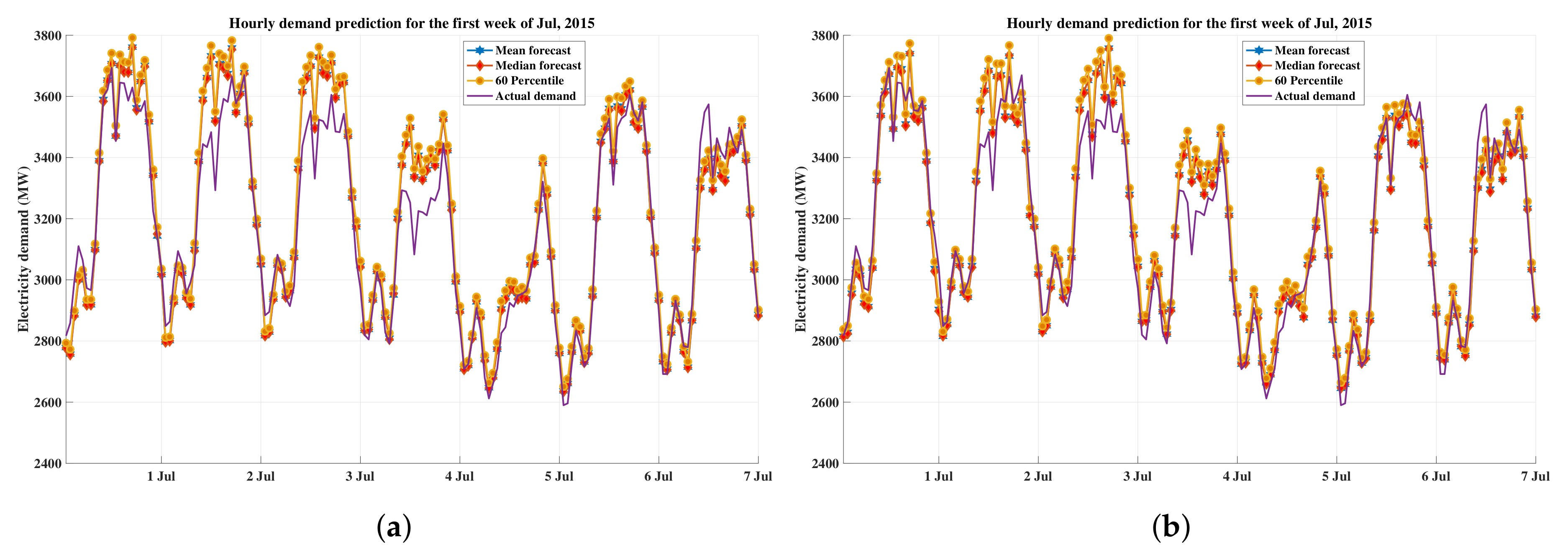
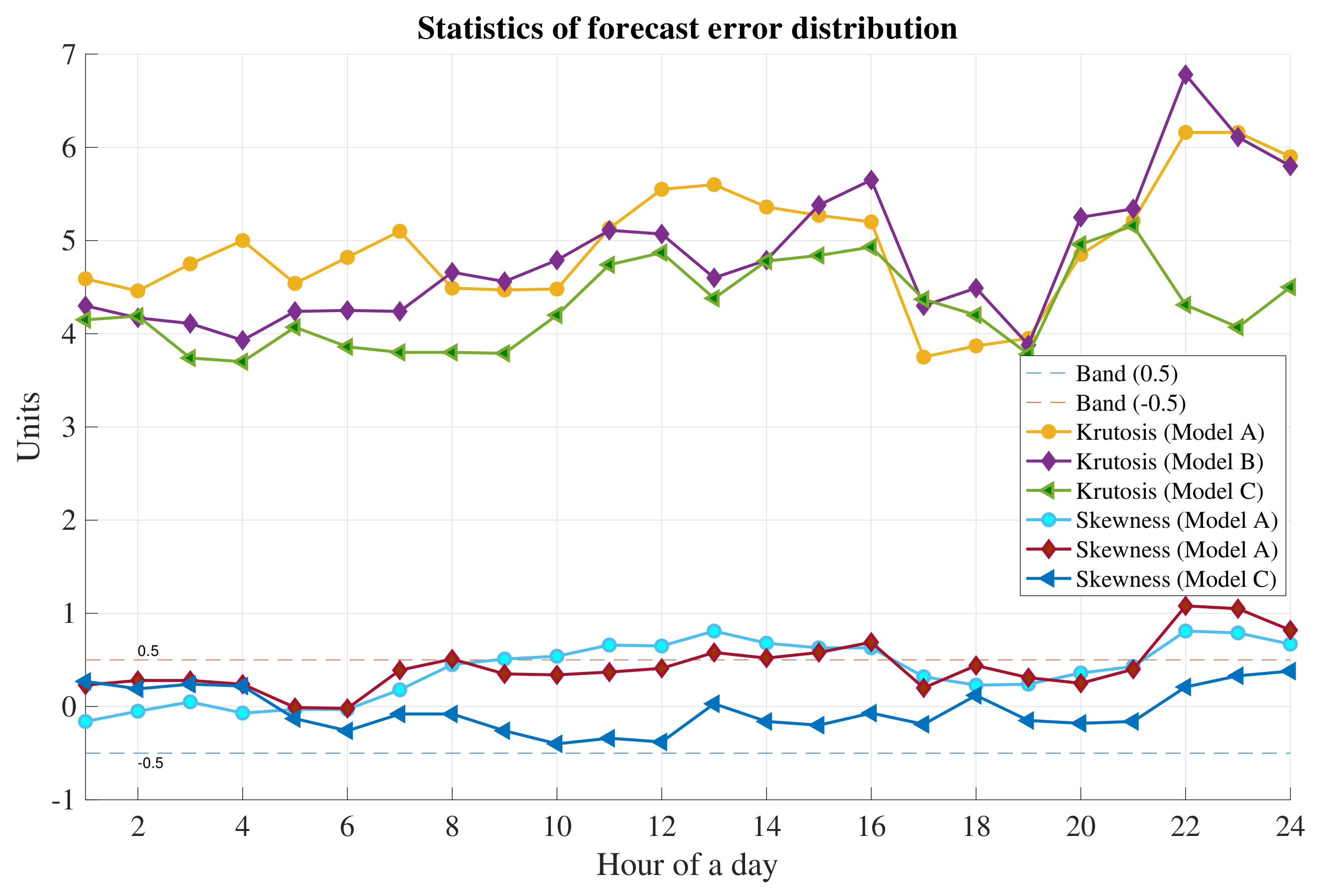
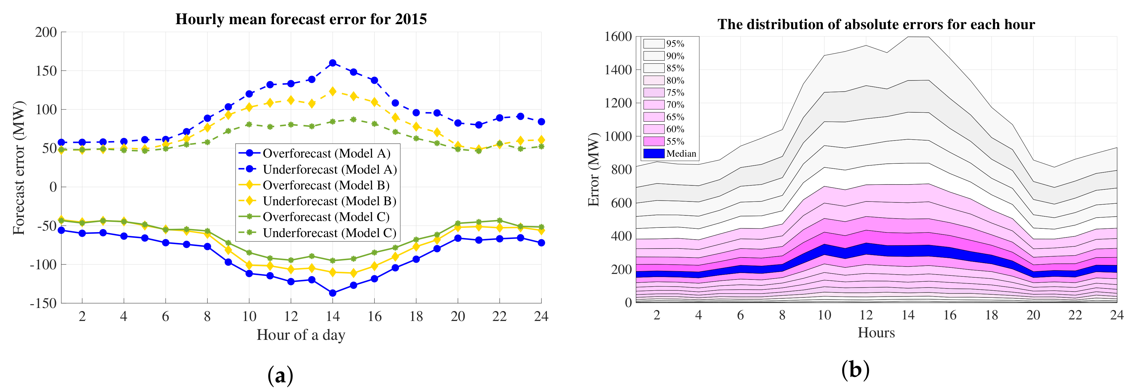
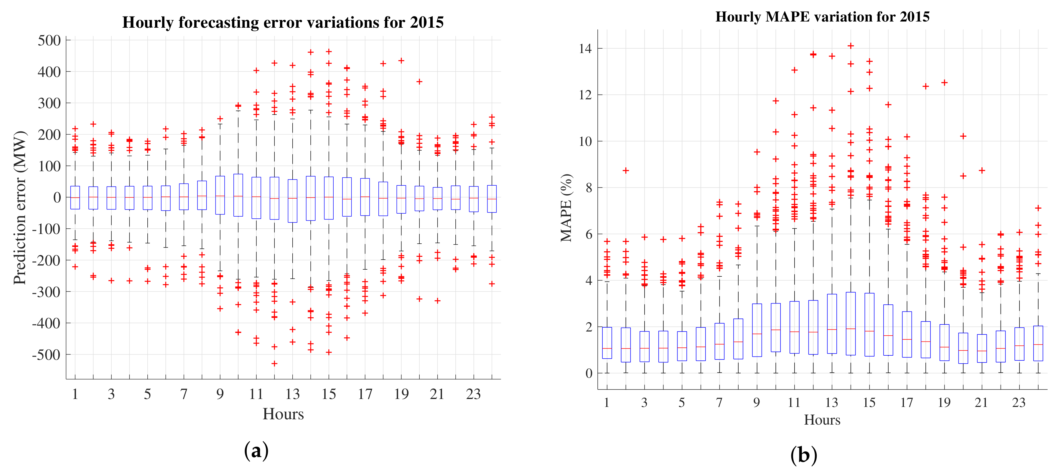
6. Results and Discussion

We have used three years of data up to 2015 from 2013 with no missing data. For training data, two years (730 days) of moving windows are used and predicted for the year 2015. The multiple equations modeled here are estimated for each hour with separate equations having their own co-variants. Therefore, for every hour of the day, they have a different weight of the parameter value.

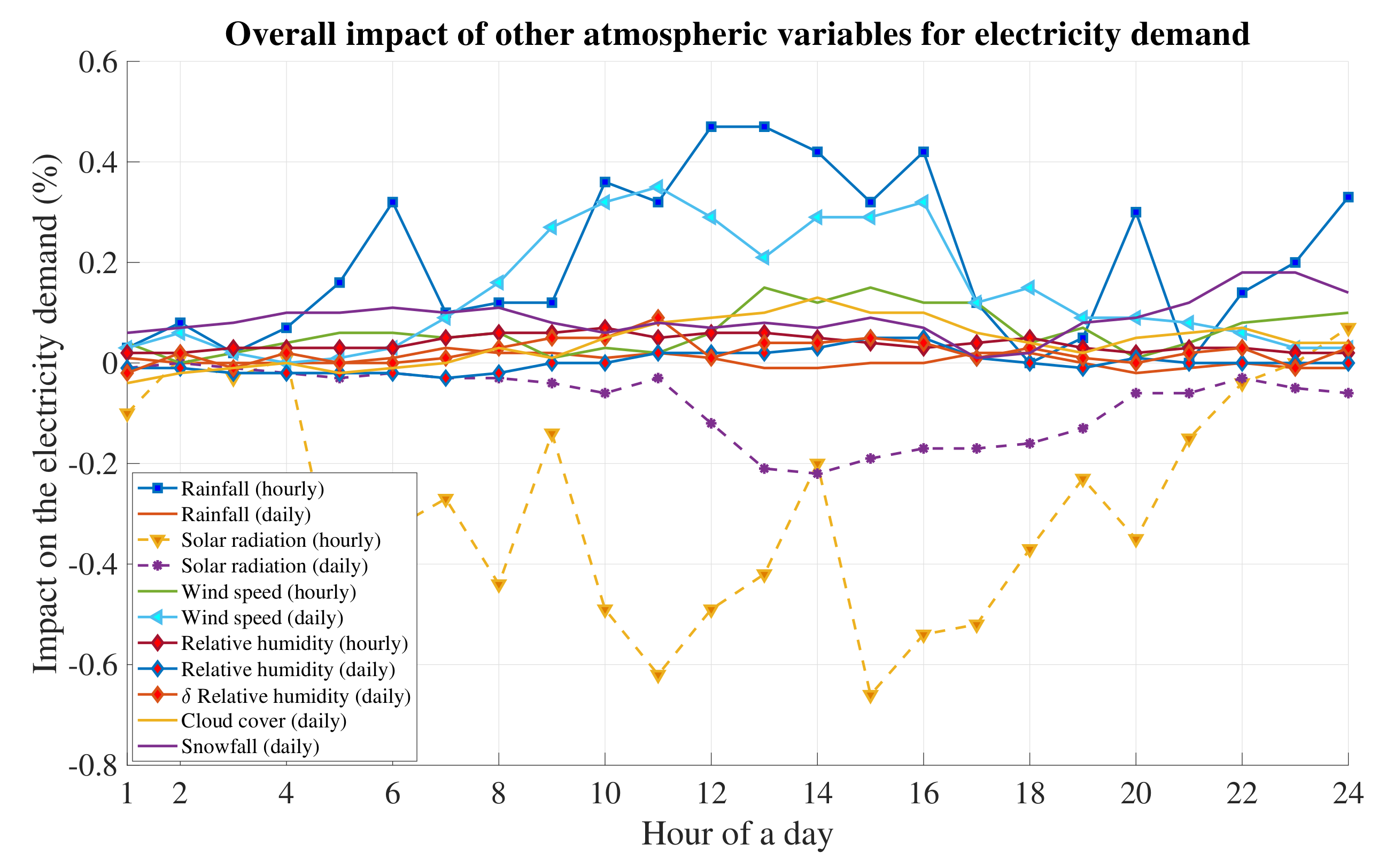
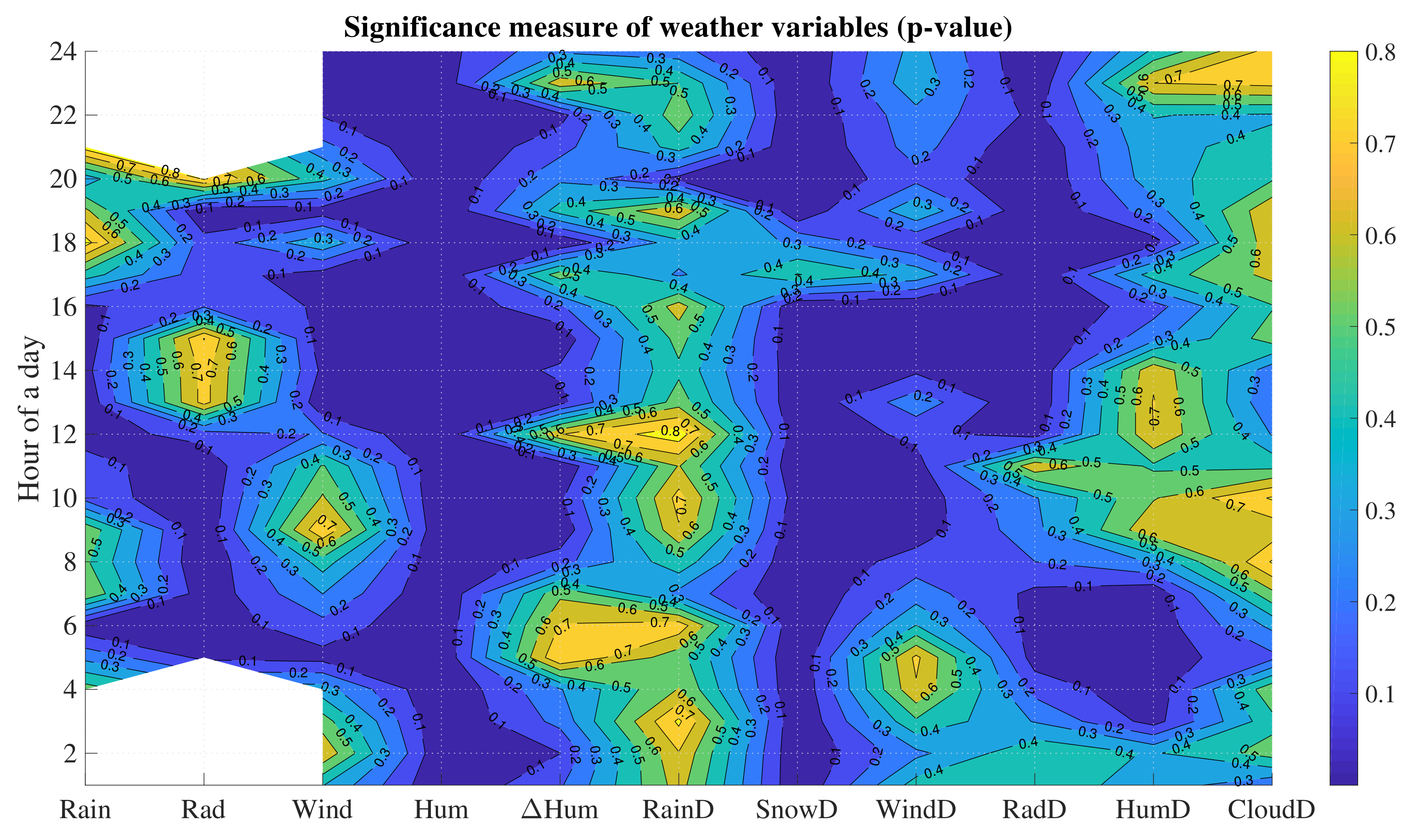
6.1. Atmospheric Variables

Since our motive is to find the atmospheric impact on electricity demand, their impacts vary according to the hour of the day. The estimated coefficients (only atmospheric variables are of interest to us) discussed for all the hours from Model C are plotted in Figure 5. Out of 26,280 samples, seven snowfall data and some cloud cover and humidity data were missing. Simple interpolation is used to fill up these missing data. At Hour 14, these variables show higher weights compared to other hours. The statistical and hypothesis testing of these weights is discussed in Section 6.4.

Figure 5 shows the overall impact of rainfall, solar radiation, wind speed, relative humidity, and cloud cover for all the hours. Rainfall during day hours (Hour 10–Hour 16) causes an increase of the cold environment, therefore showing the highest impact for the increment in electricity demand up to 0.5% (i.e., 18 MW for weekends, 18.4 MW for holidays and 20 MW for weekdays), followed by wind speed. However, sunlight (solar radiation) causes the environment to warm, and people use less heating appliances, which causes a decrease in demand during day hours. This is the reason why Hour 11 and Hour 15’s electricity demand is reduced by more than 0.6% (approximately 23 MW in aggregate) by solar radiation. From Hours 8 to 18, the electricity demand is significantly affected by wind speed, as the demand is increased to 0.38%. The correlation figure (Figure 3) indicates that cloud cover has the highest positive correlation with electricity demand, among these weather parameters. This is because cloud cover causes people to turn on lights, but the estimated parameter value for cloud cover shows up to a 0.16% increment only. Snowfall causes a slight increment during evening to morning hour, but humidity does not show any significant changes on electricity demand. In general, atmospheric sensitivities appear from Hour 5–Hour 22, mainly Hour 9–Hour 17. This result is comparable to a previous study’s result covering a business district of Tokyo Prefecture [36].

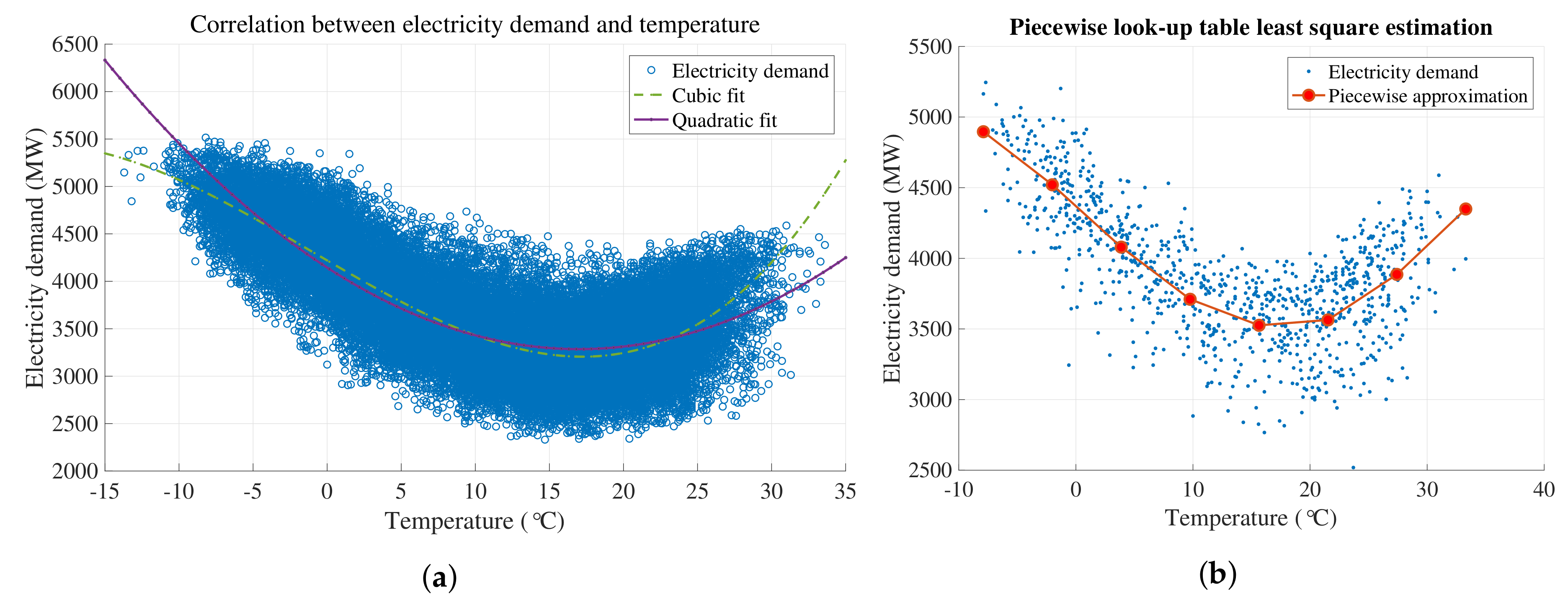
6.2. Temperature Variables

CDD and HDD terms are used to convert the non-linear relation of temperature to the linear relation by estimating the base temperature. However, still, square terms of CDD and HDD exist in the model. Therefore, the interpretation procedure of these terms and their impact on electricity demand are slightly different.

Table 3. Temperature coefficients’ analysis.

Temperature °C	Hour 1			Hour 14			Hour 19
	CDD_val	Deviation	$\mathit{\delta }\mathit{Demand}$	CDD_val	Deviation	$\mathit{\delta }\mathit{Demand}$	CDD_val	Deviation	$\mathit{\delta }\mathit{Demand}$
19.000	−5.3611	−0.0178	−1.7623	−3.0000	−0.0194	−1.9206	−1.1465	0.0068	0.6854
20.000	−4.3611	−0.0119	−1.1783	−2.0000	−0.0134	−1.3303	−0.1465	0.0165	1.6629
21.000	−3.3611	−0.0059	−0.5909	−1.0000	−0.0074	−0.7365	0.8535	0.0262	2.6498
22.000	−2.3611	0.0000	0.0000	0.0000	−0.0014	−0.1392	1.8535	0.0358	3.6463
23.000	−1.3611	0.0059	0.5944	1.0000	0.0046	0.4618	2.8535	0.0455	4.6525
24.000	−0.3611	0.0119	1.1924	2.0000	0.0106	1.0664	3.8535	0.0551	5.6684
25.000	0.6389	0.0178	1.7939	3.0000	0.0166	1.6746	4.8535	0.0648	6.6942
26.000	1.6389	0.0237	2.3990	4.0000	0.0226	2.2865	5.8535	0.0745	7.7299
27.000	2.6389	0.0296	3.0077	5.0000	0.0286	2.9021	6.8535	0.0841	8.7758
28.000	3.6389	0.0356	3.6200	6.0000	0.0346	3.5213	7.8535	0.0938	9.8317
29.000	4.6389	0.0415	4.2359	7.0000	0.0406	4.1443	8.8535	0.1034	10.8979
30.000	5.6389	0.0474	4.8555	8.0000	0.0466	4.7711	9.8535	0.1131	11.9745
31.000	6.6389	0.0533	5.4788	9.0000	0.0526	5.4016	10.8535	0.1228	13.0615
32.000	7.6389	0.0593	6.1058	10.0000	0.0586	6.0359	11.8535	0.1324	14.1591

illustrates the increase in electricity demand due to CDD for Hour 1, Hour 14 and Hour 19 based on the reference temperature. The second column explains the CDD values for the corresponding temperature in the first column. These CDD values are re-estimated from the partial derivative of $De{m}_d$ with respect to CDD, then solving the new CDD value (CDD_val), setting the equation equal to zero.

Since the CDD value cannot be negative, therefore the first five rows are neglected. During night time, for instance Hour 1, when the temperature increased from 25–26 °C, the demand is predicted to rise from 1.19–1.79%. Moreover, for the same temperature during Hour 19, electricity demand is predicted to increase from 6.69–7.72%. When the temperature reaches 32 °C, electricity demand is expected to be increased by 14.15% during peak hours of the evening because of more human activities in the evening time. However, for other hours, there is less than half the impact of temperature compared to Hour 19.

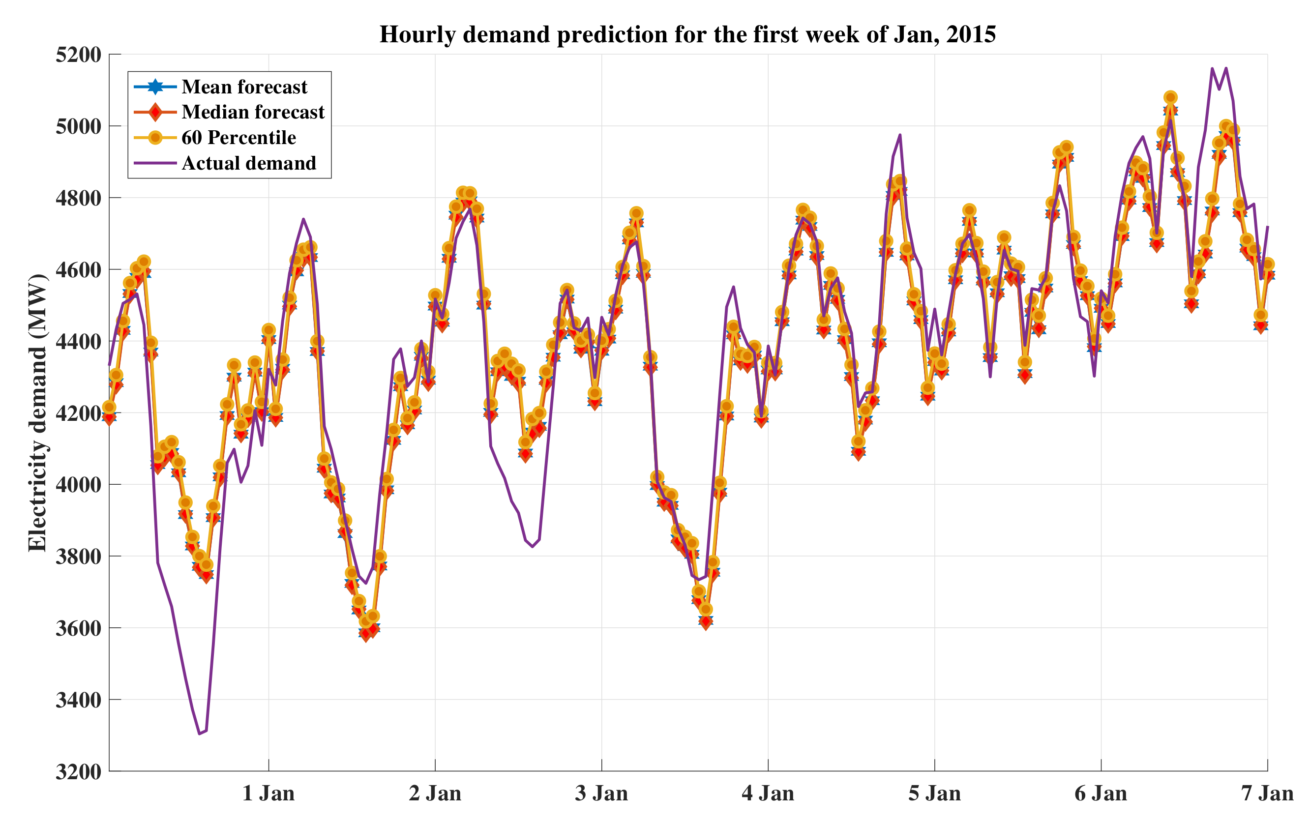
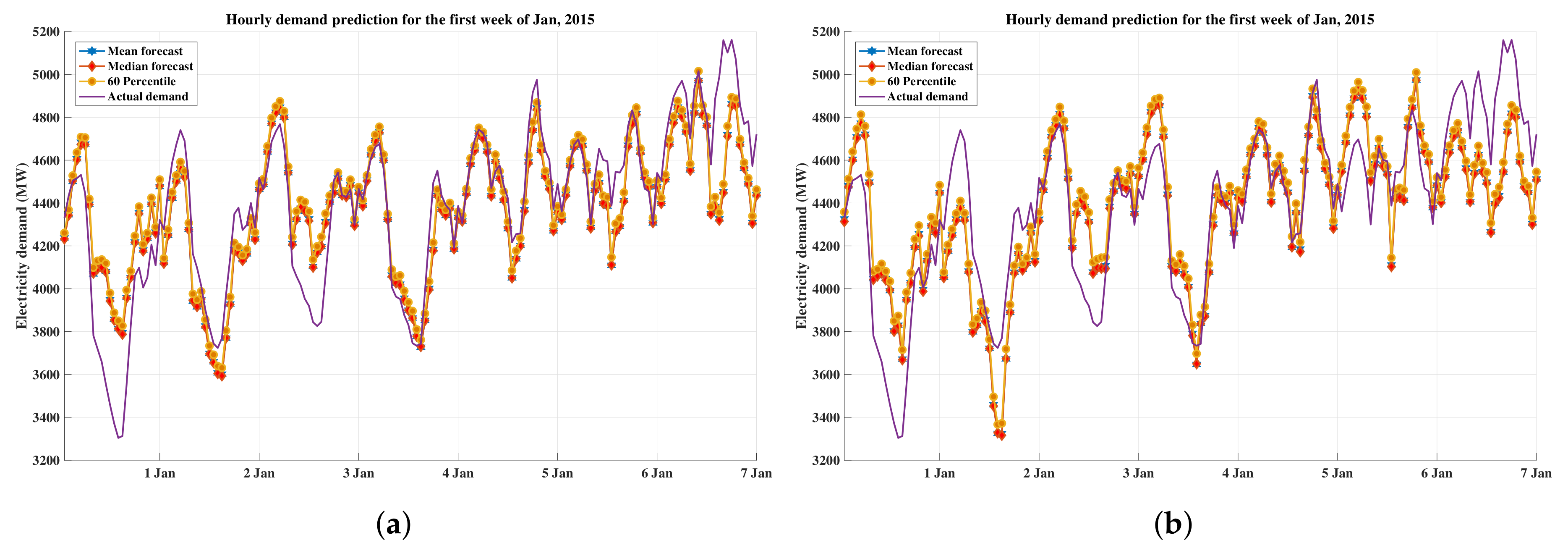
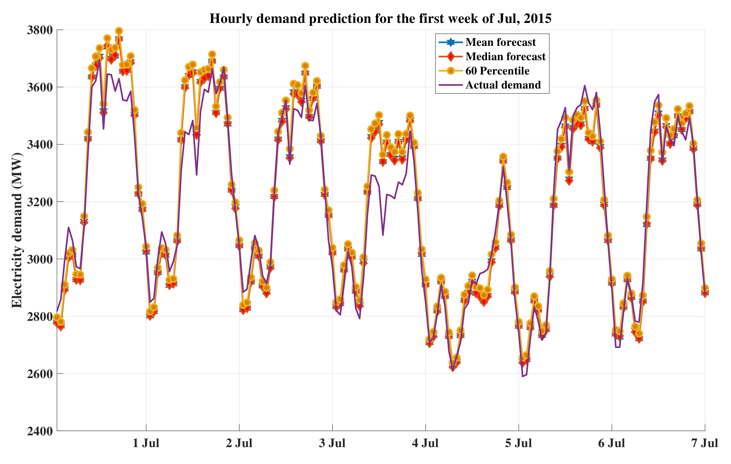
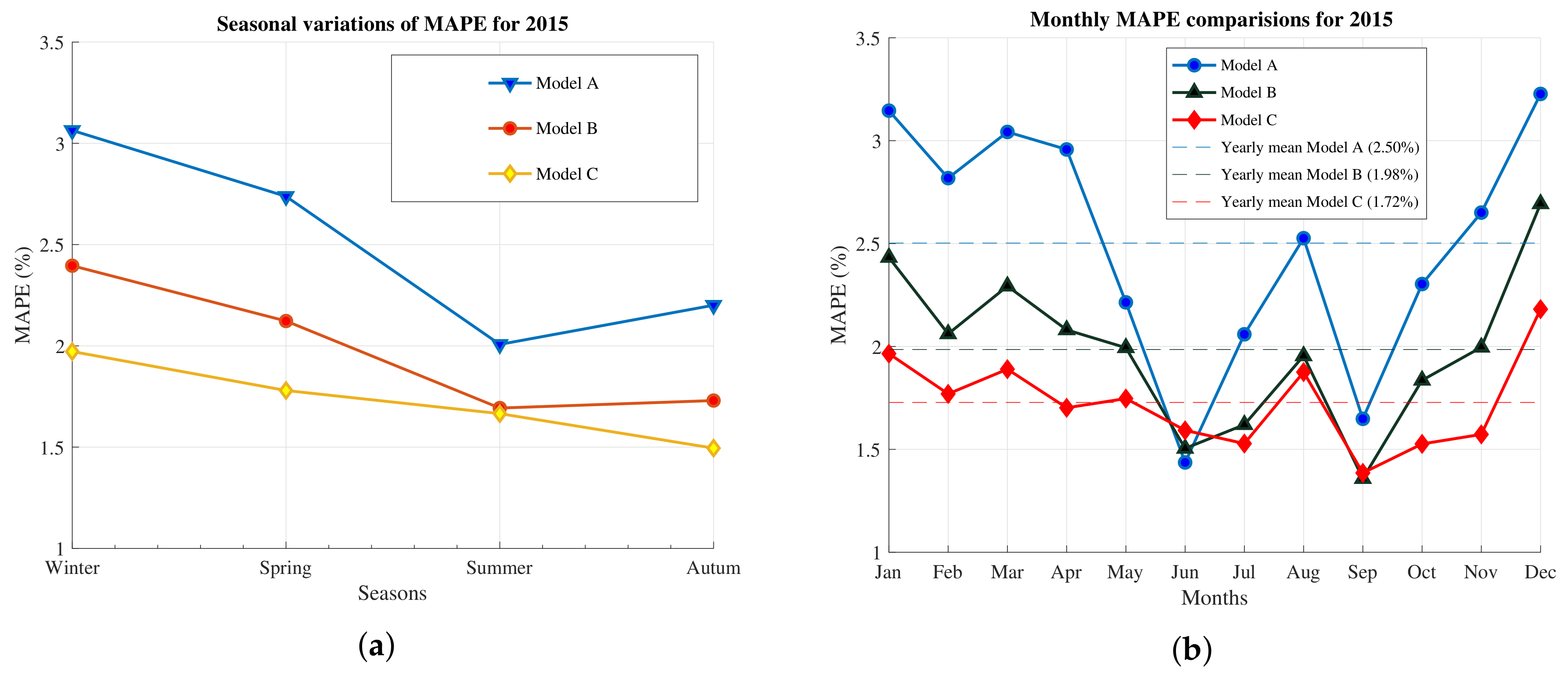
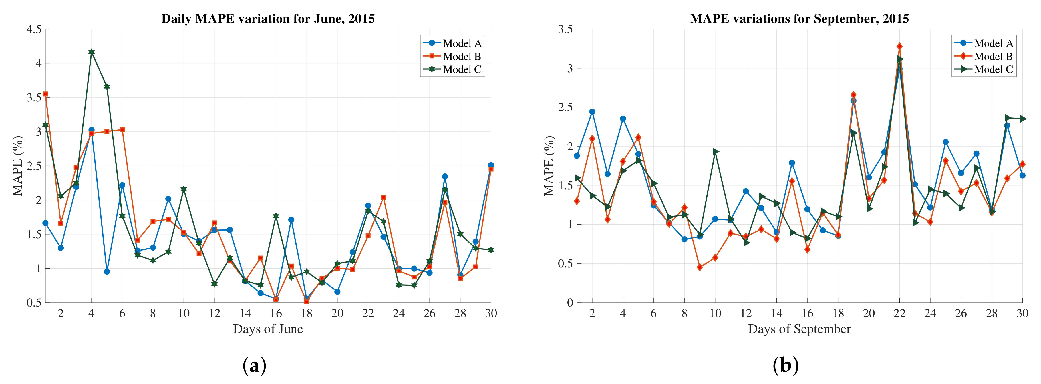
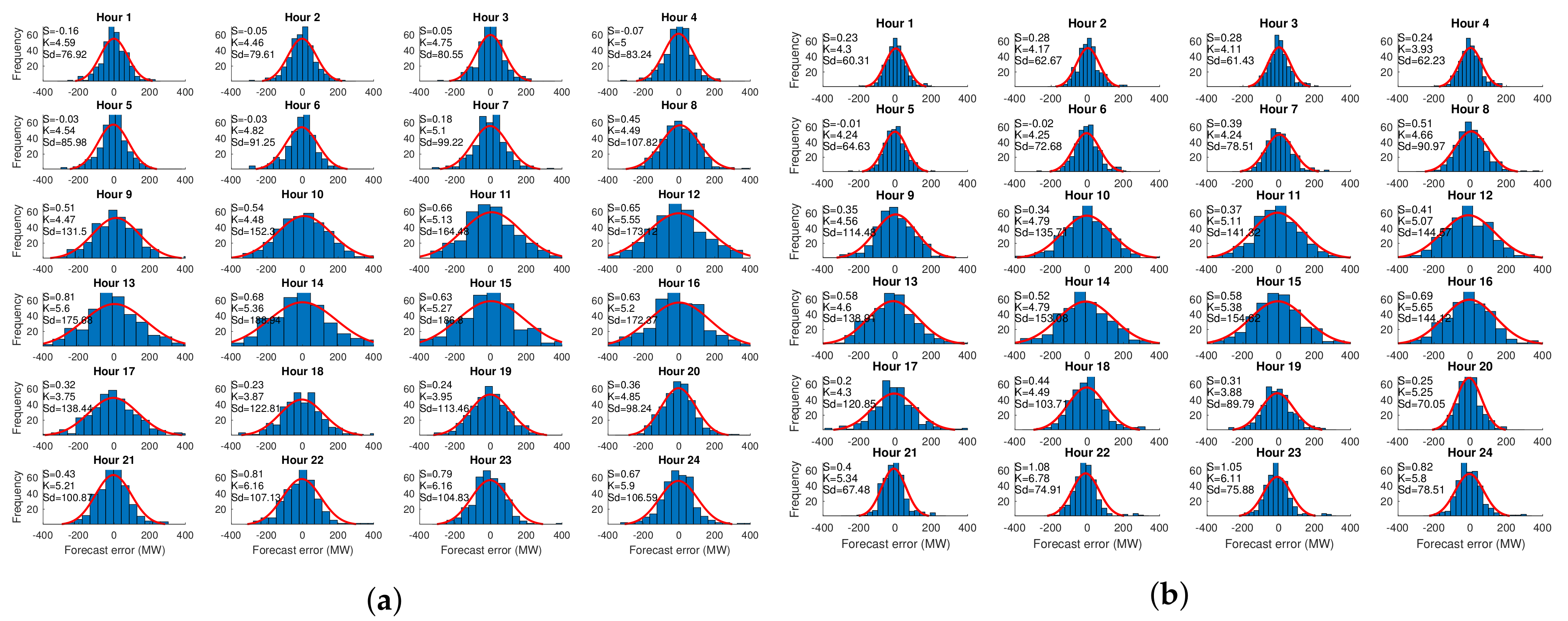
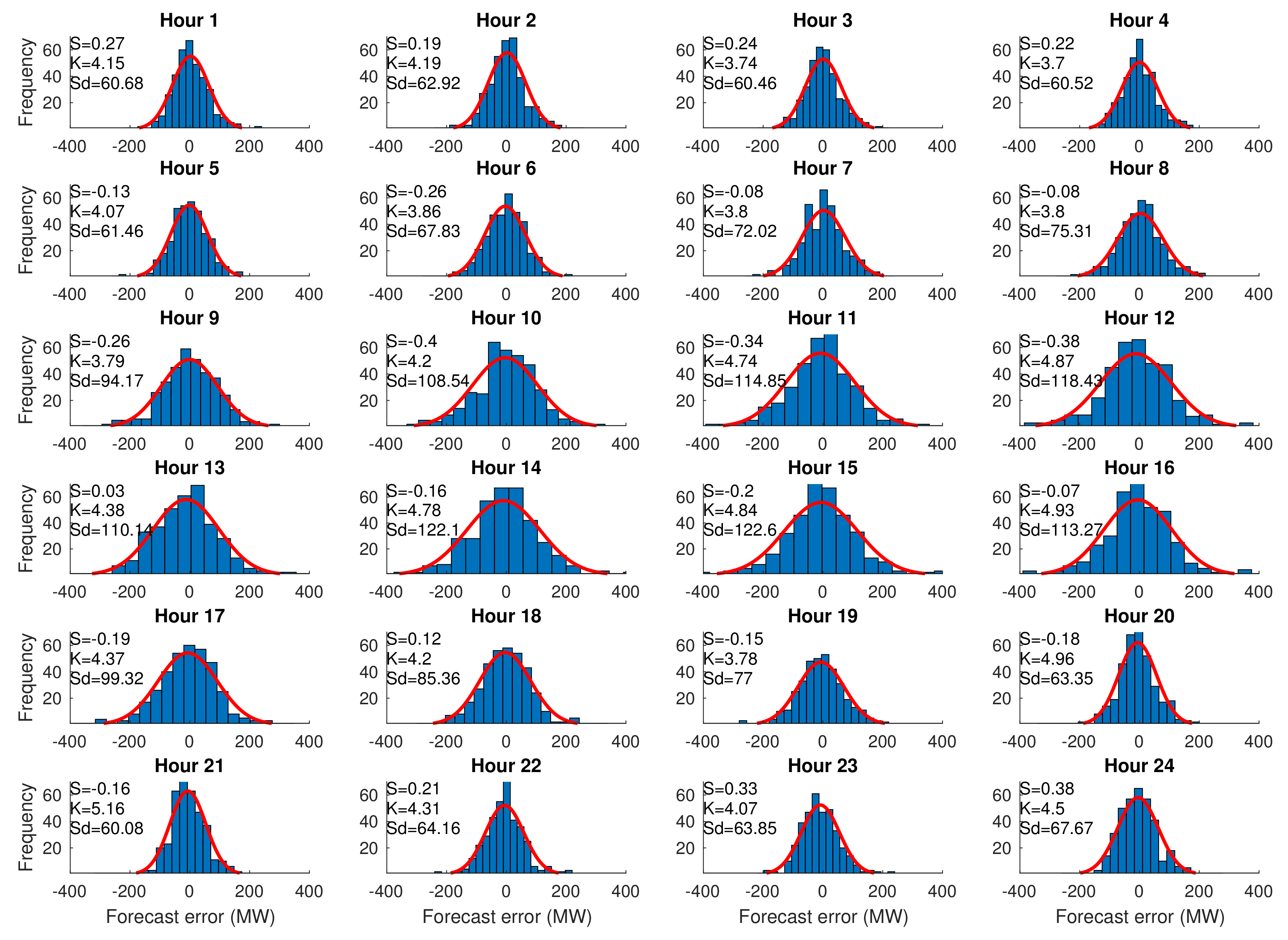
6.3. Performance Analysis

In Figure 6, electricity demand prediction by Model C is plotted for the first week of January 2015 and compared with the actual demand. The mean, median, and 60 percentile forecast values from the posterior distribution are implemented for prediction, which is the beauty of Bayesian estimation. Due to the New Year’s effects, forecasting performance is worse than other weeks. This week consists of a scheduled public holiday, unscheduled holidays, weekdays, and weekends. Therefore, it is worth discussing their effects on forecasting accuracy. The best MAPE performance for this week is 2.73% by Model C followed by Model B, while the worst performance is 4.25% (Model A). When the electricity demand for 1 January is predicted, the AR influence is clearly observed because the effect of previous days (high demand days) causes over-forecasting. Similarly, the electricity demand for 2 January is under-forecasted because of the lower demand of its previous day (1 January). As a normal Saturday demand, electricity demand is forecasted for 3 January, but actual demand is still lower than forecasted due to the New Year’s impact. Therefore, this week has a significant rise and fall of electricity demand.

Similarly, Figure 7a,b explains the hourly demand prediction by Model B, and Model A, respectively, for the same time period as Model C. The existence of higher forecast error caused by Model A, especially on 2 January, 4 January and 7 January, is minimized by model B. However, the predictive nature of all the models (Model A, Model B, and Model C) follows similar patterns, but comparatively, Model C is better.

In Figure 8, electricity demand prediction by Model C is plotted for the first week of July (summer season) 2015 and compared with actual demand. Electricity demand on 4 July (Saturday) is significantly over-forecasted. However, fluctuations in peaks are forecasted well. This week consists of one scheduled public holiday on 7 July (Tuesday), where both Model A, and Model B failed to predict the peak demand (Figure 9a,b). However, Model C predicted it very close to the actual demand. The best MAPE performance for this week is 1.69% by Model C, followed by Model A, while Model B is the worst with 1.96%.

Figure A1 and Figure A2 illustrate the prediction error distribution of each model for individual hours. As was our expectation, error variation during day hours is higher than other hours. Model A predicts the highest variation in error distribution of 188 at Hour 14. This variation in the same hour is reduced to 122 by Model C. The skewness and kurtosis plot in Figure 10 compares the error distribution statistics among the models for individual hours. A positive skewness value reflects a large number of positive errors, which means an under-forecasting of the electricity demand forecasting. Unlike Model A and Model B, Model C shows negative skewness during day hours, indicating the occurrence of over-forecast. Nevertheless, skewness values from Model C lie within the ±0.5 band, being equivalent to a normal distribution.

Similarly, kurtosis criteria are a measure of how prone a distribution with a value of three is to outliers, being equivalent to a normal distribution. A high kurtosis value can be interpreted as a failure to predict high electricity demand occurrence. Model C being closer to three compared to the other two models indicates that Model C is better. This can be seen more clearly in Figure 11a,b. Over-forecasting and under-forecasting characteristics of all three models are compared for all hours of a day. At Hour 14, Model A over-forecasts up to more than 155 MW followed by Model B, and Model C, respectively. Similarly, under-forecasting also occurs at the same Hour 14. However, the highest value for under-forecasting is less than 150 MW. Moreover, after Hour 20 until Hour 8, Model C can predict withing a ±50 MW forecast error, which is 1.2–1.4% MAPE in aggregate demand for these hours. Higher forecasting error has occurred during other hours (Hour 9–Hour 19), which is also explained in Figure 11b. The forecast distribution of absolute errors for each hour (Hour 9–Hour 19) is wider when most peaks occur.

This box plot in Figure 12a shows the hourly deviation of predicted demand from real electricity demand. Throughout the hours, the median value is zero, but during day hours, especially Hour 9–Hour 17, higher variations in the error occurred. As was our expectation, the over- and under-forecasting probabilities are approximately equally distributed. However, at Hour 10, there is a negligible probability for under-forecasting. Another important intuition from this box plot in Figure 12a is that forecasting error is randomly distributed with zero mean with some variance.

We have used the median value for the prediction of electricity demand because the median value minimizes the sum of absolute deviations. During simulations, the accuracy of electricity forecasting was measured by MAPE and the root mean square error (RMSE). For better accuracy, MAPE and the corresponding RMSE value should be low. However, only MAPE is presented in this paper for simplicity. Figure 12b indicates the box plot for accuracy measured in MAPE for each hour. The box plot can clearly explain the distribution of MAPE as a different percentile form. The MAPE value in our range (25th–75th percentile) is considered as an outlier in the box-plot and denoted by (+) in the plot. There are significant MAPE outliers throughout the hours that directly cause a higher mean MAPE value. The maximum MAPE is observed at morning Hour 9, afternoon Hour 14 and night Hour 23. This is because of the fluctuating electricity demand based on human activities during these periods.

Comparing the seasonal forecasting performance for all three models in Figure 13, Model A shows the worst MAPE value greater than 2% for all four seasons. However, for the same four seasons, Model C can forecast with less than 2% MAPE. Interestingly, the summer months from all the models show better forecasting performance. This is because the lower the demand, the lower the error probability and vice versa. This could be one reason why winter has a higher MAPE value than summer for all three models.

The hourly performances of Model A, Model B, and Model C are tabulated in the

Table A2. Hourly MAPE variation for various day types: working days including holidays (WDH), workings day not including holidays (WDNH), weekends including holidays (WEH), weekends not including holidays (WENH), holidays on working days (HWD), holidays on weekends (HWE).

Hour	Model	Sunday	Monday	Tuesday	Wednesday	Thursday	Friday	Saturday	WDH	WDNH	WEH	WENH	HWD	HWE	Holiday	NH
1	Model A	1.6726	1.7407	1.7456	1.8309	1.5394	1.4631	1.4922	1.6639	0.7753	1.5824	1.6213	1.9812	0.8121	1.7474	1.6325
	Model B	1.1504	1.4382	1.2741	1.4257	1.2117	1.4709	1.2896	1.3642	0.7606	1.2200	1.2131	1.4685	1.3576	1.4463	1.3136
	Model C	1.1919	1.4357	1.3395	1.4745	1.1992	1.5799	1.2373	1.4057	0.8193	1.1919	1.2274	1.6611	0.9614	1.5212	1.3382
2	Model A	1.8561	1.7041	1.6715	1.8159	1.5774	1.5581	1.5430	1.6654	0.8006	1.6996	1.7156	2.1112	1.3818	1.9653	1.6535
	Model B	1.2177	1.4480	1.1882	1.4230	1.2913	1.5818	1.4109	1.3865	0.7887	1.3143	1.3056	1.3492	1.4865	1.3767	1.3648
	Model C	1.2970	1.4602	1.1697	1.4413	1.2717	1.6941	1.3749	1.4074	0.8426	1.2970	1.3407	1.5256	1.2430	1.4691	1.3806
3	Model A	1.8299	1.6551	1.7280	1.8782	1.5712	1.3902	1.3610	1.6445	0.6908	1.5954	1.6039	2.2782	1.4283	2.1082	1.5952
	Model B	1.2882	1.3785	1.1462	1.4060	1.1784	1.3799	1.3110	1.2978	0.7097	1.2996	1.3006	1.2319	1.2804	1.2416	1.3021
	Model C	1.3373	1.3129	1.1836	1.3597	1.1587	1.4631	1.3420	1.2956	0.7436	1.3373	1.3548	1.3017	1.0399	1.2494	1.3121
4	Model A	1.7652	1.6379	1.8458	1.8160	1.6098	1.3923	1.3475	1.6604	0.6981	1.5563	1.5657	2.2030	1.3701	2.0364	1.6007
	Model B	1.1658	1.2604	1.1607	1.3288	1.2750	1.4508	1.3543	1.2952	0.7567	1.2600	1.2595	1.1060	1.2704	1.1389	1.2958
	Model C	1.1385	1.2825	1.1582	1.3299	1.1545	1.4228	1.3618	1.2696	0.7364	1.1385	1.2624	1.0859	1.0082	1.0704	1.2779
5	Model A	1.8329	1.6645	1.9004	1.9173	1.5649	1.5715	1.3441	1.7237	0.7901	1.5885	1.5814	2.3748	1.7288	2.2456	1.6435
	Model B	1.3387	1.3066	1.3126	1.3861	1.2598	1.4386	1.3605	1.3407	0.7509	1.3496	1.3297	1.4274	1.7425	1.4904	1.3322
	Model C	1.3420	1.3241	1.2364	1.4013	1.1265	1.4575	1.2308	1.3092	0.7773	1.3420	1.2897	1.3027	1.2207	1.2863	1.3033
6	Model A	1.9198	1.9072	2.0596	1.9769	1.5467	1.5389	1.6301	1.8059	0.7545	1.7750	1.8003	2.5605	1.2725	2.3029	1.7591
	Model B	1.6503	1.5450	1.6708	1.5754	1.1965	1.4065	1.5892	1.4789	0.7142	1.6197	1.5820	1.6762	2.3669	1.8144	1.4965
	Model C	1.6451	1.5607	1.5380	1.5917	1.1067	1.3907	1.4814	1.4376	0.7524	1.6451	1.5595	1.4951	1.6376	1.5236	1.4687
7	Model A	2.0690	2.1267	2.2502	2.2338	1.8833	1.6164	1.9340	2.0221	0.7776	2.0015	2.0574	2.9955	0.8951	2.5754	1.9747
	Model B	1.7640	1.7209	1.7645	1.6313	1.4183	1.4893	2.0553	1.6049	0.7315	1.9097	1.9323	2.4035	1.4605	2.2149	1.6527
	Model C	1.6466	1.7467	1.5595	1.5090	1.2270	1.4631	1.7972	1.5011	0.7673	1.6466	1.7573	2.0983	1.0206	1.8828	1.5397
8	Model A	2.2325	2.3071	2.2233	2.5286	2.4832	2.1212	2.4363	2.3327	1.0441	2.3344	2.3803	3.4155	1.4263	3.0177	2.2833
	Model B	1.8220	1.8314	1.9199	1.9725	1.8258	1.7969	2.5240	1.8693	0.8740	2.1730	2.1622	2.8535	2.3874	2.7603	1.8966
	Model C	1.5913	1.5995	1.5147	1.6427	1.4574	1.5827	2.1622	1.5594	0.8269	1.5913	1.8738	2.2654	1.9355	2.1994	1.6091
9	Model A	2.6461	2.4470	2.7248	2.7950	2.8503	2.4008	3.1912	2.6436	1.1834	2.9187	2.8304	4.3900	4.6659	4.4452	2.5959
	Model B	2.1982	2.0883	2.2785	2.2846	2.4666	2.1374	3.1797	2.2511	1.0574	2.6890	2.5874	3.8711	4.6995	4.0367	2.2544
	Model C	1.9150	1.7530	1.7447	1.9969	1.9034	1.8084	2.8321	1.8413	0.9390	1.9150	2.2789	3.4363	4.2477	3.5986	1.8751
10	Model A	2.9442	2.6022	3.2205	3.0529	3.1272	2.6851	3.6793	2.9376	1.3814	3.3117	3.1540	4.5038	6.4350	4.8900	2.9090
	Model B	2.4234	2.3307	2.6872	2.3936	2.7461	2.7183	3.5322	2.5752	1.4121	2.9778	2.8153	4.0603	6.1947	4.4871	2.5583
	Model C	2.1795	2.0551	2.1036	1.9529	2.1555	2.0213	3.0005	2.0577	1.1097	2.1795	2.4479	3.4744	5.4029	3.8601	2.0883
11	Model A	3.2398	2.6796	3.3393	3.2835	3.2169	2.9312	3.9262	3.0901	1.5203	3.5830	3.3519	4.4814	8.1586	5.2168	3.0849
	Model B	2.5062	2.3502	2.7765	2.5841	2.6018	2.9451	3.6375	2.6516	1.5283	3.0718	2.8516	4.2028	7.4327	4.8488	2.6184
	Model C	2.3283	1.9570	1.9768	2.2351	2.1442	2.2174	3.0316	2.1061	1.2075	2.3283	2.4878	3.2880	6.4853	3.9274	2.1478
12	Model A	3.1075	2.8537	3.4770	3.4629	3.4499	3.1050	3.9691	3.2697	1.6391	3.5383	3.3037	4.9317	8.1837	5.5821	3.1824
	Model B	2.5170	2.5425	2.9768	2.7074	2.8006	3.0701	3.5237	2.8195	1.6153	3.0203	2.8234	4.9172	6.9190	5.3175	2.6972
	Model C	2.3383	2.1527	2.0263	2.2816	2.2020	2.3525	2.9905	2.2030	1.2876	2.3383	2.4675	3.6795	6.5631	4.2562	2.1932
13	Model A	3.3161	2.8978	4.0335	3.7530	3.3656	3.5846	3.8910	3.5269	1.8386	3.6036	3.3948	4.6860	7.7364	5.2961	3.4198
	Model B	2.4320	2.6308	3.2304	2.9576	2.7321	3.1860	3.3674	2.9474	1.6902	2.8997	2.7367	3.8506	6.1283	4.3061	2.8323
	Model C	2.2623	2.1179	2.1186	2.3961	2.2355	2.5430	2.7583	2.2822	1.3922	2.2623	2.3490	3.0000	5.7045	3.5409	2.2593
14	Model A	3.6238	3.0059	4.0271	3.8494	3.3133	3.9163	4.3122	3.6224	1.9851	3.9680	3.7592	5.5966	8.1018	6.0977	3.5452
	Model B	2.5357	2.6686	3.3307	3.2034	2.7270	3.4654	3.7935	3.0790	1.8339	3.1646	2.9757	4.8298	6.9040	5.2447	2.9449
	Model C	2.2401	2.2966	2.0473	2.6013	2.1359	2.5819	3.0670	2.3326	1.3972	2.2401	2.4697	3.7217	6.2939	4.2362	2.2902
15	Model A	3.6812	3.0742	3.9871	3.7488	3.0118	3.9572	4.2087	3.5558	2.0035	3.9449	3.7478	5.2494	7.8475	5.7690	3.5105
	Model B	2.7848	2.6771	3.1999	3.3373	2.5674	3.2893	3.4836	3.0142	1.7151	3.1342	2.9288	4.9817	7.2022	5.4258	2.8723
	Model C	2.3425	2.2175	2.2240	2.4928	2.1483	2.6142	2.9446	2.3394	1.3864	2.3425	2.4668	4.1316	6.1436	4.5340	2.2705
16	Model A	3.5173	3.0099	3.5821	3.5607	2.7995	3.2589	3.8668	3.2422	1.6404	3.6920	3.6108	4.8270	5.2998	4.9216	3.2550
	Model B	2.7110	2.6691	2.7547	3.0173	2.3450	2.8460	3.2405	2.7264	1.4517	2.9758	2.8676	4.1300	5.1174	4.3275	2.6838
	Model C	2.2337	2.1280	2.0626	2.3022	1.9723	2.1713	2.6555	2.1273	1.1495	2.2337	2.3272	3.4206	4.7688	3.6903	2.1090
17	Model A	2.8113	2.2691	2.6527	2.8911	2.4075	2.5460	3.7121	2.5533	1.2941	3.2617	3.1543	3.3655	5.3881	3.7700	2.6801
	Model B	2.3903	2.2728	2.0630	2.4652	1.9515	2.1243	3.0331	2.1754	1.1075	2.7117	2.6350	3.1321	4.2301	3.3517	2.2523
	Model C	2.1376	1.9282	1.6517	1.8570	1.8850	1.7124	2.4634	1.8069	0.9375	2.1376	2.2313	2.5008	3.6711	2.7349	1.8899
18	Model A	2.2690	2.1932	2.2601	2.4965	2.2489	2.2088	3.0329	2.2815	1.1026	2.6509	2.6016	3.4705	3.6273	3.5019	2.3047
	Model B	1.8041	2.0382	1.7465	2.0586	1.7992	1.8877	2.4489	1.9061	0.9407	2.1265	2.0982	2.6811	2.6862	2.6822	1.9161
	Model C	1.8099	1.6286	1.3981	1.7202	1.7559	1.5168	1.8188	1.6039	0.7631	1.8099	1.7890	2.0452	2.3158	2.0993	1.6323
19	Model A	1.9400	2.1032	2.4597	1.7876	2.0171	2.0373	2.6626	2.0810	1.0018	2.3013	2.2479	3.1036	3.3588	3.1546	2.0693
	Model B	1.5986	1.9853	1.5508	1.5214	1.5875	1.7703	2.1094	1.6831	0.8720	1.8540	1.8295	2.9165	2.3402	2.8012	1.6528
	Model C	1.5358	1.7506	1.3152	1.1828	1.6486	1.3373	1.6731	1.4469	0.6953	1.5358	1.5810	2.3915	2.0686	2.3269	1.4310
20	Model A	1.7961	1.8596	1.7109	1.6868	1.8195	1.6626	2.3081	1.7479	0.8015	2.0521	1.9965	2.8977	3.1537	2.9489	1.7528
	Model B	1.3819	1.3910	0.9991	1.2920	1.2984	1.1858	1.6894	1.2333	0.5791	1.5357	1.5211	2.4375	1.8249	2.3150	1.2464
	Model C	1.3681	1.2429	0.9897	1.2038	1.2219	1.0033	1.4228	1.1323	0.5094	1.3681	1.3759	2.1167	1.7822	2.0498	1.1456
21	Model A	1.9851	1.8714	1.9007	1.7697	1.8257	1.7998	2.1877	1.8334	0.8843	2.0864	2.0404	2.9103	2.9981	2.9278	1.8303
	Model B	1.4202	1.4070	1.0795	1.1981	1.2286	1.1109	1.6524	1.2048	0.5500	1.5363	1.5231	2.2684	1.7980	2.1743	1.2350
	Model C	1.4664	1.2926	0.9844	1.0369	1.2318	1.0341	1.3425	1.1159	0.5441	1.4664	1.3868	2.1136	1.7543	2.0417	1.1364
22	Model A	2.1472	2.0246	1.9386	2.0494	1.8935	1.8998	2.1253	1.9612	0.9233	2.1363	2.0900	2.8940	3.0530	2.9258	1.9436
	Model B	1.4406	1.4008	1.3538	1.4628	1.3684	1.3452	1.6044	1.3862	0.6642	1.5225	1.5329	2.3268	1.3174	2.1249	1.3735
	Model C	1.4462	1.4146	1.2637	1.2127	1.3508	1.1255	1.3280	1.2734	0.6027	1.4462	1.3866	2.0830	1.3962	1.9457	1.2590
23	Model A	2.2922	1.9065	2.1283	2.2634	2.0251	2.0859	2.0248	2.0819	1.0168	2.1585	2.1233	2.6635	2.8549	2.7018	2.0595
	Model B	1.5580	1.5780	1.4537	1.5983	1.6215	1.5366	1.3977	1.5576	0.7889	1.4779	1.4828	1.7395	1.3809	1.6678	1.5253
	Model C	1.4426	1.4823	1.3921	1.4256	1.5368	1.4081	1.2703	1.4490	0.7731	1.4426	1.3404	1.5004	1.6744	1.5352	1.4146
24	Model A	2.2812	1.8947	2.3251	2.3162	1.9561	2.3125	1.9756	2.1609	1.1198	2.1284	2.0778	2.1986	3.1313	2.3852	2.1339
	Model B	1.7227	1.5818	1.6329	1.5357	1.8184	1.5679	1.5059	1.6273	0.8113	1.6143	1.6001	1.6980	1.8959	1.7376	1.6158
	Model C	1.6399	1.4829	1.4895	1.3902	1.5656	1.4349	1.3684	1.4726	0.7713	1.6399	1.4723	1.5999	2.1355	1.7070	1.4653

. The first row of the table contains the description of each column such as Column 1–7: hours, model types, and days of the week. Column 8–15 contain the MAPE values of working days including holidays (WDH), workings day not including holidays (WDNH), weekends including holidays (WEH), weekends not including holidays (WENH), holidays on working days (HWD), holidays on weekends (HWE), only holidays, and non-holidays, respectively. For each column, we are selecting the largest 20 (randomly chosen number) MAPE values (bold and italic) and smallest 20 MAPE values (bold) to compare the hourly performance of individual models.

In general, the performances of the three models for all days from the evening at Hour 19 until the morning at Hour 7 in the Table A2 show that 99% of the smallest MAPE values are within these periods. Similarly, more than 99% of the largest MAPE values occur during morning Hour 8 to evening Hour 18. This is because of human activities during day hours. Model A is 48.3%; Model B is 38.7%, responsible for the higher MAPE; whereas Model C is much less (13%) responsible for the higher MAPE. However, the important question is: Which model plays a significant role in the minimization of MAPE? Model C has the highest percentage (53.7%) having minimum MAPE followed by Model B (40.7%), and the lowest is Model A with 5.6%.

From morning Hour 9 to afternoon Hour 17, Model C can forecast with the best MAPE value (100%) compared to the other models. However, for 1 a.m. to 4 a.m., Model B can forecast with 60% of the best MAPE values. Getting smaller MAPE values during working hours of the day is very challenging for researchers. This is because of unpredictable human activities and weather variations. Therefore, during the peaks and fluctuating hours, Model C can be used for better forecasting accuracy. In Hokkaido, peak demand is during Hour 17, and for this time period as well, Model C performs very well. There is very less possibility of getting higher MAPE values from Model C compared to Model B and Model A.

Figure 13b compares the performance of Model C with Model B and Model A, based on the accuracy of their forecasting ability. Throughout the months of 2015, the accuracy of Model C is better than the other two models. However, unlike our expectation, the accuracies of Model A and Model B are superior in June and September, respectively. Nevertheless, the difference between the accuracies is relatively low (0.005% MAPE). The one reason behind this result is the dramatic change in the weather variables (Figure 15a,b). In June, Model B and Model C have very poor performance especially on 4, 5, 10 and 16 June; see Figure 14a. On 5 June, the performance of Model C is 3.6-times worse than Model A. Therefore, a strong reason behind the poor performance of Model B and Model C is the fluctuation of the weather variables, especially temperature (because both Models B and C perform poorly). Figure 15a justifies the reason. On June 2015, except the first week, there was normal variation of temperature with a mean of 16.70%. However, the temperature on 5 June 2015 dramatically decreases to the minimum level. This sudden variation in temperature forces the poor forecasting performance of both Models B and C.

Similarly, in September 2015, unlike our expectations, only Model B has very competitive performance with Model C. Nevertheless, the difference in accuracy is negligible. Since Model C includes rainfall, snowfall, solar radiation, wind, humidity, and cloud cover, we can assume that there must be some unpredictable variation in these variables. Figure 14b shows that especially for 10 and 30 September 2015, the forecasting performance of Model C is poor. This is because on 10 September 2015, wind speed unexpectedly rose to a peak. The increased value of cloud cover on the same day also supports this volatility (Figure 15b). Therefore, such unexpected variation in weather variables causes the forecasting performance to be always challenging.

The overall measure of forecasting accuracy in different MAPE ranges is reported in

Table 4. Measures of the forecasting accuracy for Models A, B, and C.

	Model Types	Overall MAPE (%)	Maximum MAPE (%)	MAPE ≤ 2%	MAPE > 2%	MAPE ≥ 5%	MAPE ≥ 10%	MAPE ≥ 15%	Observations
Overall	Model A	2.43	19.32	53.5	46.5	11.56	1.09	0.19	8760
	Model B	1.98	15.41	62.49	37.51	6.97	0.53	0.01
	Model C	1.72	14.06	67.93	32.07	4.05	0.23	0
Working days	Model A	1.15	19.04	54.78	45.22	9.71	0.69	0.12	5784
	Model B	1.03	13.8	64.93	35.07	5.53	0.32	0
	Model C	0.90	13.35	70.35	29.65	2.71	0.172	0
Weekends	Model A	2.49	11.93	52.87	47.13	12.66	0.92	0	2376
	Model B	2.03	11.75	60.56	39.44	7.82	0.21	0
	Model C	1.81	9.2746	66.28	33.71	5.57	0	0
Holidays	Model A	3.52	19.33	43.5	56.5	25	5.66	1.66	600
	Model B	2.93	15.42	46.5	53.5	17.5	3.83	0.16
	Model C	2.51	14.06	51.17	48.83	11.33	1.66	0

, in which Models A, B, and C are compared. Tabulated values in the third column express the overall MAPE for 2015. Comparing all the models, the most significant MAPEs are obtained from Model C for all cases. More specifically, the introduction of all weather variables in Model C reduces the high MAPE values (MAPE ≥ 5%) by one-fourth on working days and at least by half on other days. The overall MAPE performances of Models A, B, and C are 2.43%, 1.98%, 1.72% respectively. Therefore, the performance is improved by 18.5%, if we include temperature with historical electricity demand data. Similarly, Model C can improve forecasting accuracy by 13.4%, by including other atmospheric variables.

6.4. Hypothesis Testing

We test the statistical significance for two aspects: statistical significance of other atmospheric variables and statistical significance for accuracy improvement by Model C. Since these atmospheric variables are added in Model C, the statistical significance of the estimated weights is tested (Figure 16). After Hour 20, there is no solar radiation data available until morning Hour 5; therefore, a void contour graph exist during those hours. The estimated weight of relative humidity (hourly) is significant for all hours, whereas daily rainfall and daily cloud cover are strongly not significant. Other variables such as wind speed (hourly and daily), solar radiation (hourly and daily) and hourly rainfall are fairly significant for some hours.

To analyze the improvement in accuracy by Model C, a one-sided z-test for 99% confidence is used for all individual hours. We determine whether the accuracy of any hour is significantly improved by adding atmospheric variables (Model C) compared to the accuracy of other models (without atmospheric variables) or not. The null hypothesis states that there is no significant difference in the models’ performance tested at the 0.01 level against the alternative hypothesis. Testing the accuracy with respect to Model A, the test result shows that Model C has a significant improvement of the accuracy for all the hours of a day. However, testing the accuracy of Model C with respect to Model B, we cannot obtain sufficient evidence to reject the null hypothesis for Hours 1–6. i.e., the improvement of the accuracy by Model C during Hours 1–6 is statistically not significant. However, the improvement of the accuracy for the rest of the hours is statistically significant.

6.5. Computation Time

The computational time of the forecast model is important for utilities. If online training is used, where electricity demand observations from each day are added to the training dataset for model retraining, computational time plays a crucial role. When conducting an electricity demand forecast for 24 h ahead, the computational time depends on the length of the moving window, the number of predictors used and, most importantly, the selected forecasting technique. In this study, the computational time to forecast for 24 h was approximately 0.20 min for the OLS technique (for all three models). However, for the Bayesian technique, it was significantly higher than the OLS technique. The computational times to forecast for the next 24 h of Model A, Model B, and Model C were recorded as 3.77 min, 5.682 min and 7.919 min, respectively. The simulation was conducted on an Intel Core i5 2.5-GHz processor with 8 GB of RAM.

7. Conclusions

In this paper, three MLR models named as Model A, Model B, and Model C are constructed based on the types of variables used. During modeling, we pay attention to the weather variables that can affect electricity demand and try to analyze their impact quantitatively. Model A consists of historical demand data, the interaction of days with historical demand data and deterministic variables, such as day types or month types. Temperature-related variables are added to Model A to construct Model B. Model C consists of other weather variables including all variables of Model B. Therefore, the variables used in Model A, and Model B are a subset of Model C. These models are compared based on their capability in forecasting performance for one year out sample prediction, also focused on the marginal impact of temperature and other atmospheric variables on electricity demand. Preliminary work on the selection of weather stations suggests that the combination of three weather station’s data (Sapporo, Hakodate and Kitami) can give the best demand forecasting result (MAPE 2.89%) for Hokkaido Prefecture. Similarly, the base temperatures 21.53 °C for CDD and 15.65 °C for HDD are also calculated from polynomials and piece-wise models, which are the pioneering works for this prefecture.

To minimize the MAPE error, Model C has the highest chance, with 53.7%, Model B with 40.7% and the lowest for Model A 5.6%. Because of the low and consistent electricity demand during June and September, forecasting errors are minimum, whereas they are maximum in January and December. The overall MAPE performances of Model A, Model B, and Model C are estimated as 2.43%, 1.98% and 1.72%, respectively. This means that the accuracy of Model C is improved by 13.4% when rainfall, snowfall, solar radiation, wind speed, relative humidity, and cloud cover data are included in the model. The introduction of these variables to Model C reduces the higher MAPE values by one-fourth on working days and at least by half on other days. At Hour 14, these weather variables show the highest effects on electricity demand. However, temperature shows the highest effects during peak demand, i.e., Hour 19. The weather sensitivities appear mainly from Hour 9 to Hour 17. This result is comparable to a previous studied paper [36] covering Tokyo; although Tokyo and Hokkaido have very different climates and populations. Rainfall causes increased electricity demand by 18 MW on weekends, 18.4 MW on holidays and 20 MW on weekdays. Wind speed follows after rainfall up to a demand of 16 MW at Hour 11, and solar radiation causes a decrease of demand up to 23 MW. Snowfall and humidity do not show significant changes in demand. The results of the statistical test indicate that these atmospheric variables and accuracy improvement by these variables are statistically significant in most of the hours. Therefore, such improvement on forecasting accuracy clearly indicates that including other atmospheric variables in model (rainfall, snowfall, solar radiation, wind speed, relative humidity, and cloud cover) is very necessary.

References

1. Apadula, F.; Bassini, A.; Elli, A.; Scapin, S. Relationships between meteorological variables and monthly electricity demand. Appl. Energy 2012, 98, 346–356. [Google Scholar] [CrossRef]
2. Clements, A.E.; Hurn, A.S.; Li, Z. Forecasting day-ahead electricity load using a multiple equation time series approach. Eur. J. Oper. Res. 2016, 251, 522–530. [Google Scholar] [CrossRef]
3. Weron, R. Electricity price forecasting: A review of the state-of-the-art with a look into the future. Int. J. Forecast. 2014, 30, 1030–1081. [Google Scholar] [CrossRef]
4. Amjady, N.; Keynia, F. Day ahead price forecasting of electricity markets by a mixed data model and hybrid forecast method. Int. J. Electr. Power Energy Syst. 2008, 30, 533–546. [Google Scholar] [CrossRef]
5. Lusis, P.; Khalilpour, K.; Andrew, L.; Liebman, A. Short-term residential load forecasting: Impact of calendar effects and forecast granularity. Appl. Energy 2017, 205, 654–669. [Google Scholar] [CrossRef]
6. Taylor, J.W. Short-term electricity demand forecasting using double seasonal exponential smoothing. J. Oper. Res. Soc. 2003, 54, 799–805. [Google Scholar] [CrossRef]
7. Hor, C.L.; Watson, S.; Majithia, S. Analyzing the Impact of Weather Variables on Monthly Electricity Demand. IEEEXplore 2005, 20, 2078–2085. [Google Scholar] [CrossRef]
8. Pachauri, R.; Meyer, L. Intergovernmental Panel on Climate Change; Fourth Assessment Report; IPCC: Geneva, Switzerland, 2007. [Google Scholar]
9. Islam, S.M.; Al-Alawi, S.M.; Ellithy, K.A. Forecasting monthly electric load and energy for a fast growing utility using an artificial neural network. Electr. Power Syst. Res. 1995, 34, 1–9. [Google Scholar] [CrossRef]
10. Chow, T.W.S.; Leung, C.T. Neural network based short-term load forecasting using weather compensation. IEEE Trans. Power Syst. 1996, 11, 1736–1742. [Google Scholar] [CrossRef]
11. Amato, A.D.; Ruth, M.; Kirshen, P.; Horwitz, J. Regional Energy Demand Responses to Climate Change: Methodology and Application to the Commonwealth of Massachusetts. Clim. Chang. 2005, 71, 175–201. [Google Scholar] [CrossRef]
12. Bessec, M.; Fouquau, J. The non-linear link between electricity consumption and temperature in Europe: A threshold panel approach. Energy Econ. 2008, 30, 2705–2721. [Google Scholar] [CrossRef]
13. Wangpattarapong, K.; Maneewan, S.; Ketjoy, N.; Rakwichian, W. The impacts of climatic and economic factors on residential electricity consumption of Bangkok Metropolis. Energy Build. 2008, 40, 1419–1425. [Google Scholar] [CrossRef]
14. Momani, M.A. Factors Affecting Electricity Demand in Jordan. Energy Power Eng. 2013, 5, 50–58. [Google Scholar] [CrossRef]
15. Sailor, D.; Muñoz, J. Sensitivity of electricity and natural gas consumption to climate in the U.S.A.—Methodology and results for eight states. Energy 1997, 22, 987–998. [Google Scholar] [CrossRef]
16. McCulloch, J.; Ignatieva, K. Forecasting High Frequency Intra-Day Electricity Demand Using Temperature. SSRN Electr. J. 2017. [Google Scholar] [CrossRef]
17. Xie, J.; Chen, Y.; Hong, T.; Laing, T.D. Relative Humidity for Load Forecasting Models. IEEE Trans. Smart Grid 2018, 9, 191–198. [Google Scholar] [CrossRef]
18. Bašta, M.; Helman, K. Scale-specific importance of weather variables for explanation of variations of electricity consumption: The case of Prague, Czech Republic. Energy Econ. 2013, 40, 503–514. [Google Scholar] [CrossRef]
19. Ramanathan, R.; Engle, R.; Granger, C.W.; Vahid-Araghi, F.; Brace, C. Short-run forecasts of electricity loads and peaks. Int. J. Forecast. 1997, 13, 161–174. [Google Scholar] [CrossRef]
20. Cottet, R.; Smith, M.S. Bayesian Modeling and Forecasting of Intraday Electricity Load. J. Am. Stat. Assoc. 2003, 98, 839–849. [Google Scholar] [CrossRef]
21. Psiloglou, B.; Giannakopoulos, C.; Majithia, S.; Petrakis, M. Factors affecting electricity demand in Athens, Greece and London, UK: A comparative assessment. Energy 2009, 34, 1855–1863. [Google Scholar] [CrossRef]
22. Trotter, I.M.; Bolkesjø, T.F.; Féres, J.G.; Hollanda, L. Climate change and electricity demand in Brazil: A stochastic approach. Energy 2016, 102, 596–604. [Google Scholar] [CrossRef]
23. Hippert, H.S.; Pedreira, C.E.; Souza, R.C. Neural networks for short-term load forecasting: A review and evaluation. IEEE Trans. Power Syst. 2001, 16, 44–55. [Google Scholar] [CrossRef]
24. Hippert, H.; Bunn, D.; Souza, R. Large neural networks for electricity load forecasting: Are they overfitted? Int. J. Forecast. 2005, 21, 425–434. [Google Scholar] [CrossRef]
25. Buitrago, J.; Asfour, S. Short-Term Forecasting of Electric Loads Using Nonlinear Autoregressive Artificial Neural Networks with Exogenous Vector Inputs. Energies 2017, 10, 40. [Google Scholar] [CrossRef]
26. Papalexopoulos, A.D.; Hesterberg, T.C. A regression-based approach to short-term system load forecasting. IEEE Trans. Power Syst. 1990, 5, 1535–1547. [Google Scholar] [CrossRef]
27. Hong, T.; Fan, S. Probabilistic electric load forecasting: A tutorial review. Int. J. Forecast. 2016, 32, 914–938. [Google Scholar] [CrossRef]
28. Hong, T.; Pinson, P.; Fan, S. Global Energy Forecasting Competition 2012. Int. J. Forecast. 2014, 30, 357–363. [Google Scholar] [CrossRef]
29. Asaleye, D.A.; Breen, M.; Murphy, M.D. A Decision Support Tool for Building Integrated Renewable Energy Microgrids Connected to a Smart Grid. Energies 2017, 10, 1765. [Google Scholar] [CrossRef]
30. Mideksa, T.K.; Kallbekken, S. The impact of climate change on the electricity market: A review. Energy Policy 2010, 38, 3579–3585. [Google Scholar] [CrossRef]
31. Guan, H.; Beecham, S.; Xu, H.; Ingleton, G. Incorporating residual temperature and specific humidity in predicting weather-dependent warm-season electricity consumption. Environ. Res. Lett. 2017, 12, 024021. [Google Scholar] [CrossRef]
32. Sailor, D.; Pavlova, A. Air conditioning market saturation and long-term response of residential cooling energy demand to climate change. Energy 2003, 28, 941–951. [Google Scholar] [CrossRef]
33. Beccali, M.; Cellura, M.; Brano, V.L.; Marvuglia, A. Short-term prediction of household electricity consumption: Assessing weather sensitivity in a Mediterranean area. Renew. Sustain. Energy Rev. 2008, 12, 2040–2065. [Google Scholar] [CrossRef]
34. Mirasgedis, S.; Sarafidis, Y.; Georgopoulou, E.; Kotroni, V.; Lagouvardos, K.; Lalas, D. Modeling framework for estimating impacts of climate change on electricity demand at regional level: Case of Greece. Energy Convers. Manag. 2007, 48, 1737–1750. [Google Scholar] [CrossRef]
35. Lee, K.; Baek, H.J.; Cho, C. The Estimation of Base Temperature for Heating and Cooling Degree-Days for South Korea. J. Appl. Meteorol. Clim. 2014, 53, 300–309. [Google Scholar] [CrossRef]
36. Ihara, T.; Genchi, Y.; Sato, T.; Yamaguchi, K.; Endo, Y. City-block-scale sensitivity of electricity consumption to air temperature and air humidity in business districts of Tokyo, Japan. Energy 2008, 33, 1634–1645. [Google Scholar] [CrossRef]
37. Hirano, Y.; Fujita, T. Evaluation of the impact of the urban heat island on residential and commercial energy consumption in Tokyo. Energy 2012, 37, 371–383. [Google Scholar] [CrossRef]
38. Howden, S.M.; Crimp, S. Effect of Climate and Climate Change on Electricity Demand in Australia; CSIRO: Canberra, Australia, 2001. [Google Scholar]
39. Harvey, A.; Koopman, S.J. Forecasting Hourly Electricity Demand Using Time-Varying Splines. J. Am. Stat. Assoc. 1993, 88, 1228–1236. [Google Scholar] [CrossRef]
40. Staffell, I.; Pfenninger, S. The increasing impact of weather on electricity supply and demand. Energy 2018, 145, 65–78. [Google Scholar] [CrossRef]
41. Satish, B.; Swarup, K.; Srinivas, S.; Rao, A. Effect of temperature on short term load forecasting using an integrated {ANN}. Electr. Power Syst. Res. 2004, 72, 95–101. [Google Scholar] [CrossRef]
42. Friedrich, L.; Afshari, A. Short-term Forecasting of the Abu Dhabi Electricity Load Using Multiple Weather Variables. Energy Procedia 2015, 75, 3014–3026. [Google Scholar] [CrossRef]
43. Eskeland, G.; Jochem, E.; Neufeldt, H. The Future of European Electricity: Choices Before 2020; CEPS Policy Brief No. 164, 8 July 2008; CEPS: Brussels, Belgium, 2008. [Google Scholar]
44. Fay, D.; Ringwood, J.V. On the Influence of Weather Forecast Errors in Short-Term Load Forecasting Models. IEEE Trans. Power Syst. 2010, 25, 1751–1758. [Google Scholar] [CrossRef]
45. Taylor, J.W.; de Menezes, L.M.; McSharry, P.E. A comparison of univariate methods for forecasting electricity demand up to a day ahead. Int. J. Forecast. 2006, 22, 1–16. [Google Scholar] [CrossRef] [Green Version]
46. Pappas, S.; Ekonomou, L.; Karamousantas, D.; Chatzarakis, G.; Katsikas, S.; Liatsis, P. Electricity demand loads modeling using AutoRegressive Moving Average (ARMA) models. Energy 2008, 33, 1353–1360. [Google Scholar] [CrossRef]
47. Hahn, H.; Meyer-Nieberg, S.; Pickl, S. Electric load forecasting methods: Tools for decision making. Eur. J. Oper. Res. 2009, 199, 902–907. [Google Scholar] [CrossRef]
48. Cincotti, S.; Gallo, G.; Ponta, L.; Raberto, M. Modeling and forecasting of electricity spot-prices: Computational intelligence vs. classical econometrics. AI Commun. 2008, 27, 301–314. [Google Scholar]
49. Chapagain, K.; Kittipiyakul, S. Short-term Electricity Load Forecasting Model and Bayesian Estimation for Thailand Data. In Proceedings of the 2016 Asia Conference on Power and Electrical Engineering (ACPEE 2016), Bangkok, Thailand, 20–22 March 2016; Volume 55. [Google Scholar]
50. Damodar, G. Basic Econometrics, 4th ed.; McGraw-Hill: New York, NY, USA, 2004. [Google Scholar]
51. Hong, T.; Wang, P.; White, L. Weather station selection for electric load forecasting. Int. J. Forecast. 2015, 31, 286–295. [Google Scholar] [CrossRef]
Figure 1. (a) Trend of the electricity demand profile: indicating the constant decreasing trend of demand. This is the averaged data sample of 2013–2015; (b) variation of electricity demand for day types in Hokkaido Prefecture from 2013–2015.
Energies 11 00818 g001
Figure 2. (a) Contour plot for electricity demand variation from 2013–2015; (b) daily mean plot of the seasonal variation of electricity demand and temperature in 2013.
Energies 11 00818 g002
Figure 3. Correlation plot for all the weather variables and electricity demand.
Energies 11 00818 g003
Figure 4. (a) Non-linear relationship of electricity demand with temperature; (b) piecewise linear approximation for the base temperature of CDD and HDD.
Energies 11 00818 g004
Figure 5. Impact of other weather parameters on the hourly electricity demand at different hours.
Energies 11 00818 g005
Figure 6. Mean, median, and 60 percentile of the forecasts using Model C versus the actual load, for the first week of January 2015.
Energies 11 00818 g006
Figure 7. (a) Mean, median, and 60 percentile of the forecasts using Model B versus the actual load, for the first week of January 2015; (b) mean, median, and 60 percentile of the forecasts using Model A versus the actual load, for the first week of January 2015.
Energies 11 00818 g007
Figure 8. Mean, median, and 60 percentile of the forecasts using Model C versus the actual load, for the first week of July 2015.
Energies 11 00818 g008
Figure 9. (a) Mean, median, and 60 percentile of the forecasts using Model B versus the actual load, for the first week of July 2015; (b) mean, median, and 60 percentile of the forecasts using Model A versus the actual load, for the first week of July 2015.
Energies 11 00818 g009
Figure 10. Statistics summary of prediction error distributions.
Energies 11 00818 g010
Figure 11. (a) Variation of forecasting error at different hours for 2015 (Model C); (b) percentile distribution of absolute forecasting error for 2015 (Model C).
Energies 11 00818 g011
Figure 12. (a) Variation of forecasting error at different hours for 2015 (Model C); (b) MAPE variation at different hours for 2015 (Model C).
Energies 11 00818 g012
Figure 13. (a) Seasonal comparison of MAPE among three models; (b) performance improvement of Model C with respect to Model A and Model B.
Energies 11 00818 g013
Figure 14. (a) The performance of Models A, B, and C for June 2015; (b) the performance of Models A, B, and C for September 2015.
Energies 11 00818 g014
Figure 15. (a) Fluctuation of temperature in June 2015; (b) fluctuation of weather variables in September 2015.
Energies 11 00818 g015
Figure 16. P-values for each weather variables for all the hours.
Energies 11 00818 g016