A Bayesian Dynamic Method to Estimate the Thermophysical Properties of Building Elements in All Seasons, Orientations and with Reduced Error

Abstract

The performance gap between the expected and actual energy performance of buildings and elements has stimulated interest in in-situ measurements. Most research has employed quasi-static analysis methods that estimate heat loss metrics such as U-values, without taking advantage of the rich time series data that is often recorded. This paper presents a dynamic Bayesian-based method to estimate the thermophysical properties of building elements from in-situ measurements. The analysis includes Markov chain Monte Carlo (MCMC) estimation, priors, uncertainty analysis, and model comparison to select the most appropriate model. Data from two case study dwellings is used to illustrate model performance; U-value estimates from the dynamic and static methods are within error estimates, with the dynamic model generally requiring much shorter time series than the static model. The dynamic model produced robust results at all times of year, including when the average indoor-to-outdoor temperature difference was low, when external temperatures had large daily variation, and measurements were subjected to direct solar radiation. Further, the probability distributions of parameters may provide insights into the thermal performance of elements. Dynamic methods such as that presented herein may enable wider characterisation of the performance of building elements as built, supporting work to reduce the performance gap.

1. Introduction

Evaluating the thermophysical performance of buildings from monitoring campaigns is essential to address the performance gap [1,2,3,4]—i.e., the observed discrepancy between the energy performance calculated from literature values and that achieved in reality. In-situ measurements facilitate the assessment of the energy performance of buildings in use, in their environment and state of conservation [5]. Such measurements may be used to reduce the uncertainty in estimating thermophysical properties by avoiding the need to infer the construction details, materials, and in-use condition from visual inspection, then estimating thermophysical properties from year of construction and tabulated values [6]. The characterisation of actual energy performance of a building of interest can then be used to inform the retrofitting strategy, or for quality assurance on new builds or interventions on existing properties, or for energy performance assurance, in addition to providing data and insight to inform modelling studies and policy initiatives.

Interest in in-situ monitoring to understand the thermophysical performance of buildings has recently increased in both industry and academia. However, the development of quick and robust methods is still a priority to enable the integration of these techniques within the building process and extending their practical use (e.g., for diagnostic purposes, or tailored energy-efficient interventions) [1,2,3,4]. Both destructive and non-destructive techniques have been proposed for the evaluation of the thermophysical performance of building elements. Destructive techniques require the perforation of the building envelope to inspect and extract samples of the structure or to install interstitial sensors [7,8]. While this method can be useful when little information on the element is available, its invasive nature may not be suitable for occupied buildings or for buildings of historic interest; there is therefore considerable interest in non-destructive methods. One of the most common monitoring techniques involves the direct collection of heat flux and temperature measurements on the building envelope [5,8,9,10,11,12,13], which allows the characterisation of potentially unknown stratigraphies without damaging the element. Alternative non-destructive approaches (e.g., based on infrared thermography, IRT) have been increasingly explored more recently [14,15,16]. The influence of climatic (e.g., sky and air temperature, wind speed near the element, solar radiation) and operative conditions (e.g., reflected radiation, indoor temperature, surface emissivity, characteristics of the thermocamera) on U-value estimates obtained from IRT-based techniques are still debated, and the full potential of such methods is yet to be widely tested in the field [14,15,17].

This paper addresses the most commonly used method for the thermophysical characterisation of building elements, through measurements of temperature and heat flux. At present, quasi-stationary approaches (e.g., the average method [18] or linear regression models [19]) are usually adopted for the evaluation of the thermal resistance and thermal transmittance of building elements on the basis of such measurements [20]. These methods are seasonally bounded to the winter months and may require long surveying periods (e.g., two weeks) usually undertaken on north-facing building elements, as they do not model thermal mass effects but average them out over a sufficiently long period; they also assume constant boundary conditions and time-independent thermophysical properties of materials [21]. These requirements may play an important role in slowing down the uptake of an extensive use of in-situ measurements for practical purposes.

To obviate the limitation of steady-state approaches, several dynamic methods have been proposed [11,20,22,23,24,25]. Dynamic methods can shorten the length of monitoring campaigns and provide more information about the building element, as they can be used to model the thermal resistance and effective thermal mass of the element simultaneously. Methods involving lumped-thermal-mass models and Bayesian statistics have been proposed, but are still relatively new in the field; Biddulph et al. [6] were among the first authors to introduce these techniques for the characterisation of the thermophysical properties of building elements, and interest has recently increased [26,27,28].

This paper summarises and presents applications of a dynamic grey-box method combining lumped-thermal-mass models and Bayesian analysis (both using maximum a posteriori and Markov chain Monte Carlo estimation) for the characterisation of the thermophysical performance of building elements from in-situ measurements. The method builds on and expands Biddulph et al. [6], Gori et al. [29], and Gori [30]. Although the use of lumped-thermal-mass models in thermal-performance simulation is not new [11,12,25,31,32,33], their combination with Bayesian optimisation provides several advantages over the previously proposed grey-box methods. These include the combination of the information contained in the measurements with previous knowledge of the process of interest (e.g., the heat transfer through the element) and the case study (e.g., the building structure and its constituent materials), the estimation of both the parameters of the model and the associated statistical errors accounting for parameters’ correlation, the analysis of uncertainties to estimate the systematic measurement error affecting the thermophysical estimates, and the use of statistical evidence to objectively select the model that is most likely to describe the observations [6,29]. Consequently, this method extends the range of temperature differences (i.e., to non-winter seasons) and orientations where the characterisation of the thermophysical properties of building elements may be performed to acceptable and quantified uncertainty, in addition to shortening the length of monitoring campaigns compared to the incumbent method, while ensuring robust estimates. This paper also presents the interpretation of results to provide insight into the thermal structure of building elements, which can be used for design and retrofitting purposes.

2. Methodology

The dynamic Bayesian method devised for the estimation of the thermophysical properties of building elements using in-situ measurements and physically informed models of heat transfer is presented below (Section 2.2 and Section 2.3), following a review of the static average method (Section 2.1) to which it is compared. Model selection and validation techniques were adopted to investigate the relative performance of different models (Section 2.4). Figure 1 provides an overview of the analysis undertaken in this study.

2.1. Static Model of Heat Transfer: The Average Method

In static models, the heat transfer through a building element is described assuming that the system is time-invariant, boundary conditions are constant, and heat storage effects are negligible [21]. The average method (AM) is one of the most common implementations of static models adopted to analyse in-situ measurements and estimate the thermophysical properties (i.e., R-value and U-value) of building elements [20]. According to the AM, the ratio of the mean integral heat flow rate and the mean integral temperature difference observed over a sufficiently long period of time defines the thermal transmittance (U-value) of the building element ([18] p. 6):

$$U=\frac{\frac{\tau }{n}{{\displaystyle \sum }}_{p=1}^n{Q}_{\mathrm{m}}^p}{\frac{\tau }{n}{{\displaystyle \sum }}_{p=1}^n\left(T_{\mathrm{int}}^p-T_{\mathrm{ext}}^p\right)}=\frac{{{\displaystyle \sum }}_{p=1}^n{Q}_{\mathrm{m}}^p}{{{\displaystyle \sum }}_{p=1}^n\left(T_{\mathrm{int}}^p-T_{\mathrm{ext}}^p\right)},$$

(1)

where $\tau$ is the duration of the time step between successive measurements (i.e., the recording interval of the monitoring system); n is the number of observations; $Q_{\mathrm{m}}^p$ is the measured heat flow rate density (usually collected on the interior side of the element—i.e., $Q_{\mathrm{m}}\equiv Q_{\mathrm{m}},\mathrm{in}$ in Figure 2) at each time step p; $T_{\mathrm{int}}^p$, $T_{\mathrm{ext}}^p$ are the measured internal and external temperatures at each time step.

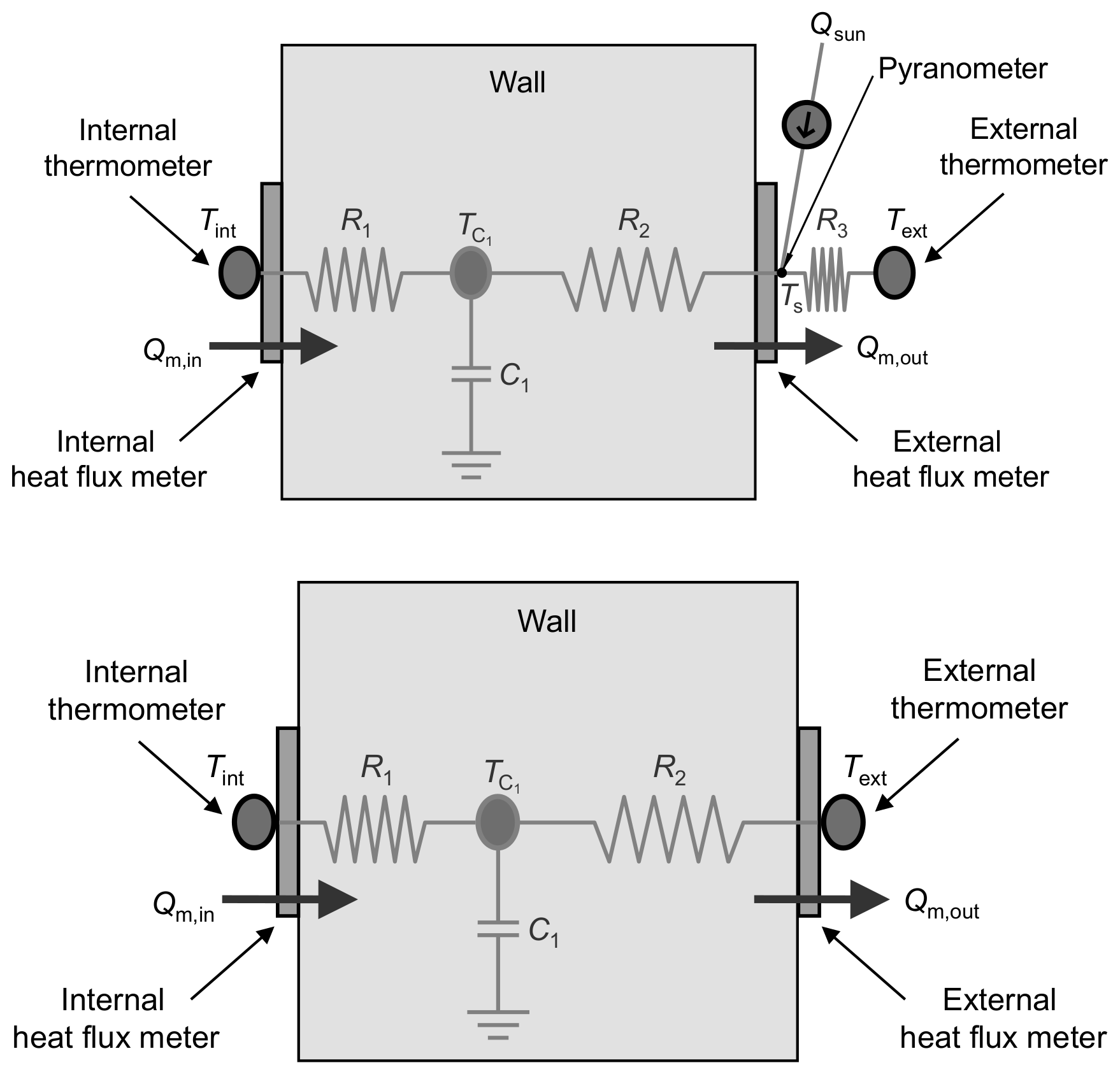
2.2. Dynamic Model: Lumped-Thermal-Mass Models

A family of lumped-thermal-mass models based on the electrical analogy to heat transfer was developed to describe the dynamic thermophysical behaviour of the building element under study (although walls were the application for this research, the approach and techniques devised can be applied to different building elements). These models were used to predict the time series of interest (i.e., either the heat flux through the structure or the temperatures on opposite sides) and evaluate the thermophysical properties of the element by means of Bayesian inference (Section 2.3) [6,29,30]. Note that in this paper, the term “predict” is used in its statistical meaning of estimating the value of a random variable rather than as a synonym of forecast, which implies making a prediction of the value of the variable at a given time in the future.

Figure 2 illustrates a one thermal mass model (1TM) explicitly incorporating solar radiation as a separate source of heat. The heat flow entering the internal $\left(Q_{\mathrm{e},\mathrm{in}}^p\right)$ and leaving the external $\left(Q_{\mathrm{e},\mathrm{out}}^p\right)$ surface at each time step can be estimated from the lumped-mass model , adopting a convention of heat flow from the internal to the external environment; although measured temperatures are used in this paper as driving forces, the method devised also allows the use of heat flux measurements for the estimation of temperature profiles. For the 1TM model including solar radiation, the model is described by Equation (2) (refer to [30] for the full derivation):

$$Q_{\mathrm{e},\mathrm{in}}^p=\frac{T_{\mathrm{int}}^p-T_{C_1}^p}{R_1},Q_{\mathrm{e},\mathrm{out}}^p=\frac{T_{C_1}^p-T_{\mathrm{ext}}^p-R_3{Q}_{\mathrm{sun}}^p}{R_2+R_3},$$

(2)

where $R_1$, $R_2$, $R_3$ are the lumped thermal resistances of the element; $T_{C_1}^p$ is the temperature of the effective thermal mass at each time step; $Q_{\mathrm{sun}}^p$ is the incoming solar radiation at each time step. The heat flow for the 1TM model without solar radiation is obtained from Equation (2) by setting $R_3$ to zero [29,30]. While either surface or air temperature can be used on the internal side for both models, surface temperature can only be used on the external side when solar radiation is not accounted for separately.

More complex models can be easily devised by expanding the 1TM models in Figure 2 using an increasing number of equivalent electrical components and extending the mathematical approach. Lumped-thermal-mass models including between zero and four effective thermal masses—both with and without the explicit incorporation of solar radiation—were developed in this research (refer to [6] for a pure resistive model, to [29] for a model including two effective thermal masses and four thermal resistances without the explicit incorporation of solar radiation (i.e., two thermal mass model, 2TM), and to [30] for all other models). These models may provide a better description of the thermal structure of the building element, such as in the case of more complex structures. The inclusion of a second thermal mass from the 1TM to the 2TM models can significantly improve the characterisation of the observed thermal performance at both the external and internal surfaces. However, in the absence of further data streams, more complex models (e.g., three and four thermal mass models) may provide more limited explanatory power. These latter models are being successfully applied in complementary research where, for example, the heat transfer through the element is used to estimate the measured temperatures. Accordingly, only the results for the 1TM and the 2TM models are presented in this paper.

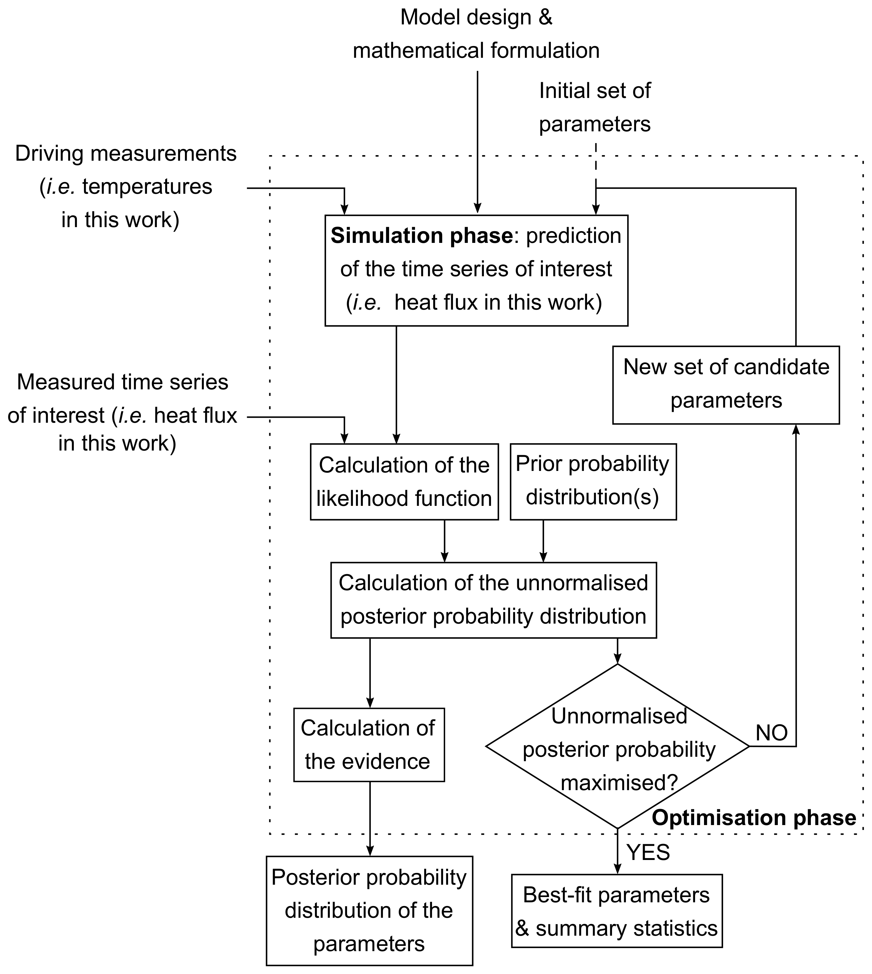
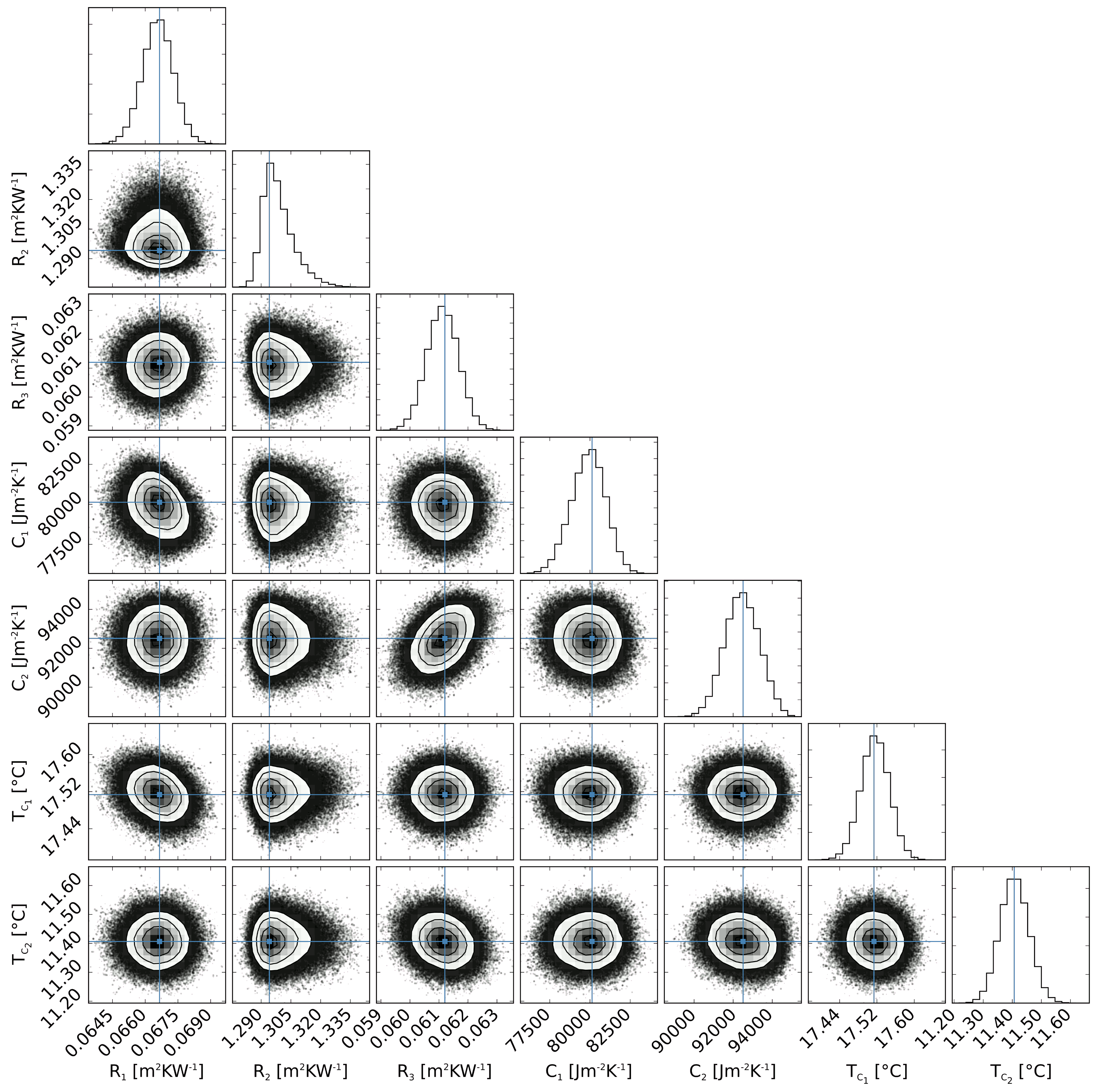
2.3. Bayesian Inference: Optimisation Phase for Thermophysical Parameter Estimation

According to Bayes theorem, the posterior probability distribution of the parameters (i.e., the probability of the parameters $\theta$ given the observations y and the model H) can be calculated as:

$$\mathbb{P}\left(\theta \mid y,H\right)=\frac{\mathbb{P}\left(y\mid \theta ,H\right)\mathbb{P}\left(\theta \mid H\right)}{\mathbb{P}\left(y\mid H\right)},$$

(3)

where $\mathbb{P}\left(y\mid \theta ,H\right)$ is the likelihood function (i.e., the probability model expected to describe the process of interest); $\mathbb{P}\left(\theta \mid H\right)$ is the prior probability distribution; and $\mathbb{P}\left(y\mid H\right)$ is the evidence (or marginal likelihood). While Bayesian approaches often consider the full posterior probability distribution, one may also be interested in knowing the best set of the parameters of interest (${\theta }_{\mathrm{opt}}$; i.e., those maximising the posterior probability distribution):

$${\theta }_{\mathrm{opt}}=\underset{\theta }{argmax}\mathbb{P}\left(\theta \mid y,H\right)=\underset{\theta }{argmax}\frac{\mathbb{P}\left(y\mid \theta ,H\right)\mathbb{P}\left(\theta \mid H\right)}{\mathbb{P}\left(y\mid H\right)}.$$

(4)

The unnormalised posterior probability distribution of different possible lumped-thermal-mass models was optimised to estimate the best-fit thermophysical parameters (as illustrated below), while the full posterior probability distribution was analysed for model comparison ([34], Chapter 28) to evaluate the relative performance of the different lumped-thermal-mass models investigated (Section 2.4.1). Maximum a posteriori (MAP) and a Markov chain Monte Carlo (MCMC) sampling were adopted as alternative options for parameter optimisation. While the former approach only estimates the best-fit value of the parameters by maximising the posterior probability distribution (i.e., identifying its mode), the latter estimates the full probability distribution of the parameters and may provide further thermophysical insights (e.g., highlighting dependencies among the parameters). The whole framework was implemented in Python 3.0 [35] using the Python SciPy “basinhopping” function [36] for MAP optimisation, and the Python library “EMCEE” [37] for MCMC sampling.

2.3.1. Likelihood Function

The likelihood function was formulated using physically informed lumped-thermal-mass models to simulate the heat transfer through the building element from in-situ measurements (according to Section 2.2), and an error model of the discrepancies between the observed and predicted time series (i.e., the residuals). Either the internal heat flux data stream, the external one, or both simultaneously (Equation (2)) can be optimised during model fitting [29].

Two different error models were implemented as alternative options. The first one adopts the common assumption of white noise residuals ([38], Chapter 5.3). Confounding physical effects such as unaccounted for environmental conditions including the impact of wind or driving rain may break the assumption of independent and identically distributed (iid) residuals and may require averaging the data over longer time steps (or other methods) to remove temporal correlation in the data. To resolve this issue and retain use of all the granularity of the dataset and minimise the loss of dynamic information, the second method uses the Bayesian framework to relax the strong assumption of iid residuals by introducing a prior distribution on them to account for potential autocorrelation.

Independent and Identically Distributed Residuals

Under the iid assumption, the residuals of each data stream contributing to the fit (i.e., the heat flux(es) in this application) can be modelled as an additive white Gaussian noise [29,38], and their probability density function is a multivariate Gaussian distribution $\left(\mathcal{N}\right)$ with zero mean and diagonal covariance matrix ${\mathrm{\Sigma }}_{\epsilon }={\sigma }_{\mathsf{\Phi },\epsilon }^2{I}_n$:

$$r_{\epsilon }\sim \mathcal{N}\left(0_n,{\sigma }_{\mathsf{\Phi },\epsilon }^2{I}_n\right),$$

(5)

where $r_{\epsilon }$ is the vector of the residuals of each data stream $\epsilon$ contributing to the fitting, with elements $r_{\epsilon }^p=\left({\mathsf{\Phi }}_{\mathrm{e},\epsilon }^p-{\mathsf{\Phi }}_{\mathrm{m},\epsilon }^p\right)$ (${\mathsf{\Phi }}_{\mathrm{e},\epsilon }^p$ and ${\mathsf{\Phi }}_{\mathrm{m},\epsilon }^p$ are respectively the estimates from the lumped-thermal-mass model and the in-situ measurement for each data stream at each time step; i.e., the estimated $\left\{Q_{\mathrm{e},\mathrm{in}}^p,Q_{\mathrm{e},\mathrm{out}}^p\right\}$ and the observed $\left\{Q_{\mathrm{m},\mathrm{in}}^p,Q_{\mathrm{m},\mathrm{out}}^p\right\}$ heat fluxes in this work); ${\sigma }_{\mathsf{\Phi },\epsilon }^2$ is the variance of an additive noise term affecting each measured data stream(s) that accounts for all sources of uncertainties affecting the observations (see Section 3.4 for the calculation of ${\sigma }_{\mathsf{\Phi },\epsilon }^2$ in the context of this work); $I_n$ is an identity matrix of dimension n (i.e., the number of observations for each data stream). Therefore, the likelihood can be expressed as:

$$\mathbb{P}\left(r\mid \theta ,H\right)=\prod _{\epsilon \in E}\frac{1}{{\left[\sqrt{2\pi {\sigma }_{\mathsf{\Phi },\epsilon }^2}\right]}^n}exp\left[-\frac{1}{2}\sum _i\frac{r_{\epsilon ,i}^2}{{\sigma }_{\mathsf{\Phi },\epsilon }^2}\right]=\prod _{\epsilon \in E}{\left(2\pi \right)}^{-\frac{n}{2}}{\left|{\mathrm{\Sigma }}_{\epsilon }\right|}^{-\frac{1}{2}}exp\left(-\frac{1}{2}{r}_{\epsilon }^{\mathrm{T}}{\mathrm{\Sigma }}_{\epsilon }^{-1}{r}_{\epsilon }\right),$$

(6)

where E is the set of data streams optimised.

Discrete Cosine Transform

Applying the Bayesian framework, the iid assumption of the residuals for each data stream can be relaxed by assuming that their probability density function is a multivariate Gaussian distribution with zero mean and unknown covariance matrix ${\mathrm{\Sigma }}_{\epsilon }$ accounting for correlation between observations. Given the temporal structure of the residuals, it is reasonable to assume that the random process generating $r_{\epsilon }$ is weakly stationary (i.e., the covariance between any two residuals only depends on the time elapsed between the two observations). Since the covariance matrix of a weakly stationary discrete-time random process is a symmetric Toeplitz matrix, this distinctive structure can be accounted for in the analysis by imposing a prior distribution on the unknown covariance matrix ${\mathrm{\Sigma }}_{\epsilon }$.

The covariance matrix of a weakly stationary discrete-time random process can be asymptotically diagonalised by the application of a discrete cosine transform (DCT) [39,40], representing a finite signal as a sum of cosine functions at different frequencies. Expressing the DCT as a matrix multiplication with the ortho-normal DCT basis matrix D, the decorrelation property of the DCT can be stated as:

$$r_{\epsilon }\sim \mathcal{N}\left(0_n,{\mathrm{\Sigma }}_{\epsilon }\right)\mathrm{with}{\mathrm{\Sigma }}_{\epsilon }=D^{\mathrm{T}}{\mathsf{\Xi }}_{\epsilon }D,$$

(7)

where ${\mathsf{\Xi }}_{\epsilon }$ is a diagonal matrix. Replacing ${\mathsf{\Xi }}_{\epsilon }$ from Equation (7) in Equation (6), the likelihood of the residuals can be rewritten in terms of the matrix ${\mathsf{\Xi }}_{\epsilon }$ and its diagonal elements. Placing a prior on ${\mathsf{\Xi }}_{\epsilon }$ indirectly places a prior on ${\mathrm{\Sigma }}_{\epsilon }$ that accounts for the desired asymptotic Toeplitz structure, which is typical of stationary signals. The likelihood function can therefore be calculated by marginalising out the unknown covariance matrix ${\mathrm{\Sigma }}_{\epsilon }$ (defined in Equation (7)). Specifically, a bounded and tapered inverse gamma distribution $\mathbb{P}\left(\xi \right)\propto {\xi }^{-\alpha -1}{e}^{-\beta /\xi }(1-\xi \delta )$ for $\xi \in (0,{\delta }^{-1})$ was placed on each diagonal element ${\xi }_{i,i}$ of ${\mathsf{\Xi }}_{\epsilon }$ [30].

2.3.2. Prior Probability Distributions on the Parameters of the Model

Prior information, introduced through the Bayesian method, may be used to reduce the number of observations needed to estimate the thermophysical properties of in-situ building elements compared to methods that do not include such information (e.g., the maximum likelihood method). This may extend the survey period to non-winter seasons, as it may reduce the required duration of monitoring campaigns, which can minimise the disruption for the occupants, meet the tight timescales of building constructions, and provide a method to investigate the time variance of estimated thermophysical properties due to environmental changes.

Both uniform and non-uniform (i.e., log-normal) priors on the parameters and the estimates (e.g., the U-value) of the model were implemented [30]; Section 3.2 discusses the definition of the priors used in this paper for the case studies analysed. To avoid imposing a correlation structure of the parameters (which may not be known a priori), the priors were assumed independent (i.e., $\mathbb{P}\left(\theta \mid H\right)={\prod }_j\mathbb{P}\left({\theta }_j\mid H\right)$). However, this choice does not prevent the model from the identification of correlations in the estimates, should the data support it.

Uniform Priors

Uniform priors were adopted when limited initial knowledge about the parameters of the model was available:

$$\mathbb{P}\left({\theta }_j\mid H\right)={\left(\Delta L_j\right)}^{-1},$$

(8)

where $\Delta L_j$ is the width of the prior on the j-th parameter. Care was taken to ensure that any reasonable value the parameters may assume was included in the uniform prior range.

Log-Normal Priors

Log-normal priors were adopted when more information on the parameters (or the estimates) of the model were available. Log-normal priors were selected in this application, as their distribution over the positive reals reflects the strictly positive property of the parameters such as the thermal resistance and the effective thermal mass of the element; this requirement is also satisfied for the initial temperature of the effective thermal mass(es) once the temperature observations are transformed from degrees Celsius to Kelvin. The log-normal scale also provides a more realistic description of the knowledge on the degree of magnitude of the random variable (i.e., the parameter) compared to a linear scale [41] as, for example, it assigns equal probability to values smaller than half the median and to those larger twice the median. Another advantage of selecting log-normal priors is represented by the distinctive property that imposing a log-normal distribution on a parameter implicitly implies a log-normal prior on its inverse (which is not necessarily true for other families of distributions). This is particularly interesting in this application given that building elements may be either modelled in terms of thermal resistance or thermal conductance.

A non-canonical parametrisation of the location parameter of the log-normal distribution ([34], Chapter 23) was adopted, where the median of the distribution of each parameter $\left(L_{{\theta }_j}\right)$ was used instead of the commonly used mean of the natural logarithm of the distribution of the parameters:

$$\mathbb{P}\left({\theta }_j\mid H\right)=\frac{1}{\sqrt{2\pi }{\theta }_j{D}_{{\theta }_j}}exp\left[-\frac{{ln}^2\left({\theta }_j/L_{{\theta }_j}\right)}{2D_{{\theta }_j}^2}\right],$$

(9)

where $L_{{\theta }_j}$ and $D_{{\theta }_j}$ are respectively a measure of location and dispersion of the log-normal distribution of the j-th parameter, based on prior knowledge. The use of the median instead of the mean is a more robust measure of location (e.g., to outliers) in case the prior distribution of the parameters is estimated from observations. Additionally, it allows the model and the corresponding location parameter to have the same units, easing the interpretation of results.

2.4. Model Selection and Validation

The six criteria for model selection and validation identified by Norlén [42] (as cited by Jiménez et al. [11]) were considered in this work. In particular, simplicity was tested using Bayesian model comparison (Section 2.4.1) to identify the simplest theory explaining the heat transfer through the building element in light of the observations; internal validity was investigated by means of cross-validation techniques (Section 2.4.2) to ensure that the performance of the best model is generalisable to new data, trustable, and replicable ([43], Chapter 7). Tests on the residuals (e.g., autocorrelation function or cumulated periodogram ([38], Chapter 6.6)) were not required after the model-fitting process, as the DCT likelihood allows the model to account for potential autocorrelation of the residuals.

2.4.1. Model Comparison

The odds ratio ([34], Chapter 28) (incorporating the Occam’s razor principle, or principle of parsimony) was used to compare the plausibility of different models fitted to their optimal parameters [6,29]:

$$\frac{\mathbb{P}\left(H_1\mid y\right)}{\mathbb{P}\left(H_2\mid y\right)}=\frac{\mathbb{P}\left(y\mid H_1\right)\mathbb{P}\left(H_1\right)}{\mathbb{P}\left(y\mid H_2\right)\mathbb{P}\left(H_2\right)},$$

(10)

where $H_1$, $H_2$ are the models to be compared; $\mathbb{P}\left(H_1\mid y\right)$, $\mathbb{P}\left(H_2\mid y\right)$ are the posterior probability distribution of each model; $\mathbb{P}\left(y\mid H_1\right)$, $\mathbb{P}\left(y\mid H_2\right)$ are the evidence of each model (whose ratio is known as “Bayes factor”); $\mathbb{P}\left(H_1\right)$, $\mathbb{P}\left(H_2\right)$ are the priors of each model (in case one of the two models is known to be more probable than the other). Depending on the optimisation framework adopted (i.e., MAP or MCMC), different methods were used to marginalise over the parameters and calculate the evidence.

For MAP estimation, the evidence of each model was calculated by marginalising over the parameters and approximating the integral by means of the Laplace method [29,34]:

$$\mathbb{P}\left(y\mid H\right)\approx \mathbb{P}\left(y\mid {\theta }_{\mathrm{MAP}}H\right)\mathbb{P}\left({\theta }_{\mathrm{MAP}}\mid H\right){\left[det\left(2\pi A\right)\right]}^{1/2},$$

(11)

where $\mathbb{P}\left(y\mid {\theta }_{\mathrm{MAP}}H\right)$ is the best-fit likelihood (i.e., the likelihood calculated for ${\theta }_{\mathrm{opt}}\equiv {\theta }_{\mathrm{MAP}}$); $\mathbb{P}\left({\theta }_{\mathrm{MAP}}\mid H\right){\left[det\left(2\pi A\right)\right]}^{1/2}$ is the Occam’s factor, where $\mathbb{P}\left({\theta }_{\mathrm{MAP}}\mid H\right)$ is the prior probability and ${\left[det\left(2\pi A\right)\right]}^{1/2}$ is a coefficient depending on the curvature of the posterior probability distribution around the global optimum.

For the MCMC approach, the evidence was calculated from the posterior density function at each step of the chain [30]. An estimator of the evidence was defined based on the reciprocal importance sampling method, which uses samples of the unnormalised posterior generated during model fitting [44]. Specifically, the estimator of the evidence was calculated as:

$$\widehat{\mathcal{Z}}={\left\{\frac{1}{m}\sum _{\theta \in B}\frac{1/v}{h\left(\theta \mid y\right)}\right\}}^{-1},$$

(12)

where m is the number of samples used to define the estimator; B is an ellipsoid centred at the MAP with shape factor according to the Hessian and radius so as to contain only the points with unnormalised posterior greater than half the value at the mode; v is the volume of the ellipsoid containing the samples from the unnormalised posterior; $h\left(\theta \mid y\right)$ is the unnormalised posterior of the parameters at each time step of the chain.

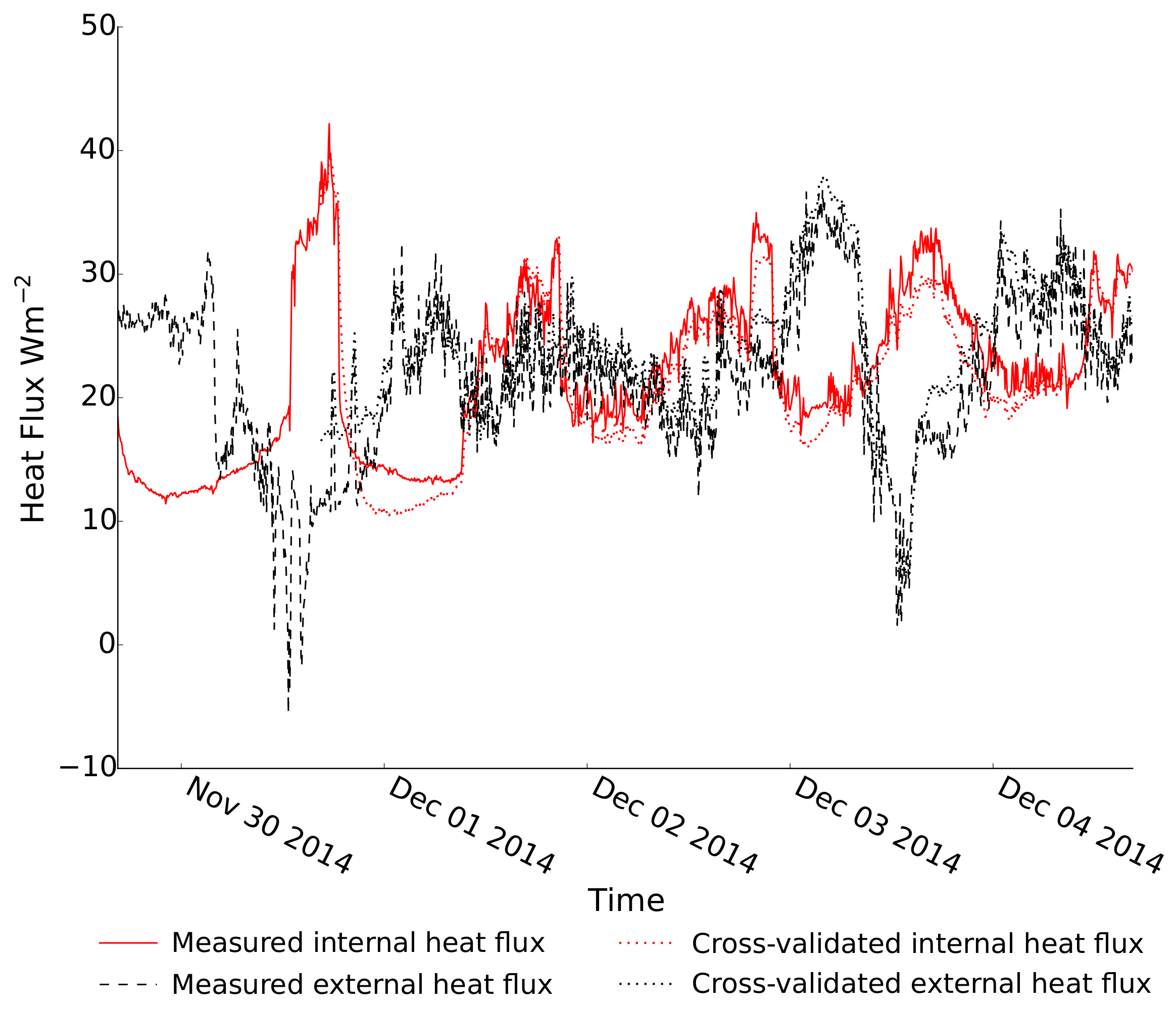
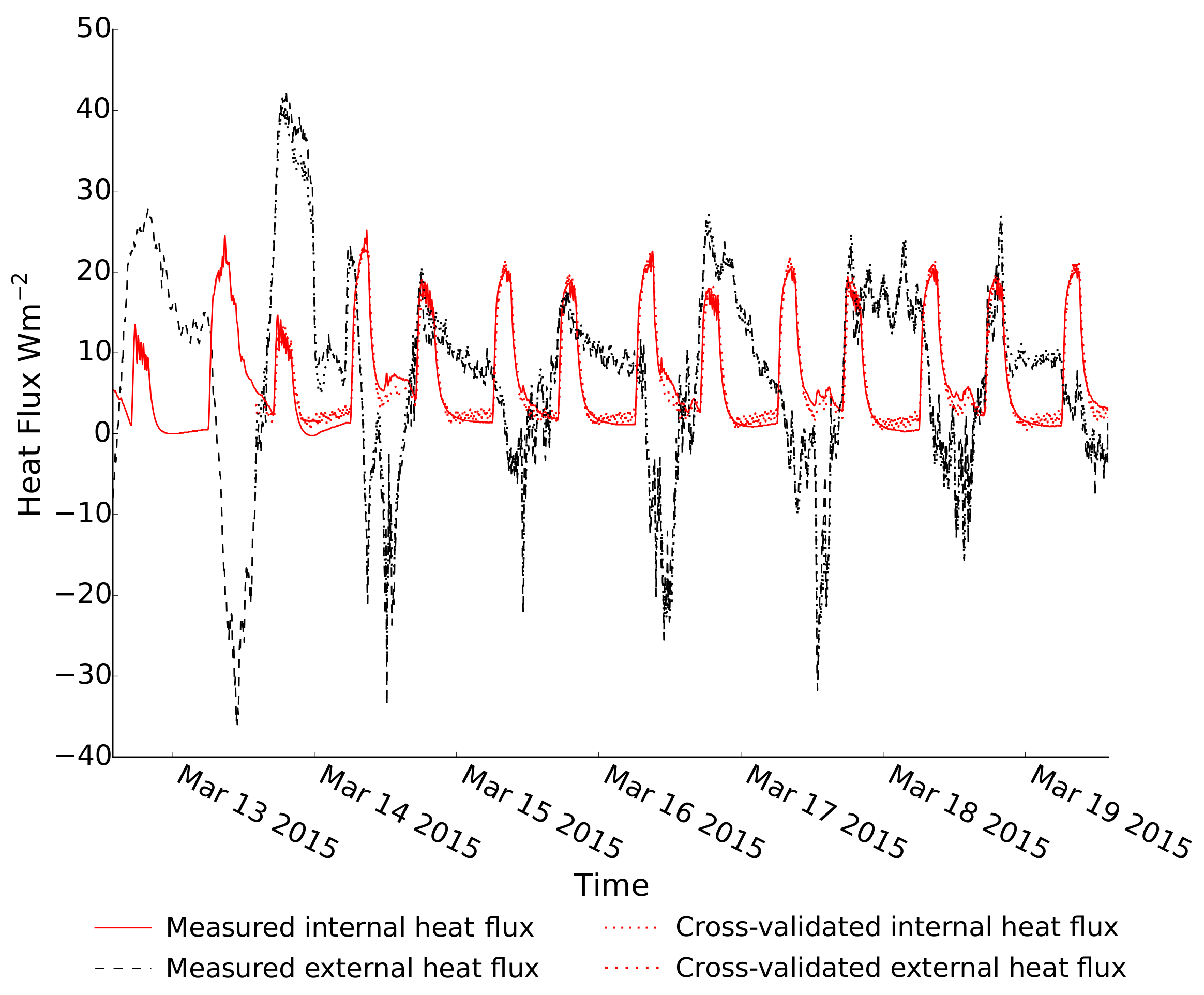
2.4.2. Cross-Validation

The best model selected was validated to test its predictive performance ([43], Chapter 7) on an independent data set to that used for model fitting. Cross-validation analysis (e.g., k-fold) is generally difficult to perform in time series analyses and intrinsically ordered data, due to the requirement of independence of the test and training sets. In the context of this research, an additional difficulty in performing cross-validation arises from the fact that the initial temperature of the thermal mass is one of the parameters of the model, and consequently the initial part of the time series cannot be used for testing purposes.

A revised k-fold cross-validation method is proposed to account for the aforementioned limitations. The requirement of independence of the training and test sets was mitigated by subdividing the time series into 24-h-long folds (under the assumption that autocorrelation is negligible after a full-day period), and leaving out the training set one fold before and one fold after the test set (as a buffer). Additionally, to obviate the issue with the estimation of the initial temperature of the thermal mass, the whole time series was used in the simulation phase but only the training set was used for optimisation purposes (i.e., parameters were estimated maximising the posterior probability on the training set only). Once the best-set parameters were identified, the cross-validation prediction error (i.e., the mean square root error of the residuals) was estimated on the test-set fold only. To enable the estimation of the initial temperature of the thermal mass, the first fold was never used as a test set.

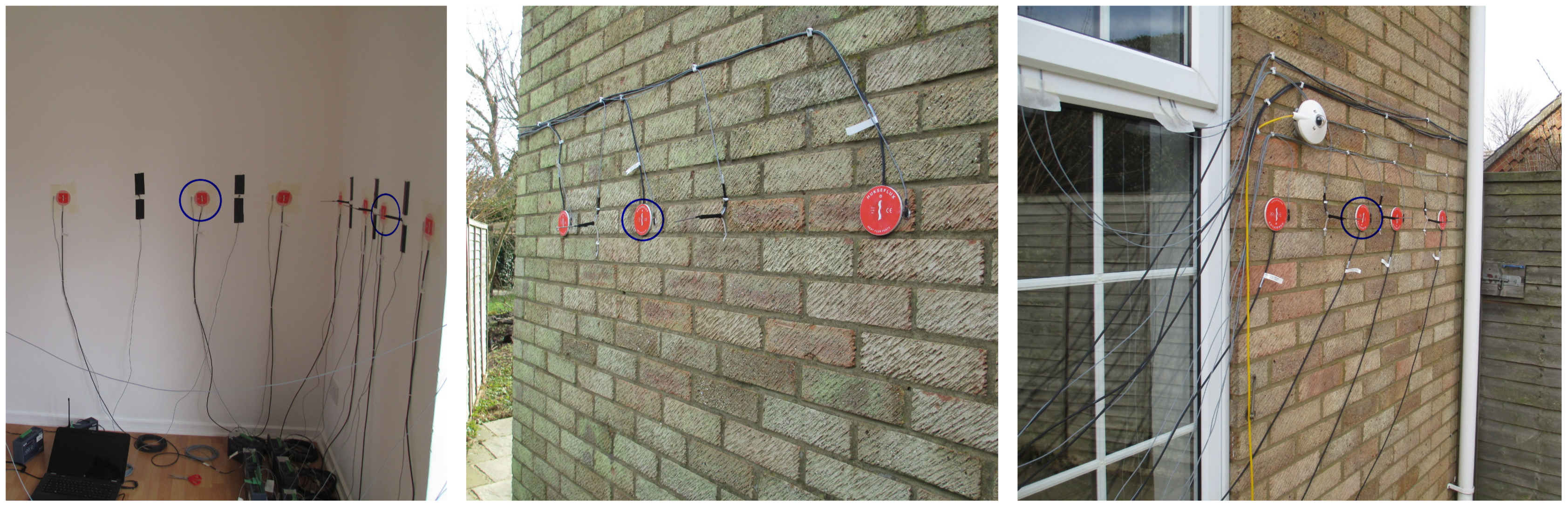
3. Experimental Data Collection and Analysis

The case studies used to test the dynamic method are presented below. This is followed by a discussion on the definition of priors, the stabilisation criteria applied, and the uncertainties and systematic errors associated with the measurement campaigns in the context of this study.

3.1. Case Studies

Two case-study buildings of solid brick and cavity wall construction were used to test the performance of the dynamic grey-box method presented. The solid brick element (SWall) constituted the external north-west-facing wall of a detached office building in central London, UK (Figure 3). The office was occupied during the data collection and no control of the heating pattern was imposed as part of the experiment, to reflect the real use of the space. The wall was $\left(370\pm 7\right)$ mm thick in total, and consisted of a $\left(20\pm 5\right)$ mm layer of plaster (expected to be lime) on the inside followed by $\left(350\pm 5\right)$ mm of exposed solid brick masonry. Pairs of heat flux plates (HFPs) [45] and type-T thermocouples were installed in-line with each other on opposite sides of the wall (refer to [29] for full details on the fixing method). The data were collected using a Campbell Scientific CR1000 [46] datalogger, averaging 5-s samples over 5-min intervals.

Two walls of nominal full-fill cavity construction (one east-facing, CWall_E, and one north-facing, CWall_N) were monitored on a 1970s detached house in Cambridgeshire, UK (Figure 4). The dwelling was unoccupied during the monitoring period and the indoor ambient was constantly heated by means of the incumbent heating system, with a set-point temperature of 20 ${}^{\circ }\mathrm{C}$. The CWall_E wall was $\left(283\pm 10\right)$ mm thick while the CWall_N was $\left(275\pm 10\right)$ mm. Detailed visual inspection showed that the walls were made of (from the inside) a layer of plaster ($\left(10\pm 5\right)$ mm), followed by a layer of aerated concrete blocks ($\left(100\pm 5\right)$ mm), a cavity originally fully filled with insulation (likely to be urea formaldehyde foam; the insulating material was assumed both from visual inspection and the year of installation (1979) reported on an original certificate of the post-built cavity-insulation intervention), and a layer of exposed brick ($\left(100\pm 5\right)$ mm). Visual inspection suggested that the insulation layer may have shrunk inside the cavity, and the thermal resistance of the walls is expected to have been decreased accordingly. Pairs of HFPs [45] and thermistors (both measuring surface and air temperature) were mounted on the two walls, and a pyranometer [47] was fixed on the CWall_E to record the incident vertical solar radiation. Data were sampled every 5 s and averaged over 5-min intervals using Eltek 451/L and 851/L dataloggers [48] for the HFPs and thermistors, while an Eltek RX250AL logger [49] sampling every 30 s and averaging over 5-min intervals was used for the pyranometer.

3.2. Definition of Priors

Log-normal priors on the parameters of the model were defined for the solid wall, while uniform priors were used for the cavity walls due to unavailability of readily available distributions in the literature for the thermophysical properties of some of the materials constituting this structure. Although it would be in principle possible to build the missing distributions by collecting a large sample of tabulated thermophysical properties for the relevant materials, this possibility was excluded due to potential theoretical issues. Since the source of tabulated values is generally omitted, the merged data may end up accounting as independent pieces of information that actually come from the same source (i.e., redundant dataset) and be affected by higher uncertainties [50]. For this reason, the thermophysical property distributions in [51] were not used in this work, as the data set in [52] used to extrapolate them did not investigate the redundancy (and consequently the reliability) of the sources [50].

Uniform Prior Distributions on the Parameters of the Model

Large uniform priors were adopted for the CWall_N and CWall_E to cover all physically plausible properties and reduce the possibility of selecting ranges that exclude rare but possible events. The thermal resistances ranged in $\left[0.01,4.00\right]$ ${\mathrm{m}}^2\mathrm{K}{\mathrm{W}}^{-1}$, the effective thermal mass(es) ranged in $\left[0.1,2.0\times {10}^6\right]$ $\mathrm{J}{\mathrm{m}}^{-2}\mathrm{K}{}^{-1}$, and their initial temperature between $\left[-5,40\right]$ ${}^{\circ }\mathrm{C}$.

Log-Normal Prior Distributions on the Parameters of the Model

Log-normal priors were defined for the SWall as follows. For the R-values and effective thermal mass(es), the location and dispersion of the log-normal prior distributions were calculated from the mean and standard deviation of the normal distributions in [50] for the thermophysical properties of the materials constituting the wall. For the initial temperatures of the thermal mass(es), the location of the log-normal priors for each month were defined from the hourly air temperature observations in the test reference year for London [53], while the dispersion was chosen to cover a range of reasonable values for this application.

Since all the thermophysical parameters involved are a function of two (or more) measured quantities (i.e., the R-value and effective thermal mass are calculated from the thermophysical properties of each layer as the SWall is a multi-layer element, while the initial temperature of the thermal mass is calculated aggregating hourly air temperature observations over one-month periods), the mean and variance of the resulting Gaussian distributions can be determined according to linear propagation of error theory [54]. Assuming that in first approximation the measurements taken to build the distribution of the thermophysical properties are independent, the mean $\left({\mu }_y\right)$ and variance $\left(v_y\right)$ of the combined function of interest can be computed as:

$${\mu }_y=\mathbb{E}\left[y\left(x_1,\dots ,x_n\right)\right]\approx y\left({\mu }_{x_1},\dots ,{\mu }_{x_n}\right),v_y=\mathbb{E}{\left(y-{\mu }_y\right)}^2\approx {\displaystyle \sum _{i=1}^n}{\left(\frac{\partial y}{\partial x_i}\right)}^2{v}_{x_i},$$

(13)

where ${\mu }_y$ is the mean of the combined distribution of the measured quantities $x_i$, and $v_y$ is its variance. The location $\left(ln{L}_Y\right)$ and dispersion $\left(D_Y\right)$ of the log-normal prior can be then obtained as:

$$D_Y=\sqrt{ln\left(1+\frac{v_y}{{\mu }_y^2}\right)},ln{L}_Y=ln{\mu }_y-\frac{1}{2}{D}_Y^2.$$

(14)

In this work, the mean and variance of the R-value (R) and effective thermal mass(es) ($\kappa$) for the multi-layer element are calculated applying Equation (13) to their definitions:

$$R={\displaystyle \sum _{i=1}^n}\frac{d_i}{{\lambda }_i},\kappa ={\displaystyle \sum _{i=1}^n}\left(d_i{\rho }_i{c}_i\right),$$

(15)

where for each layer i: $d_i$ is its thickness; ${\lambda }_i$ its thermal conductivity; ${\rho }_i$ its density; $c_i$ its specific heat capacity.

The estimators of the log-normal distribution of the lumped thermophysical parameters were identified by fixing the position of the effective thermal mass(es) first, according to the effective thickness method described in the EN ISO 13786 ([55], Appendix A) Standard. Once the thermal mass(es) were fixed, the Gaussian mean and variance of each lumped parameter (and consequently the location and dispersion of the log-normal distributions) were calculated accounting for the thermophysical properties of the material(s) contributing to it. Similarly, the location and dispersion of the air temperature for the month when the monitoring campaign started was calculated as a proxy for the log-normal prior(s) on the initial temperature of the thermal mass.

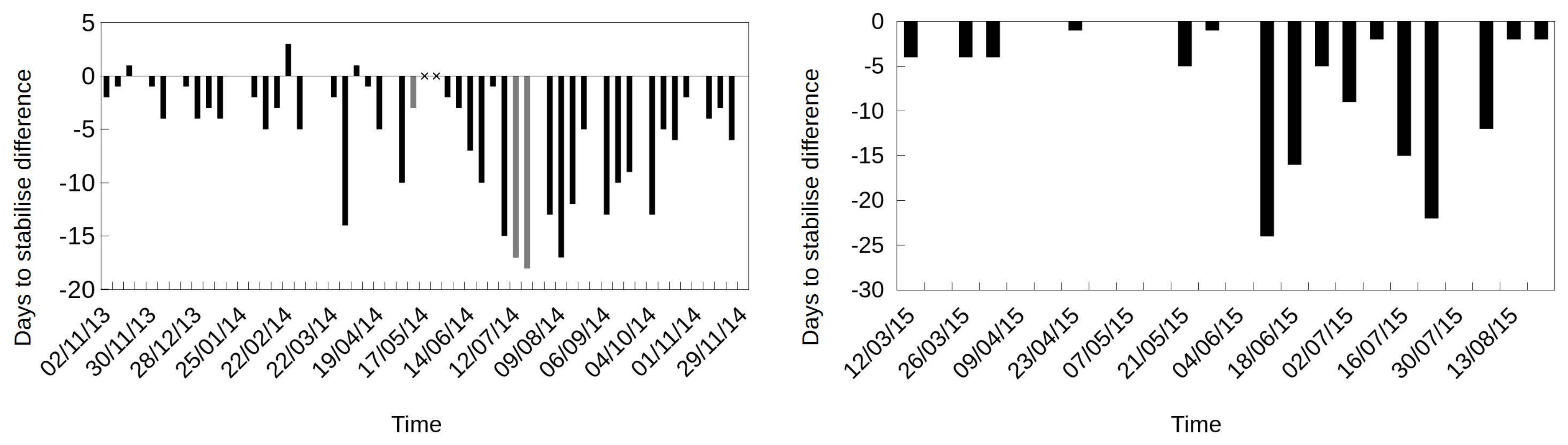
3.3. Stabilisation Criteria and Monitoring Campaign Length

The appropriate length of monitoring campaigns was determined to ensure that the parameters estimated are robust and representative of the actual thermophysical behaviour of the case study. Two contrasting requirements have to be balanced, as the time series needs to be sufficiently long to ensure that the estimates have small variability, but short enough to ensure that the assumption of a unique model to explain the data (i.e., constant parameters over the monitoring period) holds [56]. Practically, short monitoring campaigns are preferable to minimise inconvenience to the occupants, ease the integration of in-situ monitoring within building practices (e.g., for compliance and certification purposes), and constrain survey costs.

The concept of “stabilisation” is used below to refer to the identification of the minimum number of observations that must be analysed to obtain robust estimates [30,56]. The stabilisation time is the duration after which the parameter estimate is considered representative of the long-term estimate. Parameter estimates therefore avoid overfitting data to noise, while the supplement of new observations does not enhance the parameter prediction significantly; the values stabilise around a final value.

A number of stabilisation criteria are listed in the ISO 9869-1 ([18], p. 9) Standard to ensure that the assumptions underlying steady-state approaches hold for the period surveyed. Conversely, no standardised criteria are available (to the authors knowledge) for dynamic methods. Therefore, the criteria in [18] were imposed as a conservative approach to determine also the length of the time series to be analysed with the dynamic framework, although the test may be too conservative in this case [30].

To evaluate the performance of the dynamic method and test its ability to overcome the limitations of the incumbent method (discussed in Section 1), the stabilisation criteria were also applied to long-term monitoring campaigns to extract shorter time series replicating the case where surveys were performed at different times of the year (referred to as “hypothetical monitoring campaigns” [56]). Specifically, each time series started one week apart and lasted until the stabilisation criteria were met [56] according to the following scenarios. The first scenario fixed the survey length according to the minimum number of days required by the AM to stabilise, and used the time series so obtained to compare the performance of the average and dynamic method (using different lumped-thermal-mass models) in terms of parameter estimates and Bayesian model comparison. The second scenario fixed the length of each hypothetical monitoring campaign according to the number of days required by each method to stabilise. This approach investigated the ability of the dynamic method to shorten the survey period while ensuring robust estimates.

3.4. Quantification of Uncertainties on in-Situ Observations

The analysis of measured data requires the identification of all quantifiable sources of uncertainties affecting the observation to estimate how these combine and propagate to the analysis estimates. Within the dynamic method, the combination of the uncertainties affecting all data streams involved in the optimisation phase is required to define the additive noise term for the calculation of the likelihood function and consequently the evidence (Section 2.3.1 and Section 2.4.1), while the combination of all data streams involved in the analysis (i.e., both simulation and optimisation phase) is needed for the quantification of the systematic measurement error affecting the estimates of the model (Section 3.5).

Several sources of measurement error on the heat flux and temperature observations were identified [57] for the experimental analysis performed, based on the declared accuracy of monitoring equipment [45,46,48,49] and the quantification of errors listed in the incumbent Standard for in-situ measurements ([18], p. 13). Specifically, a 5% error was applied to account for the effect of random variations caused by imperfect thermal contact between the sensor and the wall, and a 3% error to account for modification of the isotherms due to the presence of the HFP. The 10% error caused by variations of the temperatures and heat flow over time was only considered for the AM analysis because the dynamic method characterises such variations through the thermal mass(es), while the 5% error accounting for temperature variations within the space and differences between radiant and air temperature ([18], p.13) was omitted owing to the use of surface temperature measurements [29].

As the measurement errors above were considered independent (in line with expectations), these were combined in quadrature sum. The additive noise term in the likelihood function and the evidence was calculated considering the errors affecting the heat flux measurement, as these were the only data streams optimised in the parameter inference phase (Section 2.3). Although in principle the errors affecting temperature observations should also be considered during optimisation, our assumption is not uncommon [11,12,22] and is supported by the BS ISO 9869-1 [18] Standard, where the errors on heat flux measurements were identified as the main source of errors on the estimates. Measurement errors on all data streams (i.e., heat flux and temperature observations) were considered for the estimation of the systematic measurement error (Section 3.5).

3.5. Quantification of Systematic Measurement Errors

A method for the quantification of the systematic measurement error affecting the estimates of the thermophysical parameters obtained with the dynamic method was developed to reflect its mathematical description of heat transfer [56]. Since the dynamic analysis calculates the interior-to-exterior temperature difference at each time step instead of averaging them over the monitoring period (like the AM), its error estimates are smaller and more robust, even in periods where the average temperature differences are close to zero or present considerable diurnal swings.

The relative systematic error on the U-value estimation for the average method can be calculated as a first-order Taylor expansion of the U-value definition:

$$\frac{{\sigma }_{\mathrm{U}}}{U}=\sqrt{\frac{{\sigma }_{{\mathrm{Q}}_{\mathrm{m}}}^2}{Q_{\mathrm{m}}^2}+\frac{{\sigma }_{\mathrm{T},\epsilon }^2}{{\left(T_{\mathrm{int}}-T_{\mathrm{ext}}\right)}^2}},$$

(16)

where ${\sigma }_{{\mathrm{Q}}_{\mathrm{m}}}$, ${\sigma }_{\mathrm{T},\epsilon }$ are the systematic measurement errors on the observed heat flux and temperature data streams, respectively (characterised according to Section 3.4). Conversely, a similar approach cannot be used for dynamic methods, where the thermophysical parameters are estimated by means of optimisation techniques minimising a given cost function (e.g., Equation (4)). In this case, the systematic measurement error on the thermophysical estimates can be quantified analysing the global optimum of the unnormalised posterior probability distribution. According to the rules for error propagation, the absolute systematic measurement error on the U-value can be formally expressed as [56]:

$${\sigma }_{\mathrm{U}}=\sqrt{{\sum }_{\epsilon }{\left(\frac{\mathrm{d}{U}_{\mathrm{opt}}}{\mathrm{d}{y}_{\epsilon }}{\sigma }_{\epsilon }\right)}^2}=\sqrt{{\sum }_{\epsilon }{\left(-\frac{1}{R_{\mathrm{tot},\mathrm{opt}}^2}{\nabla }_f^{\mathrm{T}}\frac{\mathrm{d}{\theta }_{\mathrm{opt}}}{\mathrm{d}{y}_{\epsilon }}{\sigma }_{\epsilon }\right)}^2},$$

(17)

where $R_{\mathrm{tot},\mathrm{opt}}$ is the total R-value of the element; ${\sigma }_{\epsilon }$ is the systematic measurement error on each data stream (characterised according to Section 3.4).

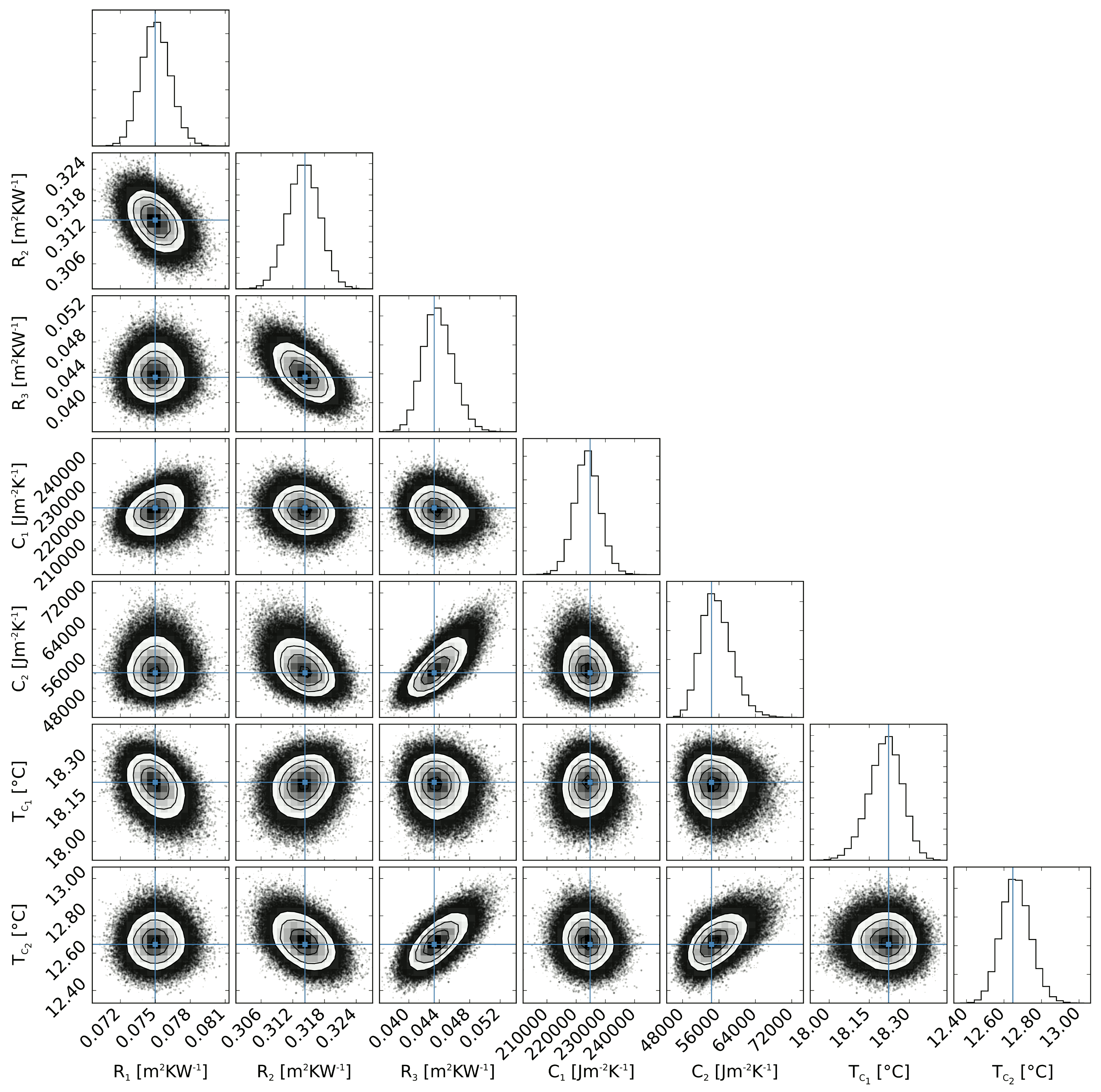
4. Results and Discussion

The three walls presented in Section 3.1 were used to investigate the performance and robustness of the dynamic models and Bayesian analysis under different conditions. Firstly (Section 4.1), it was tested according to current best practice for in-situ measurement (i.e., on north-facing elements exposed to a high temperature difference, preferably above 10 ${}^{\circ }\mathrm{C}$ [58]). The analysis was then extended to warmer seasons, initially for the two north-facing walls (Section 4.2) and subsequently for the east-facing one (Section 4.3).

4.1. Thermophysical Performance of North-Facing Walls Exposed to High Temperature Differences

The thermophysical properties of the two north-facing walls (SWall and CWall_N) were estimated according to both the average and dynamic (with the 1TM (1HF), 1TM (2HF), and 2TM models) methods using surface temperature data, and compared to the expected values from literature calculations (refer to [30] for details on the calculation of literature U-values). MCMC sampling was adopted as the optimisation framework; the mean of each parameter distribution was also calculated to ease the comparison of the results from the dynamic analysis with those from the AM and the literature. These results were cross-checked against those derived using MAP parameter estimation and were within the statistical error estimates.

4.1.1. Thermophysical Performance of the Solid Wall

Three full days of data (between 29 November and 4 December 2014, starting at 16:30 [59]) were required by the AM to meet the stabilisation criteria for the SWall. This is the shortest possible stabilisation time within the ISO 9869-1 ([18], p. 9) Standard (Section 3.3) and reflects the good conditions for such monitoring, with stable weather conditions and an average temperature difference between the two sides of the wall of $9.6$ ${}^{\circ }\mathrm{C}$ (the “average temperature difference between the two sides of the element” will be referred to as “average temperature difference” in the following for conciseness). The U-values obtained from in-situ measurements were $1.69\pm 0.25$ $\mathrm{W}{\mathrm{m}}^{-2}\mathrm{K}{}^{-1}$ with the AM, $1.75\pm 0.18$ $\mathrm{W}{\mathrm{m}}^{-2}\mathrm{K}{}^{-1}$ for the 1TM (1HF) model, $1.72\pm 0.16$ $\mathrm{W}{\mathrm{m}}^{-2}\mathrm{K}{}^{-1}$ for the 1TM (2 HF) model, and $1.69\pm 0.16$ $\mathrm{W}{\mathrm{m}}^{-2}\mathrm{K}{}^{-1}$ for the 2TM model. All values were within the margin of systematic measurement error (statistical error is significantly lower and not quoted here for clarity; see

Table 1. Thermophysical properties for the SWall for the average (AM) and dynamic (using the 1TM (1HF), 1TM (2HF), and the 2TM models) method. Only the statistical error is shown, and the number of significant figures was chosen to illustrate the level of the error.

Parameters	Literature	AM	1TM (1 HF)	1TM (2 HF)	2TM	Units
$R_1$			$0.071\pm 0.001$	$0.075\pm 0.001$	$0.075\pm 0.001$	$\mathrm{m}{}^2\mathrm{K}{\mathrm{W}}^{-1}$
$R_2$			$0.344\pm 0.002$	$0.350\pm 0.003$	$0.314\pm 0.003$	$\mathrm{m}{}^2\mathrm{K}{\mathrm{W}}^{-1}$
$R_3$					$0.044\pm 0.002$	$\mathrm{m}{}^2\mathrm{K}{\mathrm{W}}^{-1}$
$C_1$	$\left[1.08,1.80\right]\times {10}^5$		$2.25\pm 0.05\times {10}^5$	$2.28\pm 0.06\times {10}^5$	$2.24\pm 0.04\times {10}^5$	$\mathrm{J}\mathrm{m}{}^{-2}\mathrm{K}{}^{-1}$
$C_2$	$\left[1.01,1.92\right]\times {10}^5$				$0.56\pm 0.03\times {10}^5$	$\mathrm{J}\mathrm{m}{}^{-2}\mathrm{K}{}^{-1}$
$T_{{\mathrm{C}}_1}^0$			$18.24\pm 0.05$	$18.27\pm 0.06$	$18.21\pm 0.06$	${}^{\circ }\mathrm{C}$
$T_{{\mathrm{C}}_2}^0$					$12.66\pm 0.08$	${}^{\circ }\mathrm{C}$
R-value	$\left[0.29,0.73\right]$	$0.42$	$0.415\pm 0.001$	$0.425\pm 0.002$	$0.433\pm 0.002$	$\mathrm{m}{}^2\mathrm{K}{\mathrm{W}}^{-1}$
U-value	$\left[1.11,2.16\right]$	$1.69$	$1.747\pm 0.007$	$1.717\pm 0.012$	$1.694\pm 0.011$	$\mathrm{W}\mathrm{m}{}^{-2}\mathrm{K}{}^{-1}$

). A summary of the thermophysical parameter estimates and the expected values from literature calculation is reported in Table 1. The R-values and U-value estimates for the average and dynamic methods fell within the ranges calculated from the literature, while the internal and external effective thermal mass estimates obtained from the 2TM model were comparable with the calculation using tabulated values.

The full distribution of the thermophysical parameters of the 2TM model is shown in Figure 5. The corner plot shows a negative relationship among the thermal resistance estimates, as the principal axis of the contours representing the posterior probability distribution are rotated with respect to the Cartesian axes [60]. This suggests that the model derived a constant total R-value (and consequently U-value) of the wall, while the relative magnitude of each lumped thermal resistance could vary (e.g., a decrease in $R_1$ tended to be compensated for by an increase in $R_2$). Such relationships may be used to provide valuable insight into the thermal structure of the element; here the solid wall construction strongly constrains the total thermal mass and resistance, whilst the comparable thermophysical properties of the materials in the wall only weakly constrain the position of two effective thermal masses in thermal resistance space [60].

Model selection was performed to investigate the relative plausibility of the 1TM (2HF) and 2TM models fitted to their most probable parameters. The 2TM model was identified as that more likely to describe the underlying physical process (the natural logarithm of the odds ratio was −7633 in favour of the 2TM model). Cross-validation was performed on the best model to ensure that it was also robust, generalisable, and replicable [43]. Figure 6 shows the measured and cross-validated time series, with an initial one day of training data (Section 2.4.2). The modelled and observed data match well, although the survey only lasted for three days. This result shows that the model was able to estimate the heat flux accurately on out-of-sample data using only one full day of training data.

4.1.2. Thermophysical Performance of the Cavity Wall

Seven full days of data (between 12 and 19 March 2015, starting at 14:00 [61]) were required by the AM to meet the stabilisation criteria for the cavity wall (CWall_N), and the average temperature difference was $10.0$ ${}^{\circ }\mathrm{C}$. A summary of the thermophysical parameter estimates and the expected values from literature calculation is reported in

Table 2. Thermophysical properties for the CWall_N for the average (AM) and dynamic (using the 1TM (1HF), 1TM (2HF), and the 2TM models) method. Only the statistical error is shown, and the number of significant figures was chosen to illustrate the level of the error.

Parameters	Literature	AM	1TM (1 HF)	1TM (2 HF)	2TM	Units
$R_1$			$0.066\pm 0.001$	$1.411\pm 0.004$	$0.067\pm 0.001$	$\mathrm{m}{}^2\mathrm{K}{\mathrm{W}}^{-1}$
$R_2$			$1.361\pm 0.007$	$0.062\pm 0.001$	$1.299\pm 0.008$	$\mathrm{m}{}^2\mathrm{K}{\mathrm{W}}^{-1}$
$R_3$					$0.061\pm 0.001$	$\mathrm{m}{}^2\mathrm{K}{\mathrm{W}}^{-1}$
$C_1$	$\left[0.51,0.90\right]\times {10}^5$		$0.82\pm 0.01\times {10}^5$	$0.94\pm 0.01\times {10}^5$	$0.80\pm 0.01\times {10}^5$	$\mathrm{J}\mathrm{m}{}^{-2}\mathrm{K}{}^{-1}$
$C_2$	$\left[0.96,2.08\right]\times {10}^5$				$0.92\pm 0.01$	$\mathrm{J}\mathrm{m}{}^{-2}\mathrm{K}{}^{-1}$
$T_{{\mathrm{C}}_1}^0$			$17.56\pm 0.03$	$11.39\pm 0.05$	$17.52\pm 0.03$	${}^{\circ }\mathrm{C}$
$T_{{\mathrm{C}}_2}^0$					$11.41\pm 0.05$	${}^{\circ }\mathrm{C}$
R-value	$\left[2.36,3.01\right]$	$1.47$	$1.427\pm 0.007$	$1.473\pm 0.004$	$1.427\pm 0.008$	$\mathrm{m}{}^2\mathrm{K}{\mathrm{W}}^{-1}$
U-value	$\left[0.32,0.40\right]$	$0.61$	$0.631\pm 0.003$	$0.613\pm 0.002$	$0.631\pm 0.004$	$\mathrm{W}\mathrm{m}{}^{-2}\mathrm{K}{}^{-1}$

. The U-value estimates from in-situ measurements ($0.61\pm 0.08$ $\mathrm{W}{\mathrm{m}}^{-2}\mathrm{K}{}^{-1}$ for the AM, $0.63\pm 0.06$ $\mathrm{W}{\mathrm{m}}^{-2}\mathrm{K}{}^{-1}$ for the 1TM (1HF), $0.61\pm 0.04$ $\mathrm{W}{\mathrm{m}}^{-2}\mathrm{K}{}^{-1}$ for the 1TM (2HF), and $0.63\pm 0.05$ $\mathrm{W}{\mathrm{m}}^{-2}\mathrm{K}{}^{-1}$ for the 2TM model) were all comparable but higher than the range of calculated values from literature. This is expected following visual inspection of an adjacent cross-section of the wall that indicated significant shrinkage of the insulation (Section 3.1). The internal and external effective thermal masses estimated with the 2TM model were in good agreement with the literature values. Specifically, the internal effective thermal mass was within the literature range, while the external one was slightly lower.

The full distribution of the thermophysical parameters of the 2TM model is shown in Figure 7. Unlike the SWall case study, no correlation is apparent between the lumped thermal resistances, as the principal axes of the contours representing the posterior probability distribution are not rotated with respect to the Cartesian axes [60]. Specifically, the model found the thermal resistances to be independent of each other, and consequently their position in thermal resistance space is not correlated. This can be interpreted in light of the known physical structure of the wall: the distinct thermophysical properties of the constituent materials (i.e., a layer of aerated solid brick and a layer of aerated blocks separated by a layer of insulation) is reflected in the model solution, which identified two thermal masses that are constrained in thermal resistance space, and not correlated to each other.

Similarly to the SWall, model comparison favoured the 2TM as the most representative of the heat transfer observed in-situ; the natural logarithm of the odds ratio was −7694. Cross-validation for the best model showed a good match between the measured and estimated time series (Figure 8), suggesting that the 2TM model is appropriate in this case and able to provide robust, generalisable, and replicable estimates.

4.2. Reducing the Required Monitoring Length and Temperature Difference

Two key limitations of the incumbent method for estimating the in-situ thermal performance of building elements were discussed in Section 1: the length of monitoring campaign, and the requirement for a high average internal-to-external temperature difference during the surveyed period. The ability of the dynamic grey-box method presented here to overcome these limitations is explored in this section using long-term time series collected over different seasons and a hypothetical monitoring campaign approach (described in Section 3.3).

In-situ measurements starting on 2 November 2013 and ending on 29 November 2014 were used for the SWall [59]; two weeks of data (between 16 and 30 May 2014) were excluded due to repeated missing data for the internal thermocouple. The monitoring period spanned between 12 March 2015 and 30 August 2015 for the CWall_N [61]. Initially, hypothetical monitoring campaigns whose length were determined according to the minimum number of days required by the AM to stabilise were extracted from the long-term time series. This allowed both model comparison of the different thermal mass models at different times of the year, and the estimation of the thermophysical properties of the two walls according to the AM (Section 3.3). Then, the hypothetical monitoring campaign approach was applied to extract the data according to the minimum number of days required by the best model to stabilise. This allowed the investigation of the potential of the dynamic method to shorten the monitoring period while ensuring reliable and robust estimates.

For the hypothetical monitoring campaigns determined according to the AM, 52 out of the 55 possible for the SWall met the stabilisation criteria in ([18], p. 9), while all 24 did so for the CWall_N. Model comparison selected the 2TM model as the best one at all times of the year for both walls, and all possible hypothetical monitoring campaigns stabilised for this model (for conciseness, in the following the estimates obtained from the hypothetical monitoring campaigns determined according to the minimum number of days required by the AM to stabilise will be referred to as AM estimates; similarly, for the dynamic method using the 2TM model). Figure 9 shows that for both walls the dynamic method generally considerably reduced the length of the monitoring period compared to the AM, especially during the warmer months. The number of days required by the 2TM model to stabilise spanned between 3 and 20 days for the SWall, and in the range of 3 to 30 days for the AM. For the three hypothetical monitoring campaigns where the AM did not meet the ISO 9869-1 Standard criteria (in grey in Figure 9), the minimum duration of either the number of days before missing data or a 30-day limit were considered. For the CWall_N, the 2TM model required between 3 and 8 days to stabilise, while 3 to 28 days of observations were needed for the AM. Note that a minimum of three full days is required by the ISO 9869-1 ([18], p. 9) Standard, although this may potentially overestimate the minimum number of observations needed for the dynamic method to stabilise (Section 3.3) [30].

Table 3. Minimum, maximum, mean, and standard deviation of U-value and relative systematic measurement error estimates for the SWall and the CWall_N, using the average and dynamic (2TM model) method and hypothetical monitoring campaigns of different length.

	Method	Min	Max	Mean	St Dev	Units
SWall	AM	1.28	1.92	1.71	0.14	$\mathrm{W}\mathrm{m}{}^{-2}\mathrm{K}$
	AM error	14	50	22	8	%
	2TM	1.43	1.87	1.72	0.08	$\mathrm{W}\mathrm{m}{}^{-2}\mathrm{K}$
	2TM error	8	32	15	6	%
CWall_N	AM	0.59	1.00	0.71	0.08	$\mathrm{W}\mathrm{m}{}^{-2}\mathrm{K}$
	AM error	13	21	16	3	%
	2TM	0.64	0.82	0.70	0.05	$\mathrm{W}\mathrm{m}{}^{-2}\mathrm{K}$
	2TM error	7	14	10	2	%

shows a summary of the U-value estimates and the associated relative systematic measurement errors obtained from the 2TM model and the AM across the hypothetical monitoring campaigns. For both case studies, the mean U-value obtained using the dynamic method and shorter time series was comparable to the AM estimates and within the margin of the systematic measurement error, although the variability of the dynamic U-value estimates was considerably reduced. The 2TM model also decreased both the mean (by 25% for the SWall and by 33% for the CWall_N) and the standard deviation of the relative systematic error estimates compared to the AM (Table 3). Besides summary statistics, it is interesting to investigate whether for each pair of hypothetical monitoring campaigns (i.e., surveys starting on the same day and lasting until both the 2TM model and the AM stabilised) the use of a different amount of observations affects the final U-value estimates. Figure 10 illustrates that the probability density of the relative discrepancy between U-values estimated with the two methods was generally smaller than $\pm 5\%$ in both case studies.

To investigate the robustness of the two methods to changes of the boundary conditions to which the elements are exposed, the U-value estimates from the average and dynamic methods were compared as a function of the coefficient of variation of the temperature differences observed during each hypothetical monitoring campaign (Figure 11); differences in campaign length correspond to differences in the stabilisation time. The coefficient of variation enumerates the variability of the temperature differences observed in relation to their mean, providing insight into the impact of the changeability of the conditions upon U-value estimation and error (the “coefficient of variation of the temperature differences” will be referred to as “coefficient of variation” in the following for conciseness). Figure 11 shows that U-value estimates generally presented a higher dispersion around their mean as the coefficient of variation increased, in line with increases in the estimated relative systematic error. The dynamic method provides more robust estimates both in terms of U-value and associated relative systematic measurement error, even for periods where large daily swings or small average temperatures may have occurred (i.e., high coefficient of variation values). Similarly, the modelled thermal mass distribution within the walls did not generally vary considerably throughout the measurement campaigns.

4.3. Thermophysical Performance of an East-Facing Wall

An additional limitation of the incumbent monitoring method is the requirement to undertake in-situ measurements on north-facing elements in order to avoid the dynamic effects of direct solar radiation. Given the ability of the dynamic method to deal with periods of low average temperature difference and high variability of the conditions (shown in the previous section), the analysis was extended to an east-facing element (CWall_E).

As the 2TM model was found to perform well in conditions with high coefficients of variation and low indoor-to-outdoor temperature differences (Section 4.2), it was also adopted for this analysis. The relative performance of a model explicitly including solar radiation as an additional source of heat (2TM_sun) was compared to that without (2TM) (Section 2.2, Figure 2), given the expected higher solar radiation on an east-facing wall than on a north-facing one. Similarly to the case above for north-facing walls, hypothetical monitoring campaigns of equal length and determined according to the minimum number of days required by the AM to stabilise using surface temperature measurements were adopted for this purpose.

In-situ measurements starting on 16 April 2015 and lasting until 30 August 2015 were analysed [62]; about two weeks of air temperature data (between 30 April and 15 May 2015) were excluded due to repeated missing data. Of the 19 possible hypothetical monitoring campaigns, only 13 met the stabilisation criteria according to the AM. Model comparison selected the one using surface temperatures as the best in all cases compared to the one using air temperatures and incident solar radiation as an additional heat source in the system. The result suggests that surface temperature measurements were already able to account for solar radiation, and that the additional parameter of the 2TM_sun model did not improve the fit enough to justify the extra complexity.

The hypothetical monitoring campaign approach was subsequently adopted to investigate the minimum number of days required by the best 2TM model to stabilise at different times of the year, and the robustness of the parameter estimates. Of all possible hypothetical monitoring campaigns, only two did not stabilise according to the ISO 9869-1 ([18], p. 9) Standard criteria. The monitoring length was comparable to the commonly accepted duration of winter-time monitoring campaigns using steady-state approaches on north-facing walls, spanning between 3 and 22 days. A larger number of days was required in June and July.

A summary of the U-value and relative systematic error estimates obtained across hypothetical monitoring campaigns is shown in

Table 4. Minimum, maximum, mean, and standard deviation of U-value and relative systematic measurement error estimates for the CWall_E, using the 2TM model and hypothetical monitoring campaigns of different length.

Model	Min	Max	Mean	St Dev	Units
2TM	0.68	0.92	0.77	0.05	$\mathrm{W}\mathrm{m}{}^{-2}\mathrm{K}{}^{-1}$
2TM error	5	37	16	9	%

. The estimates are within the margin of error of those obtained for the CWall_N (U-value: $\left(0.70\pm 0.05\right)$ $\mathrm{W}{\mathrm{m}}^{-2}\mathrm{K}$; relative systematic measurement error: $\left(10\pm 2\right)$%, Table 3) for hypothetical monitoring campaigns performed during the same period the CWall_E was surveyed (i.e., hypothetical monitoring campaigns starting on the same day and running until each had stabilised using the 2TM model). Although the values are not directly comparable (e.g., due to the slightly different thickness of the walls, and potential differences in boundary conditions and moisture content), the result suggests that the 2TM model may be able to extend the analysis to characterise the performance of building elements subject to direct solar radiation, even in the summer, while providing robust thermophysical estimates.

To investigate the robustness of the estimates to highly variable boundary conditions, the U-value and the relative systematic measurement error estimates were analysed as a function of the coefficient of variation of both the temperature differences and the average diurnal solar radiation (Figure 12). The “average diurnal solar radiation” (referred to as “incident solar radiation” in the following for conciseness) was calculated using a 5 $\mathrm{W}{\mathrm{m}}^{-2}$ threshold, corresponding to the pyranometer’s zero offset [47]—i.e., the amplitude of spurious readings observable even in the absence of solar radiation caused by temperature changes. Neither the coefficient of variation of the temperature differences nor the incident solar radiation exhibit a clear correlation with the U-value estimates, whilst the systematic error exhibits no clear relationship with the coefficient of variation of the incident solar radiation, but as expected becomes more variable and larger as the coefficient of variation of the temperature differences decreases.

5. Conclusions

A Bayesian grey-box dynamic method for the estimation of the thermophysical properties of building elements from in-situ-measurements was presented, and its performance was tested on walls of different construction and orientation monitored long-term. The Bayesian framework facilitated the inclusion of several features in the analysis that can improve both the robustness of estimates and the potential physical insights from interpreting the results. Firstly, the dynamic heat transfer through the structure was characterised by combining in-situ measured data and prior knowledge of the thermophysical properties of the elements surveyed by means of uniform and log-normal priors. Secondly, the probability distribution of the parameter estimates obtained from Markov chain Monte Carlo sampling provided useful insights into the thermal structure of the element in light of its actual stratigraphy. Thirdly, a discrete-cosine-transform-based prior on the residuals of the model was included in the likelihood function to account for their potential autocorrelation, obviating the common strong assumption of independent and identically distributed residuals. Finally, model comparison and cross-validation techniques allowed the identification of the best model of heat transfer among several, and tested its ability to generalise to out-of-sample data sets.

The robustness and performance of the Bayesian grey-box dynamic method was initially tested according to best practice. Two north-facing walls exposed to a high average temperature difference were analysed with the commonly used quasi-static average method (AM) [18] and the dynamic method using lumped-thermal-mass models of different complexity. The estimates obtained from the two methods were comparable, and in line with those expected from the literature and visual inspection of the case studies. Model comparison selected a model with two lumped effective thermal masses and three lumped thermal resistances (2TM model) as the most representative of the measurements.

The proposed dynamic method was tested to investigate its ability to overcome key limitations of the steady-state methods generally adopted for the analysis of in-situ measurements. Specifically, the dynamic method’s performance was tested for reducing the length of the monitoring period compared to the steady-state approach and extending the external conditions from which data may be successfully analysed. The number of days required by the 2TM model to produce a stable U-value estimate (according to the criteria in [18]) was generally lower than the AM. The 2TM model was also able to meet the stabilisation criteria in cases where the AM did not do so within a thirty day period. The dynamic method performed well in periods with low internal-to-external temperature gradients and when large daily swings in external temperature were apparent, with little variation in U-values and considerably lower systematic error than the average method. This performance extended to periods with significant direct solar radiation. Bayesian model comparison selected the 2TM model using surface temperatures above that with solar radiation explicitly included as an additional heat source, suggesting that surface temperature measurements were already accounting for solar radiation.

The 2TM model of the dynamic method, with MCMC sampling, provided useful insights into the thermophysical structure of the elements surveyed by interpretation of the probability distributions of the parameters. Specifically, covariance was observed between the three thermal resistances estimated for the 2TM model of a solid wall (with constant total resistance), while no covariance was observed for a cavity wall, highlighting the different thermal characteristics of a wall with relatively continuous properties (loose internal constraints) to one comprising layers of distinct properties (strong internal constraints). This feature of the method may be useful for the characterisation of thermal elements of unknown structure (such as some historic walls), and could be developed with additional thermal models for specific applications in the future.

The Bayesian grey-box dynamic method presented and the analysis undertaken show its potential to shorten the length of the required monitoring period compared to the incumbent steady-state method, while also decreasing the systematic error on U-value estimates. The dynamic method performed well at all times of the year, including times when the element was exposed to high incident solar radiation. A rapid and robust method to characterise the thermophysical structure of buildings may have a wide range of applications as a tool for diagnosis and performance evaluation (e.g., tailored retrofitting interventions, quality assurance, energy performance guarantee) and open new regulatory and business opportunities towards closing the performance gap.

References

1. Zero Carbon Hub. Closing the Gap between Design & As-Built Performance. End of Term Report; Technical Report; Zero Carbon Hub: London, UK, 2014. [Google Scholar]
2. IEA EBC Annex 58—Reliable Building Energy Performance Characterisation Based on Full Scale Dynamic Measurements. Available online: http://www.iea-ebc.org/projects/project?AnnexID=58 (accessed on 31 January 2018).
3. IEA EBC Annex 70—Building Energy Epidemiology: Analysis of Real Building Energy Use at Scale. Available online: http://www.iea-ebc.org/projects/project?AnnexID=70 (accessed on 31 January 2018).
4. IEA EBC Annex 71—Energy Performance Assessment Based on in-situ Measurements. Available online: http://www.iea-ebc.org/projects/project?AnnexID=71 (accessed on 31 January 2018).
5. Cesaratto, P.G.; De Carli, M. A measuring campaign of thermal conductance in situ and possible impacts on net energy demand in buildings. Energy Build. 2013, 59, 29–36. [Google Scholar] [CrossRef]
6. Biddulph, P.; Gori, V.; Elwell, C.A.; Scott, C.; Rye, C.; Lowe, R.; Oreszczyn, T. Inferring the thermal resistance and effective thermal mass of a wall using frequent temperature and heat flux measurements. Energy Build. 2014, 78, 10–16. [Google Scholar] [CrossRef]
7. Desogus, G.; Mura, S.; Ricciu, R. Comparing different approaches to in situ measurement of building components thermal resistance. Energy Build. 2011, 43, 2613–2620. [Google Scholar] [CrossRef]
8. Ficco, G.; Iannetta, F.; Ianniello, E.; d’Ambrosio Alfano, F.R.; Dell’Isola, M. U-value in situ measurement for energy diagnosis of existing buildings. Energy Build. 2015, 104, 108–121. [Google Scholar] [CrossRef]
9. McIntyre, D.A. In situ measurement of U-values. Build. Serv. Eng. Res. Technol. 1985, 6, 1–6. [Google Scholar] [CrossRef]
10. Siviour, J. Experimental U-values of some house walls. Build. Serv. Eng. Res. Technol. 1994, 15, 35–36. [Google Scholar] [CrossRef]
11. Jiménez, M.J.; Porcar, B.; Heras, M.R. Application of different dynamic analysis approaches to the estimation of the building component U value. Build. Environ. 2009, 44, 361–367. [Google Scholar] [CrossRef]
12. Naveros, I.; Bacher, P.; Ruiz, D.P.; Jiménez, M.J.; Madsen, H. Setting up and validating a complex model for a simple homogeneous wall. Energy Build. 2014, 70, 303–317. [Google Scholar] [CrossRef]
13. Deconinck, A.H.; Roels, S. A maximum likelihood estimation of the thermal resistance of a cavity wall from on-site measurements. Energy Procedia 2015, 78, 3276–3281. [Google Scholar] [CrossRef]
14. Albatici, R.; Tonelli, A.M. Infrared thermovision technique for the assessment of thermal transmittance value of opaque building elements on site. Energy Build. 2010, 42, 2177–2183. [Google Scholar] [CrossRef]
15. Nardi, I.; Paoletti, D.; Ambrosini, D.; de Rubeis, T.; Sfarra, S. U-value assessment by infrared thermography: A comparison of different calculation methods in a Guarded Hot Box. Energy Build. 2016, 122, 211–221. [Google Scholar] [CrossRef]
16. O’Grady, M.; Lechowska, A.A.; Harte, A.M. Infrared thermography technique as an in-situ method of assessing heat loss through thermal bridging. Energy Build. 2017, 135, 20–32. [Google Scholar] [CrossRef]
17. Lehmann, B.; Ghazi Wakili, K.; Frank, T.; Vera Collado, B.; Tanner, C. Effects of individual climatic parameters on the infrared thermography of buildings. Appl. Energy 2013, 110, 29–43. [Google Scholar] [CrossRef]
18. International Organization for Standardization. Thermal Insulation—Building Elements—In-Situ Measurement of Thermal Resistance and Thermal Transmittance; Part 1: Heat Flow Meter Method; BS ISO 9869-1; ISO: Geneva, Switzerland, 2014. [Google Scholar]
19. Jiménez, M.J.; Madsen, H. Models for describing the thermal characteristics of building components. Build. Environ. 2008, 43, 152–162. [Google Scholar] [CrossRef]
20. Deconinck, A.H.; Roels, S. Comparison of characterisation methods determining the thermal resistance of building components from onsite measurements. Energy Build. 2016, 130, 309–320. [Google Scholar] [CrossRef]
21. Hens, H. Building Physics—Heat, Air and Moisture: Fundamentals and Engineering Methods with Examples and Exercises; Ernst & Sohn Verlag für Architektur und technische Wissenschaften GmbH & Co. KG: Berlin, Germany, 2012. [Google Scholar]
22. Roulet, C.; Gass, J.; Marcus, I. In-Situ U-Value Measurement: Reliable Results in Shorter Time by Dynamic Interpretation of Measured Data. In Thermal Performance of the Exterior Envelopes of Buildings III; ASHRAE Transactions: Atlanta, GA, USA, 1987; pp. 777–784. [Google Scholar]
23. Kristensen, N.R.; Madsen, H.; Jørgensen, S.B. Parameter estimation in stochastic grey-box models. Automatica 2004, 40, 225–237. [Google Scholar] [CrossRef]
24. Baker, P.H.; van Dijk, H.A.L. PASLINK and dynamic outdoor testing of building components. Build. Environ. 2008, 43, 143–151. [Google Scholar] [CrossRef]
25. Kramer, R.; van Schijndel, J.; Schellen, H. Simplified Thermal and Hygric Building Models: A Literature Review. Front. Archit. Res. 2012, 1, 318–325. [Google Scholar] [CrossRef]
26. Dubois, S.; McGregor, F.; Evrard, A.; Heath, A.; Lebeau, F. An inverse modelling approach to estimate the hygric parameters of clay-based masonry during a Moisture Buffer Value test. Build. Environ. 2014, 81, 192–203. [Google Scholar] [CrossRef] [Green Version]
27. Berger, J.; Orlande, H.R.; Mendes, N.; Guernouti, S. Bayesian inference for estimating thermal properties of a historic building wall. Build. Environ. 2016, 106, 327–339. [Google Scholar] [CrossRef]
28. Rouchier, S.; Busser, T.; Pailha, M.; Piot, A.; Woloszyn, M. Hygric characterization of wood fiber insulation under uncertainty with dynamic measurements and Markov Chain Monte-Carlo algorithm. Build. Environ. 2017, 114, 129–139. [Google Scholar] [CrossRef]
29. Gori, V.; Marincioni, V.; Biddulph, P.; Elwell, C. Inferring the thermal resistance and effective thermal mass distribution of a wall from in situ measurements to characterise heat transfer at both the interior and exterior surfaces. Energy Build. 2017, 135, 398–409. [Google Scholar] [CrossRef]
30. Gori, V. A Novel Method for the Estimation of Thermophysical Properties Of Walls From Short and Seasonally Independent in-Situ Surveys. Ph.D. Thesis, University College London, London, UK, 2017. [Google Scholar]
31. Paschkis, V.; Baker, H. A method for determining unsteady-state heat transfer by means of an electrical analogy. Trans. Am. Soc. Mech. Eng. 1942, 64, 105–112. [Google Scholar]
32. Madsen, H.; Holst, J. Estimation of continuous-time models for the heat dynamics of a building. Energy Build. 1995, 22, 67–79. [Google Scholar] [CrossRef]
33. Gutschker, O. Parameter identification with the software package LORD. Build. Environ. 2008, 43, 163–169. [Google Scholar] [CrossRef]
34. MacKay, D.J.C. Information Theory, Inference and Learning Algorithms, 6th ed.; Cambridge University Press: Cambridge, UK, 2007. [Google Scholar]
35. Python Language Reference, version 3.0; Python Software Foundation: Wilmington, DE, USA, 2017.
36. Wales, D.J.; Doye, J.P. Global optimization by basin-hopping and the lowest energy structures of Lennard-Jones clusters containing up to 110 atoms. J. Phys. Chem. A 1997, 101, 5111–5116. [Google Scholar] [CrossRef]
37. Foreman-Mackey, D.; Hogg, D.W.; Lang, D.; Goodman, J. emcee: The MCMC hammer. Publ. Astron. Soc. Pac. 2013, 125, 306. [Google Scholar] [CrossRef]
38. Madsen, H. Time Series Analysis; Google-Books-ID: 0yFNKoIWdFkC; CRC Press: Boca Raton, FL, USA, 2007. [Google Scholar]
39. Rao, K.R.; Yip, P.C. Discrete Cosine Transform: Algorithms, Advantages, Applications; Academic Press: Boston, MA, USA, 1990. [Google Scholar]
40. Sánchez, V.; Garcia, P.; Peinado, A.M.; Segura, J.C.; Rubio, A.J. Diagonalizing properties of the discrete cosine transforms. IEEE Trans. Signal Process. 1995, 43, 2631–2641. [Google Scholar] [CrossRef]
41. Limpert, E.; Stahel, W.A.; Abbt, M. Log-normal Distributions across the Sciences: Keys and Clues. BioScience 2001, 51, 341–352. [Google Scholar] [CrossRef]
42. Norlén, U. Determining the thermal resistance from in-situ measurements. In Proceedings of the Workshop on Application of System Identification in Energy Saving In Buildings, Luxembourg City, Luxembourg, 4–7 October 1994; pp. 402–429. [Google Scholar]
43. Hastie, T.; Tibshirani, R.; Friedman, J. The Elements of Statistical Learning Data Mining, Inference, and Prediction, 2nd ed.; Elsevier: Amsterdam, The Netherlands, 2008. [Google Scholar]
44. DiCiccio, T.J.; Kass, R.E.; Raftery, A.; Wasserman, L. Computing Bayes Factors by Combining Simulation and Asymptotic Approximations. J. Am. Stat. Assoc. 1997, 92, 903–915. [Google Scholar] [CrossRef]
45. Hukseflux. User Manual HFP01 & HFP03 Heat Flux Plate/Heat Flux Sensor (v1620). Available online: http://www.hukseflux.com/sites/default/files/product_manual/HFP01_HFP03_manual_v1620.pdf (accessed on 3 October 2016).
46. Campbell Scientific. CR1000 Measurement and Control Datalogger. Available online: https://www.campbellsci.co.uk/cr1000 (accessed on 28 January 2015).
47. Kipp and Zonen. CMP3 Pyranometer. Available online: http://www.kippzonen.com/Product/11/CMP3-Pyranometer (accessed on 29 July 2016).
48. Eltek. Squirrel 450/850 Series Data Logger. Available online: http://www.eltekdataloggers.co.uk/450_series.html (accessed on 28 January 2015).
49. Eltek. RX250AL Receiver/Logger. Available online: http://www.eltekdataloggers.co.uk/rx250.html (accessed on 15 November 2017).
50. Zhao, J.; Plagge, R.; Ramos, N.M.M.; Lurdes Simões, M.; Grunewald, J. Concept for development of stochastic databases for building performance simulation—A material database pilot project. Build. Environ. 2015, 84, 189–203. [Google Scholar] [CrossRef]
51. Macdonald, I.A. Quantifying the Effects of Uncertainty in Building Simulation. Ph.D. Thesis, University of Strathclyde, Glasgow, UK, 2002. [Google Scholar]
52. Clarke, J.; Yaneske, P.; Pinney, A. The Harmonisation of Thermal Properties of Building Materials; Technical Report BRE/169/12/1; BRE: Watford, UK, 1990. [Google Scholar]
53. Eames, M.E.; Ramallo-Gonzalez, A.P.; Wood, M.J. An update of the UK’s test reference year: The implications of a revised climate on building design. Build. Serv. Eng. Res. Technol. 2016, 37, 316–333. [Google Scholar] [CrossRef] [Green Version]
54. Bohm, G.; Zech, G. Introduction to Statistics and Data Analysis for Physicists; DESY: Hamburg, Germany, 2010. [Google Scholar]
55. International Organization for Standardization. Thermal Performance of Building Components—Dynamic Thermal Characteristics—Calculation Methods; EN ISO 13786; ISO: Geneva, Switzerland, 2008. [Google Scholar]
56. Gori, V.; Elwell, C. Estimation of thermophysical properties from in-situ measurements in all seasons: Quantifying and reducing errors using dynamic grey-box methods. Energy Build. 2018, 167, 290–300. [Google Scholar] [CrossRef]
57. JCGM. JCGM 200:2012—International Vocabulary of Metrology—Basic and General Concepts and Associated Terms (VIM); Technical Report; Joint Committee for Guides in Metrology (JCGM/WG1): Sèvres Cedex, France, 2012. [Google Scholar]
58. Energy Saving Trust. Post-Construction Testing—A Professionals Guide to Testing Housing for Energy Efficiency; CE128/GIR64; Energy Saving Trust: London, UK, 2005. [Google Scholar]
59. Gori, V.; Elwell, C. Long-Term in-situ Measurements of Heat Flux and Temperature on a Solid-Brick Wall in an Office Building in the UK; UCL Energy Institute: London, UK, 2018. [Google Scholar] [CrossRef]
60. Gori, V.; Elwell, C. Characterization of the thermal structure of different building constructions using in-situ measurements and Bayesian analysis. Energy Procedia 2017, 132, 537–542. [Google Scholar] [CrossRef]
61. Gori, V.; Elwell, C. Long-Term in-situ Measurement of Heat Flux and Temperature on a Filled Cavity Wall in a Residential Building in the UK; UCL Energy Institute: London, UK, 2018. [Google Scholar] [CrossRef]
62. Gori, V.; Elwell, C. Long-Term in-situ Measurement on an East-Facing Filled Cavity Wall in a Residential Building in the UK; UCL Energy Institute: London, UK, 2018. [Google Scholar]
Figure 1. Flow chart of the dynamic Bayesian method developed for the estimation of the thermophysical properties of building elements with maximum a posteriori optimisation. The Markov chain Monte Carlo approach works in a similar fashion, with the following differences: (1) at each iteration a new set of candidate parameters is proposed based on the Metropolis–Hastings algorithms; and (2) the evidence is based on the reciprocal importance sampling method.
Energies 11 00802 g001
Figure 2. One thermal mass (1TM) model with (top) and without (bottom) the explicit incorporation of solar radiation as source of heat in the system. The diagram shows the equivalent electrical circuit modelling the heat transfer and the monitoring equipment; when explicitly accounting for solar radiation, T s represents the surface temperature of the element. Parameters of the model are the effective thermal mass C 1 and its initial temperature T C 1 , and up to three lumped thermal resistances R 1 , R 2 , R 3 . Measured quantities are the internal T int and external T ext temperatures, the heat fluxes entering the internal Q m , in and leaving the external Q m , out surfaces, and the incident solar radiation Q sun .
Energies 11 00802 g002
Figure 3. Internal (left) and external (right) view of the solid brick wall (SWall) case study. Circled in blue are the pair of sensors analysed.
Energies 11 00802 g003
Figure 4. Internal (left) view of the north- and east-facing walls (with the north-facing one on the left side of the corner), external north-facing wall (middle), and external east-facing wall (right) for the cavity wall (CWall) case study. The pair of sensors analysed are circled in blue.
Energies 11 00802 g004
Figure 5. Corner plot of the distribution of the thermophysical properties of the SWall using the 2TM model. The turquoise crossed lines indicate the maximum a posteriori (MAP) estimation used as starting point for the Markov chain Monte Carlo (MCMC) walk.
Energies 11 00802 g005
Figure 6. Measured and cross-validated (using the 2TM model) heat flux time series for the SWall.
Energies 11 00802 g006
Figure 7. Corner plot of the distribution of the thermophysical properties of the CWall_N using the 2TM model. The turquoise crossed lines indicate the maximum a posteriori (MAP) estimation used as starting point for the Markov chain Monte Carlo (MCMC) walk.
Energies 11 00802 g007
Figure 8. Measured and cross-validated (using the 2TM model) heat flux time series for the CWall_N.
Energies 11 00802 g008
Figure 9. Difference between the length of the hypothetical monitoring campaign required by the 2TM model and the average method to stabilise for the SWall (left) and the CWall_N (right). The crosses mark a period of missing data, while the grey bars indicate the periods where only the 2TM model stabilised.
Energies 11 00802 g009
Figure 10. Kernel density estimation of the relative discrepancy between the U-value estimates from the 2TM model and average method, for the SWall (solid line) and the CWall_N (dashed line).
Energies 11 00802 g010
Figure 11. U-value and relative systematic measurement error estimates for the 2TM model (black x-crosses) and average method (grey crosses) as a function of the coefficient of variation of the temperature differences, for the SWall (top) and CWall_N (bottom).
Energies 11 00802 g011
Figure 12. U-value and relative systematic measurement error estimates for the 2TM model as a function of the coefficient of variation of both the temperature differences (top) and the incident solar radiation (bottom) for the CWall_E.
Energies 11 00802 g012