Linear and Nonlinear Causality between Energy Consumption and Economic Growth: The Case of Mexico 1965–2014


Abstract
:1. Introduction
2. Methodology
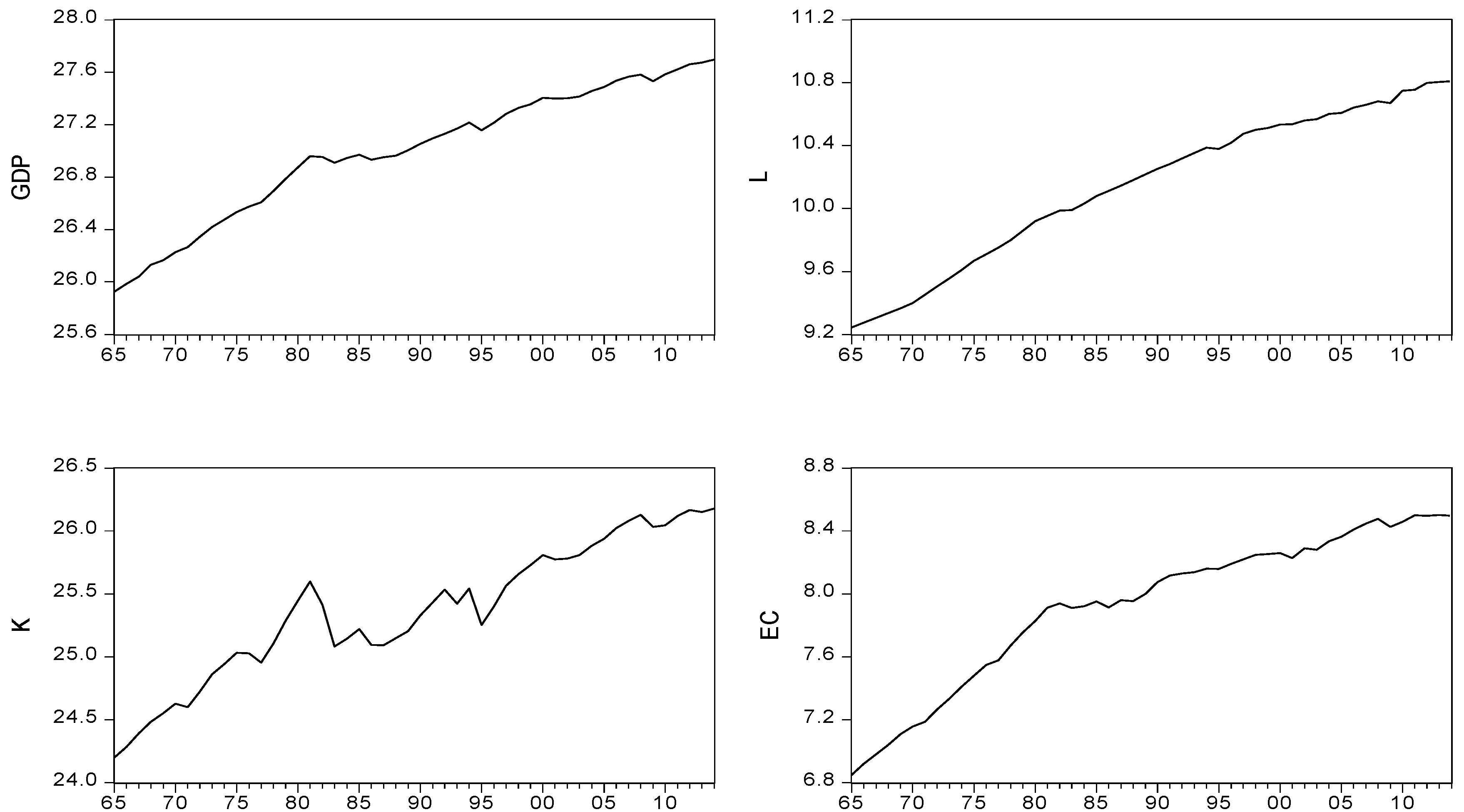
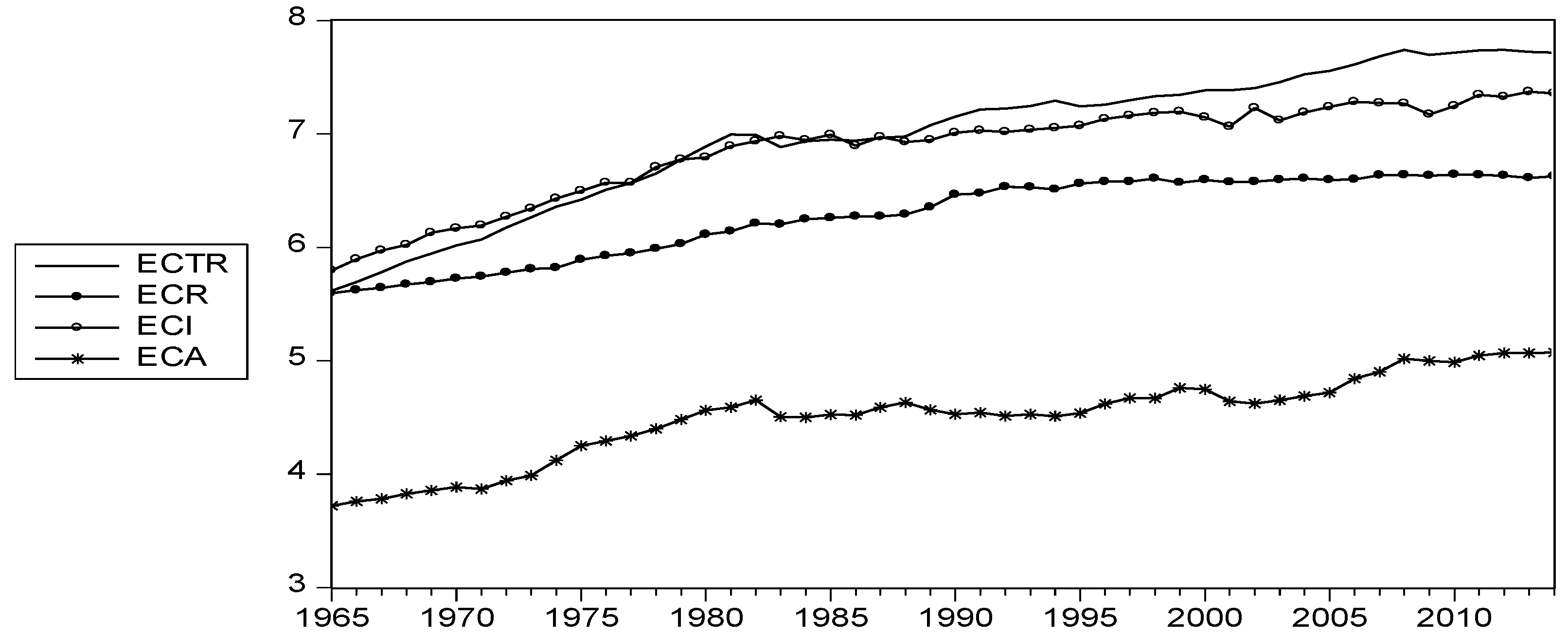
3. Data
4. Results
5. Conclusions and Policy Implications
Acknowledgments
Author Contributions
Conflicts of Interest
Appendix A

| Variable | Deterministic Parameters | ADF Test | PP Test |
|---|---|---|---|
| GDP K L EC ECR ECTR ECI ECA First differences ∆GDP ∆K ∆L ∆EC ∆ECR ∆ECTR ∆ECI ∆ECA | CT CT CT CT CT CT CT CT - - C C C C C C C C | −2.255 −2.826 −0.242 −1.706 0.238 −1.946 −2.348 −1.755 - - −5.054 * −6.139 * −6.049 * −4.908 * −5.963 * −4.084 * −8.191 * −5.252 * | −2.112 −2.900 −0.101 −1.694 0.318 −1.768 −2.440 −1.962 - - −5.054 * −6.188 * −6.210 * −5.013 * −6.160 * −4.062 * −8.066 * −5.249 * |
| From | To | Statistic | Dummy Variables |
|---|---|---|---|
| K L EC GDP L EC GDP K EC GDP K L | GDP GDP GDP K K K L L L EC EC EC | 2.84 *** 0.15 4.61 * 9.32 * 2.99 *** 1.46 6.52 * 5.55 * 15.42 * 0.35 0.91 4.56 ** | D83, D95, D09 D83, D95, D09 D83, D95, D09 D823, D86, D95 D823, D86, D95 D823, D86, D95 D83, D09 D83, D09 D83, D09 D83, D09 D83, D09 D83, D09 |
| From | To | Statistic | Control Variables |
|---|---|---|---|
| ECTR GDP ECR GDP ECI GDP ECA GDP | GDP ECTR GDP ECR GDP ECI GDP ECA | 1.32 0.33 1.13 3.73 ** 0.52 5.32 * 1.32 0.87 | K, L,D95, D09 K, L, D823, D09 K, L, D83, D95 K, L,D83, D90 K, L, D83, D95 K, L, D09, D2001 K, L, D83, D95, D09 K, L, D83 |
References
- Kraft, J.; Kraft, A. On the relationship between energy GNP. J. Energy Dev. 1978, 3, 401–403. [Google Scholar]
- Payne, J. A survey of the electricity consumption-growth literature. Appl. Energy 2010, 87, 723–731. [Google Scholar] [CrossRef]
- Bélaïd, F.; Abderrahmani, F. Electricity consumption and economic growth in Algeria: A multivariate causality analysis in the presence of structural change. Energy Policy 2013, 55, 286–295. [Google Scholar] [CrossRef]
- International Energy Agency (IEA). Energy and Air Pollution. World Energy Outlook Special Report. 2016. Available online: https://www.iea.org/ (accessed on 5 October 2016).
- Apergis, N.; Payne, J.E. A dynamic panel study of economic development and electricity consumption-growth nexus. Energy Econ. 2011, 33, 770–781. [Google Scholar] [CrossRef]
- Ciarreta, A.; Zarraga, A. Electricity consumption and economic growth in Spain. Appl. Econ. Lett. 2010, 17, 1417–1421. [Google Scholar] [CrossRef]
- Costantini, V.; Martini, C. The causality between energy consumption and economic growth: A multi-sectoral analysis using non-stationary cointegrated panel data. Energy Econ. 2010, 32, 591–603. [Google Scholar] [CrossRef]
- Destek, M.A.; Aslan, A. Renewable and non-renewable energy consumption and economic growth in emerging economies: Evidence from bootstrap panel causality. Renew. Energy 2017, 111, 757–763. [Google Scholar] [CrossRef]
- Eggoh, J.C.; Bangake, C.; Rault, C. Energy consumption and economic growth revisited in African countries. Energy Policy 2011, 39, 7408–7421. [Google Scholar] [CrossRef]
- Kumar, R.R.; Stauvermann, P.J.; Loganathan, N.; Kumar, R.D. Exploring the role of energy, trade and financial development in exploring economic growth in South Africa: A revisit. Renew. Sustain. Energy Rev. 2015, 52, 1300–1311. [Google Scholar] [CrossRef]
- Lee, C.C.; Chang, C.P. Structural breaks energy consumption, and economic growth revisited: Evidence from Taiwan. Energy Econ. 2005, 27, 857–872. [Google Scholar] [CrossRef]
- Mirza, F.M.; Kanwal, A. Energy consumption, carbon emissions and economic growth in Pakistan: Dynamic causality analysis. Renew. Sustain. Energy Rev. 2017, 72, 1233–1240. [Google Scholar] [CrossRef]
- Ozturk, I.; Acaravci, A. The long-run and causal analysis of energy, growth, openness and financial development on carbon emissions in Turkey. Energy Econ. 2013, 36, 262–267. [Google Scholar] [CrossRef]
- Rafindadi, A.A. Does the need for economic growth influence energy consumption and CO2 emissions in Nigeria? Evidence from the innovation accounting test. Renew. Sustain. Energy Rev. 2016, 62, 1209–1225. [Google Scholar] [CrossRef]
- Rafindadi, A.A.; Ozturk, I. Effects of financial development, economic growth and trade on electricity consumption: Evidence from post-Fukushina Japan. Renew. Sustain. Energy Rev. 2016, 54, 1073–1084. [Google Scholar] [CrossRef]
- Tang, C.F.; Shahbaz, M.; Arouri, M. Re-investigating the electricity consumption and economic growth nexus in Portugal. Energy Policy 2013, 62, 1515–1521. [Google Scholar] [CrossRef]
- Wolde-Rufael, Y. Electricity consumption and economic growth in transition countries: A revisit using bootstrap panel Granger causality analysis. Energy Econ. 2014, 44, 325–330. [Google Scholar] [CrossRef]
- Lean, H.H.; Smyth, R. Disaggregated energy demand by fuel type and economic growth in Malaysia. Appl. Energy 2014, 132, 168–177. [Google Scholar] [CrossRef]
- Liddle, B.; Lung, S. Revisiting energy consumption and GDP causality: Importance of a priori hypothesis testing, disaggregated data and heterogeneous panels. Appl. Energy 2015, 142, 44–55. [Google Scholar] [CrossRef]
- Rahman, M.d.S.; Noman, A.H.M.d.; Shahari, F. Does economic growth in Malaysia depend on disaggregate energy? Renew. Sustain. Energy Rev. 2017, 78, 640–647. [Google Scholar] [CrossRef]
- Tsani, S. Energy consumption and economic growth: A causality analysis for Greece. Energy Econ. 2010, 32, 582–590. [Google Scholar] [CrossRef]
- Zhang, W.; Yang, S. The influence of energy consumption of China on its real GDP from aggregated and disaggregated viewpoints. Energy Policy 2013, 57, 76–81. [Google Scholar] [CrossRef]
- Pablo-Romero, M.P.; Sánchez-Braza, A. Productive energy use and economic growth: Energy, physical and human capital relationships. Energy Econ. 2015, 49, 420–429. [Google Scholar] [CrossRef]
- Ayres, R.; Voudouris, V. The economic growth enigma: Capital, labour and useful energy? Energy Policy 2014, 64, 16–28. [Google Scholar] [CrossRef]
- Shen, K.; Whalley, J. Capital–labor–energy substitution in nested CES production functions for China. In The Economies of China and India Cooperation and Conflict; World Scientific: Singapore, 2017; Volume 2, pp. 15–27. [Google Scholar]
- Pablo-Romero, M.P.; Cruz, L.; Barata, E. Testing the transport energy-environmental Kuznets curve hypothesis in the EU27 countries. Energy Econ. 2017, 62, 257–269. [Google Scholar] [CrossRef]
- Chai, J.; Lu, Q.-Y.; Wang, S.-Y.; Lai, K.K. Analysis of road transportation energy consumption demand in China. Transp. Res. Part D 2016, 48, 112–124. [Google Scholar] [CrossRef]
- Chiou-Wei, S.Z.; Chen, C.-F.; Zhu, Z. Economic growth and energy consumption revisited—Evidence from linear and nonlinear Granger causality. Energy Econ. 2008, 30, 3063–3076. [Google Scholar] [CrossRef]
- Secretary of Energy. Estrategia Nacional de Energía 2013–2027. 2015. Available online: http://www.energia.gob.mx/res/PE_y_DT/pub/2013/ENE_2013-2027 (accessed on 13 March 2015).
- Cheng, B.S. Energy Consumption and Economic Growth in Brazil, Mexico and Venezuela: A Time Series Analysis. Appl. Econ. Lett. 1997, 4, 671–674. [Google Scholar] [CrossRef]
- Galindo, L.M.; Sánchez, L. El consumo de energía y la economía mexicana: Un análisis empírico con VAR. Econ. Mex. Nueva Época 2005, 0, 271–298. [Google Scholar]
- Bozoklu, S.; Yilanci, V. Energy consumption and economic growth for selected OECD countries: Further evidence from the Granger causality test in the frecuency domain. Energy Policy 2013, 63, 877–881. [Google Scholar] [CrossRef]
- Yıldırım, E.; Sukruoglu, D.; Aslan, A. Energy consumption and economic growth in the next 11 countries: The boostrapped autoregressive metric causality approach. Energy Econ. 2014, 44, 14–21. [Google Scholar] [CrossRef]
- Meng, M.; Lee, L.; Payne, J.E. RALS-LM unit root test with trend breaks and non-normal errors: Application to the Prebisch-Singer hypothesis. Stud. Nonlinear Dyn. Econ. 2017, 21, 31–45. [Google Scholar] [CrossRef]
- Pesaran, M.H.; Shin, Y.; Smith, R. Bounds testing approaches to the analysis of level relationships. J. Appl. Econ. 2001, 16, 289–326. [Google Scholar] [CrossRef]
- Bai, Z.; Wong, W.K.; Zhang, B. Multivariate linear and nonlinear causality tests. Math. Comput. Simul. 2010, 81, 5–17. [Google Scholar] [CrossRef]
- Stern, D.I. A multivariate cointegration analysis of the role of energy in the US macroeconomy. Energy Econ. 2000, 22, 267–283. [Google Scholar] [CrossRef]
- Dickey, D.A.; Fuller, W.A. Likelihood Ratio Tests for Autoregressive Time Series with a Unit Root. Econometrica 1981, 49, 1057–1072. [Google Scholar] [CrossRef]
- Phillips, P.C.B.; Perron, P. Testing for a Unit Roots in a Time Series Regression. Biometrika 1988, 75, 335–346. [Google Scholar] [CrossRef]
- Lee, J.; Strazicich, M. Minimum Lagrange Multiplier unit root test with two structural breaks. Rev. Econ. Stat. 2003, 85, 1082–1089. Available online: http://www.jstor.org/stable/3211829 (accessed on 25 January 2015). [CrossRef]
- Lee, J.; Strazicich, M. Minimum LM Unit Root Test with One Structural Breaks; Manuscript; Department of Economics, Appalachian State University: Boone, NC, USA, 2004; pp. 1–16. [Google Scholar]
- Lee, J.; Strazicich, M.; Meng, M. Two-step LM unit root tests with trend-breaks. J. Stat. Econ. Methods 2012, 1, 81–107. Available online: http://www.scienpress.com/Upload/JSEM/Vol%201_2_8.pdf (accessed on 25 January 2015).
- Payne, J.; Vizek, M.; Lee, J. Stochastic convergence in per capita fossil consumption in U.S. states. Energy Econ. 2017, 62, 382–395. [Google Scholar] [CrossRef]
- Narayan, P.K. The saving and investment nexus for China: Evidence from cointegration test. Appl. Econ. 2005, 37, 1979–1990. [Google Scholar] [CrossRef]
- Granger, C.W.J. Investigating causal relations by econometrics models and cross spectral methods. Econometrica 1969, 37, 424–438. [Google Scholar] [CrossRef]
- Toda, H.Y.; Yamamoto, T. Statistical inference in vector autoregressions with possibly integrated processes. J. Econ. 1995, 66, 225–250. [Google Scholar] [CrossRef]
- Granger, C.W.J. Some recent development in a concept of causality. J. Econ. 1988, 39, 199–211. [Google Scholar] [CrossRef]
- Hiemstra, C.; Jones, J.D. Testing for linear and nonlinear Granger causality in the stock price-volume relation. J. Financ. 1994, 49, 1639–1664. [Google Scholar] [CrossRef]
- World Bank. Available online: http://databank.bancomundial.org/data (accessed on 13 March 2016).
- Sadorsky, P. Trade and energy consumption in the Middle East. Energy Econ. 2011, 33, 739–749. [Google Scholar] [CrossRef]
- Wolde-Rufael, Y. Energy consumption and economic growth: The experience of African countries revisited. Energy Econ. 2009, 31, 217–224. [Google Scholar] [CrossRef]
- The Conference Board Total Economy Database. Available online: http://www.conference-board.org/data/economydatabase/ (accessed on 13 March 2015).
- Ruiz, P. Evolución y Determinantes del Tipo de Cambio en México; Documento de Trabajo, Universidad Nacional Autónoma de México: Ciudad de México, México, 1997; pp. 1–39. [Google Scholar]


| Variables | GDP | EC | ECTR | ECR | ECI | ECA |
|---|---|---|---|---|---|---|
| GDP | 1 | - | - | - | - | - |
| EC | 0.995 | 1 | - | - | - | - |
| ECTR | 0.996 | 0.998 | 1 | - | - | - |
| ECR | 0.975 | 0.981 | 0.976 | 1 | - | - |
| ECI | 0.979 | 0.992 | 0.985 | 0.965 | 1 | - |
| ECA | 0.967 | 0.969 | 0.971 | 0.917 | 0.964 | 1 |
| Variable | Model | Structural Break | LM Statistic | Lag Length | Structural Break | RALS-LM | Lag Length | |
|---|---|---|---|---|---|---|---|---|
| GDP | Model C | 1984 | −3.57 | 1 | 1983 | −3.70 ** | 0.99 | 0 |
| K | Model C | 1985 | −4.57 ** | 2 | 1982 | −4.73 * | 0.91 | 2 |
| L | Model C | 1991 | −3.26 | 0 | 1992 | −3.02 *** | 0.56 | 1 |
| EC | Model C | 1978 | −4.72 ** | 2 | 1982 | −6.91 * | 0.98 | 0 |
| ECR | Model C | 1992 | −3.83 | 2 | 1997 | −1.95 | 0.81 | 2 |
| ECTR | Model C | 1977 | −5.18 * | 4 | 1980 | −2.38 | 0.81 | 0 |
| ECI | Model C | 1981 | −5.57 * | 0 | 1982 | −6.91 * | 0.65 | 0 |
| ECA | Model C | 1985 | −2.81 | 1 | 1981 | −2.39 | 0.91 | 1 |
| First differences | ||||||||
| ∆GDP | Model A | 1982 | −6.63 * | 0 | 1982 | −7.44 * | 0.63 | 0 |
| ∆K | Model A | 1982 | −6.78 * | 0 | 1982 | −8.30 * | 0.58 | 0 |
| ∆L | Model A | 2007 | −8.25 * | 0 | 1971 | −6.69 * | 0.80 | 0 |
| ∆EC | Model A | 1982 | −7.00 * | 0 | 1982 | −6.52 * | 0.98 | 0 |
| ∆ECR | Model A | 1992 | −7.17 * | 0 | 1991 | −8.45 * | 0.78 | 0 |
| ∆ECTR | Model A | 1982 | −5.09 * | 0 | 1982 | −4.97 * | 0.90 | 0 |
| ∆ECI | Model A | 2010 | −9.07 * | 0 | 1987 | −9.39 * | 0.80 | 0 |
| ∆ECA | Model A | 1980 | −5.76 * | 0 | 1982 | −4.23 * | 0.85 | 0 |
| Variable | Model | Structural Breaks | LM Statistic | Lag Length | Structural Break | RALS-LM | Lag Length | |
|---|---|---|---|---|---|---|---|---|
| GDP | Model C | 1984/1998 | −5.11 *** | 2 | 1981/1990 | −6.27* | 0.98 | 0 |
| K | Model C | 1976/1985 | −5.86 * | 2 | 1980/1984 | −4.23 * | 0.71 | 0 |
| L | Model C | 1977/1995 | −4.33 | 0 | 1980/1993 | −8.80 * | 0.63 | 0 |
| EC | Model C | 1979/1988 | −5.97 * | 4 | 1980/2000 | −7.37 * | 0.97 | 0 |
| ECR | Model C | 1978/1996 | −6.00 * | 3 | 1978/1994 | −7.26 * | 0.79 | 1 |
| ECTR | Model C | 1978/1987 | −5.64 ** | 4 | 1969/1982 | −4.95 * | 0.58 | 0 |
| ECI | Model C | 1979/2001 | −6.17 * | 2 | 1982/990 | −7.20 * | 0.86 | 0 |
| ECA | Model C | 1977/2002 | −4.82 | 3 | 1981/1985 | −4.26 ** | 0.97 | 1 |
| First differences | ||||||||
| ∆GDP | Model A | 1982/1996 | −6.85 * | 0 | ||||
| ∆K | Model A | 1982/1987 | −7.32 * | 0 | ||||
| ∆L | Model A | 1980/1997 | −5.21 * | 0 | ||||
| ∆EC | Model A | 1981/1989 | −8.10 * | 0 | ||||
| ∆ECR | Model A | 1987/1992 | −8.03 * | 0 | ||||
| ∆ECTR | Model A | 1982/1986 | −5.79 * | 0 | ||||
| ∆ECI | Model A | 1995/2010 | −9.92 * | 0 | ||||
| ∆ECA | Model A | 1980/2002 | −5.91 * | 0 |
| ADRL Model | F-Test |
|---|---|
| F(GDP|K, L, EC, D86, D95, D09) | 6.34 ** |
| F(K|GDP, L, EC, D823, D86, D95) | 3.14 |
| F(L|GDP, K, EC, D95, D09) | 7.69 * |
| F(EC|GDP, K, L, D823, D86, D09) | 10.67 * |
| ADRL Model | F-Test |
|---|---|
| F(GDP|K, L, ECTR, D86, D95, D09) | 6.16 ** |
| F(ECTR|K, L, GDP, D823, D95, D09) F(GDP|K, L, ECI, D95) F(ECI|K, L, GDP, D86, D09, D01) F(GDP|K, L, ECR, D95) F(ECR|K, L, GDP, D90) | 4.10 *** 5.73 ** 5.61 ** 3.39 5.96 ** |
| F(GDP|K, L, ECA, D95) | 4.49 ** |
| F(ECA|K, L, GDP, D73, D83, D09) | 8.32 * |
| Explanatory Variables | ∆GDP | Dependent Variables ∆K | ∆L | ∆EC |
|---|---|---|---|---|
| ∆GDP | - | 5.33 ** | 3.02 *** | 1.20 |
| ∆K | 7.46 * | - | 1.53 | 1.39 |
| ∆L | 1.03 | 2.34 | - | 4.34 ** |
| ∆EC | 1.88 | 2.26 | 7.43 * | - |
| ECT-1 Dummy | −0.60 ** D83, D95, D09 | 0.07 D823, D86, D95 | −0.03 D83, D09 | 0.22 D83, D09 |
| Diag. tests JB Normal LM test White test Ramsey test | - 2.43 2.07 8.23 0.44 | - 2.83 1.72 3.53 0.15 | - 3.24 0.56 9.44 1.83 | - 2.04 0.39 6.33 1.00 |
| Explanatory Variables | ∆GDP | ∆ECTR | ∆GDP | Dependent Variables ∆ECI | ∆GDP | ∆ECR | ∆GDP | ∆ECA |
|---|---|---|---|---|---|---|---|---|
| ∆GDP | - | 0.46 | - | 2.51 *** | - | 3.30 *** | - | 1.99 |
| ∆K | 6.28 * | 0.29 | 9.61 * | 1.11 | 13.34 * | 1.44 | 2.81 *** | 1.83 |
| ∆L | 0.47 | 0.22 | 0.000 | 0.62 | 0.00 | 7.40 * | 0.96 | 0.04 |
| ∆ECTR ∆ECI | 0.86 - | - - | - 2.75 | - - | - - | - - | - - | - - |
| ∆ECR ∆ECA ECT-1 Dummy | - - −0.66 ** D95,D09 | - - 0.39 D823,D09 | - - −0.82 ** D83,D95 | - - 0.77 D01, D09 | 1.39 - 0.66 ** D83,D95 | - - 0.06 D83,D90 | - 1.39 −0.21 D83,D95,D09 | - - 0.38 D83 |
| Diag. Tests JB Normal LM test White test Ramsey test | - 1.72 5.07 20.48 0.15 | - 1.79 2.28 3.78 0.76 | - 2.06 1.84 3.81 0.13 | - 1.86 4.20 5.85 0.07 | - 1.42 1.13 4.10 0.03 | - 1.54 1.03 9.81 1.13 | - 1.25 3.89 8.50 0.47 | - 0.16 0.84 3.56 0.07 |
© 2018 by the authors. Licensee MDPI, Basel, Switzerland. This article is an open access article distributed under the terms and conditions of the Creative Commons Attribution (CC BY) license (http://creativecommons.org/licenses/by/4.0/).
Share and Cite
Gómez, M.; Ciarreta, A.; Zarraga, A. Linear and Nonlinear Causality between Energy Consumption and Economic Growth: The Case of Mexico 1965–2014. Energies 2018, 11, 784. https://doi.org/10.3390/en11040784
Gómez M, Ciarreta A, Zarraga A. Linear and Nonlinear Causality between Energy Consumption and Economic Growth: The Case of Mexico 1965–2014. Energies. 2018; 11(4):784. https://doi.org/10.3390/en11040784
Chicago/Turabian StyleGómez, Mario, Aitor Ciarreta, and Ainhoa Zarraga. 2018. "Linear and Nonlinear Causality between Energy Consumption and Economic Growth: The Case of Mexico 1965–2014" Energies 11, no. 4: 784. https://doi.org/10.3390/en11040784
APA StyleGómez, M., Ciarreta, A., & Zarraga, A. (2018). Linear and Nonlinear Causality between Energy Consumption and Economic Growth: The Case of Mexico 1965–2014. Energies, 11(4), 784. https://doi.org/10.3390/en11040784