Multi-Objective Optimal Energy Management for the Integrated Electrical and Natural Gas Network with Combined Cooling, Heat and Power Plants

Abstract

This paper proposes a multi-objective optimal energy management framework for the integrated electrical and natural gas network (IEGN) with combined cooling, heat, and power (CCHP) plants. Various energy conversion devices that are installed in the CCHP plant provide redundant generation options and energy pathways, which could be optimally chosen and shifted with given objectives, while meeting the multi-energy (ME) demands. However, this flexible energy dispatch manners may frequently change the energy distribution in the IEGN and challenge their mutual accommodation. In particular, the linepack reserve in the natural gas network, which supports the ramping capabilities of both the gas turbines and the flexible energy dispatch of the gas-dependent ME devices, is highly influenced. Without enough linepack reserve, not only will the flexible operation of the CCHP plants be hindered, but also the gas turbines will be prevented from balancing the supply and the demand in the electrical network, thus threatens the safety of the IEGN. Owing to this, the linepack reserve is modelled and jointly considered in the proposed energy management framework. The multi-objective optimization model that is proposed in this paper could simultaneously promote the economic benefits, safety, and efficiency of the IEGN, and Elitist Non-dominated Sorting Genetic algorithm II is used to solve it. At last, case studies demonstrate the effectiveness of the proposed method.

1. Introduction

With the development of the multi-energy system, more and more different energy sectors are coupled together, such as the integrated electrical network and natural gas network (IEGN). Meanwhile, the distributed multi-generation solutions, especially the combined cooling, heat, and power (CCHP), have proliferated. CCHP plants facilitate the interaction between the electricity and gas networks, and promote the efficiency and environmental friendliness of the IEGN as a whole [1,2,3]. However, the increasingly more frequent interactions that are caused by the CCHP plants may challenge the coordination and mutual accommodation of the IEGN [2,3]. In particular, it greatly influences the linepack reserve in the natural gas network [4,5], which plays an important role in supporting the gas turbines to ramp up and down, and to serve the balancing needs in the electrical network, and thus may harm the safe operation of the IEGN [6,7,8].

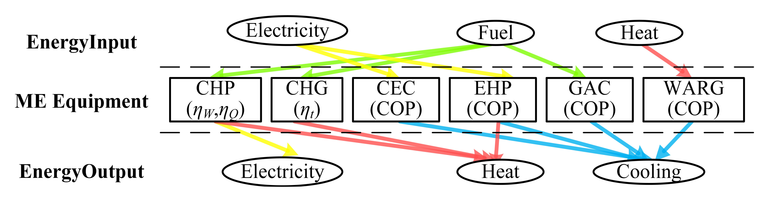
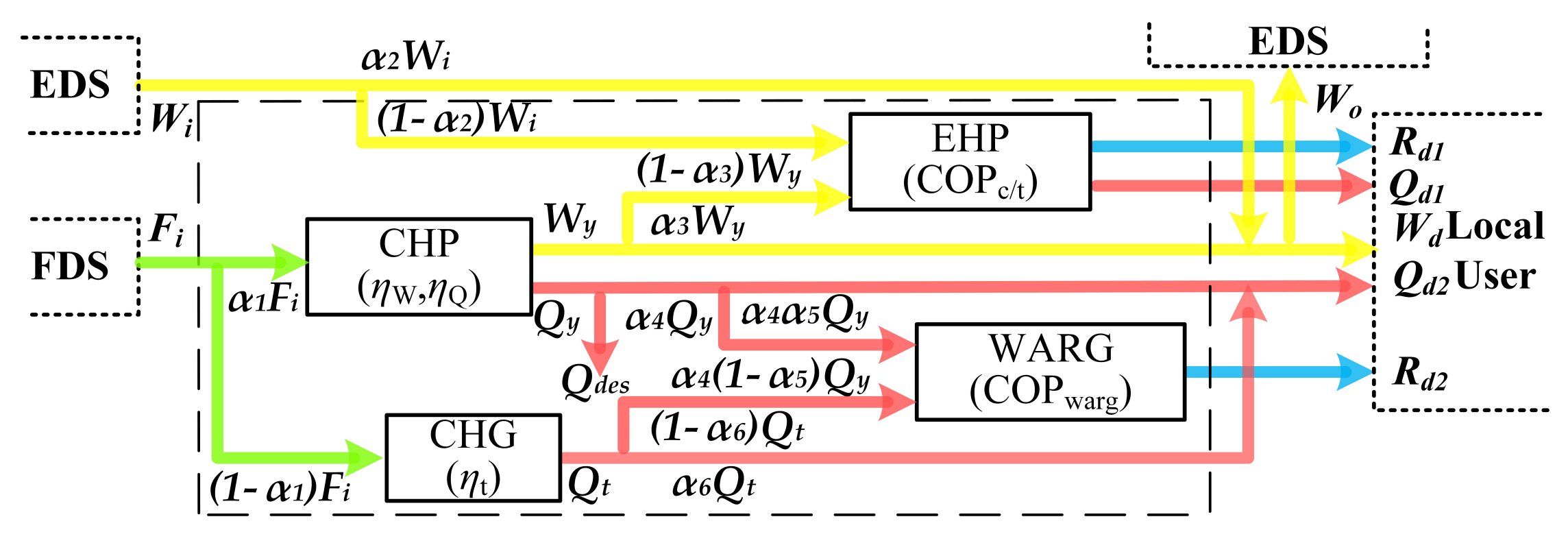
The CCHP plant, whereby various energy conversion devices are installed to supply multi-energy (ME) demands (electricity, heat, and cooling) from multiple input energy sources (natural gas, electricity, and so on), provides redundant energy generation options and energy pathways inside. For example, heat could be produced with electricity (in electrical heaters), or fuel (in combustion groups); cooling could be generated from electricity (in electric chillers) or heat (in absorption chillers) [9,10,11]. Hence, various generation combinations can be used to supply the ME demands, which will cause different energy exchanges with the interconnected energy networks. According to the specific generation combination, the ME demand can be supplied through electricity alone, or through natural gas alone, or both. The generation combinations can be optimally chosen, and shift with purposes, while meeting the ME demands [11]. This flexible energy dispatch shift of the CCHP plants provides extra flexibility to the IEGN and demonstrates the significant potential in optimizing the operation performance of the IEGN. Traditional energy management studies regarding the CCHP plants only consider limited types of ME devices in the modelling process, however the flexibility that is brought by the redundant generation options, especially the internal energy dispatch shift, has been rarely considered in the energy management of the CCHP plants so far.

Nonetheless, this flexible energy dispatch manners of the CCHP plant will frequently change the energy distribution both in the electrical network and the natural gas network, which will change the linepack reserves in the gas network. At the same time, not only the normal gas turbines, the flexible energy dispatch of many ME devices, such as the combined cycle gas turbine (CCGT), require enough linepack reserves as well. Therefore, the linepack reserve should be jointly considered in the energy management of the CCHP plants in order to promote both the efficiency and the safety of the IEGN. If not, not only the flexible energy dispatch of the CCHP plant may be hindered from realization, but also the gas turbines may be prevented from balancing the demands in a power system, which may undermine the operating reserve adequacy and threatens the safety of the IEGN [4,5]. Besides, as the development of the IEGN, the electrical networks are more and more dependent on the fast-response flexibility provided by the gas turbines and the linepack reserve. For instance, it is more and more used by system operators to balance the stochastic renewable energy sources [12]. Many studies regarding the linepack reserve are mainly about securing the safe operation of the natural gas network, as far as the authors know, the linepack reserve has not been literally considered in the energy management of the IEGN with CCHP plants yet, although its impact on the IEGN management is huge. Therefore, lineack reserve should be an integral part of the energy management of the IEGN.

The modelling analysis of the CCHP plants [9,10,11], and the IEGN [13,14,15], has been addressed in many publications, based on which many energy management methods are proposed [16,17,18]. Based on the efficiency matrices and energy dispatch factors (EDF), Pierluigi Mancarella [11] discusses the flexible internal energy dispatch of the CCHP plant and investigates its potential in providing real time demand response services. Ref. [4,19,20,21,22] introduces the linepack reserve in the natural gas network. Ref. [20,21] define the linepack reserve as a kind of buffer that could be used without safety problem, and [4,22] highlights its importance as a “balancing tool” in serving the balancing needs of the IEGN. Ref. [19] evaluates the flexibility of the IEGN by measuring the flexibility that gas turbines can provide by employing the linepack reserve in the natural gas network. Based on the steady state models of the electrical network and the natural gas network, and the security constraints in both of the networks, ref. [16,17,18,23] present several optimization models for the IEGN energy management. Ref. [16] studies the combined economic dispatch of the IEGN. The mathematical model is formulated as an optimization problem where the objective function is to minimize the integrated gas-electricity system operation cost, and the constraints are the power system and natural gas pipeline equations and capacities. The evolutionary algorithm is applied to solve the optimization problem. A multi-objective optimization for the combined gas and electricity network expansion planning was presented in [23]. The objectives are to minimize both the investment cost and production cost of the combined system while taking into account the N-1 network security criterion. The constraints of the optimization model include the operation and security constraints of IEGN and equality constraint that links the two networks, and the Elitist Non-dominated Sorting Genetic Algorithm II (NSGAII) is used to solve the optimization problem. Ref. [17] incorporates the energy management of a CCHP plant into the combined economic dispatch model of the IEGN with the concept of ‘energy hub’ to minimize the total generation cost. Besides the constraints of the traditional optimal dispatch optimization model, the constraints on energy hubs are included, and the numerical methods are used to solve the optimization problem. Ref. [18] establishes a multi-objective model for a microgrid with CCHP plant to optimize the daily operation cost, the daily environment cost, and the primary energy rate. The constraints of energy balances and devices output power are considered, and the particle swarm optimization algorithm is used to solve the model. Despite the energy management of CCHP plants are considered in [17,18], only one single CCHP plant and limited types of ME devices are discussed, which brought concerns: (1) The types of the considered ME devices are too few to model the flexible and shiftable energy dispatch of the CCHP plants, and to investigate its impact on the linepack reserve of the IEGN. Besides, the coordination of CCHP plants with different configurations are not considered, which impacts the operation performance of the IEGN and should be part of the energy management of the CCHP plants (2) The purposes of prior-at researches on the IEGN energy management are mainly about economy, rarely having the security of both networks considered. In particular, the linepack reserve has not been considered in the energy management of the IEGN with CCHP plants.

In light of the above issues, this paper develops an optimal energy management framework for an IEGN with multiple CCHP plants, which jointly considers the lineapck reserve in the IEGN, aiming at meeting the ME demands in a most economic, efficient, and secure way. At first, several typical ME devices are introduced and modelled with the efficiency matrices and EDFs, and based on which, the energy management of the CCHP plants, including the flexible energy dispatch, is integrated into the energy management of the entire IEGN. Then, the linepack reserve of the IEGN is modelled, and considered as an objective in the energy management framework to better secure the safety of the IEGN. When considering that the proposed optimization model is mathematically a multi-objective, mixed integer non-linear model, which cannot be easily solved with classical mathematical techniques, the NSGAII [24] is applied to find reasonable tradeoffs. The main contributions of this paper are threefold:

• The energy management of the CCHP plants, including the flexible energy dispatch is modelled, and its impact on the operation performance of the IEGN, especially the linepack reserve, is investigated and considered in the proposed energy management framework.
• For the efficiency and security of the IEGN, linepack reserve in the natural gas network is modeled and is jointly considered in the energy management framework.
• A multi-objective optimization model for the energy management of the IEGN is developed to simultaneously promote the profits, linepack reserve, and efficiency of the IEGN.

The rest of this paper is organized as follows. Section 2 presents the modelling of the CCHP plants, and the linepack reserve is modelled in Section 3. In Section 4, a multi-objective optimization model for the energy management of IEGN is proposed and tested on an IEGN case in Section 5. Finally, this paper is concluded in Section 6.

2. Modelling of the CCHP Plants

2.1. Typical CCHP Device

In order to illustrate the flexibility provided by the CCHP plant, several typical ME devices shown in Figure 1 are considered in this paper: 1. Combined heat and power (CHP) units. Electrical efficiency η_W and heat efficiency η_Q are used to describe the ratio of electric power output W and heat power output Q to the fuel thermal energy input F, respectively; 2. A CHP unit is typically sided by an auxiliary combustion heat generator group (CHG). Heat efficiency η_t is used to describe the ratio of heat power output to the fuel thermal energy input; 3. Compression Electric Chiller (CEC). Cooling power R for air conditioning or industrial purposes is conventionally generated by a CEC, whose compressor is driven by electricity; 4. Electrical heat pumps (EHP). EHP is an electrically driven bimodal machine that can serve both as a heater and a chiller; 5. Absorption chiller (WARG–Water Absorption/Adsorption Refrigeration Group). Cooling can be provided through a WARG [25] that produces cooling from a heat supply; 6. There are ME devices with other energy transforming mechanisms, which are less widespread, such as gas absorption chiller (GAC) and engine driven chiller (EDC), which are powered by mechanical compressors [25].

2.2. Energy Input and Output Model of CCHP Plants

Figure 2 shows a typical CCHP plant. It receives electricity supply from the Electrical Distribution System (EDS) and fuel from the Fuel Distribution System (FDS). As drawn in Figure 2, four ME devices and many energy pathways can be used to supply the ME demands. Electricity can be both bought from and sold to markets through the EDS. Heat demands can be met by exploiting CHP, CHG, and the EHP (heating mode). The cooling demand can be met by using the WARG or/and the EHP (cooling mode). Electricity can be drawn from the EDS and/or produced by the CHP (and can be sold back as well). In order to illustrate the internal energy dispatch, EDF is introduced [11]. Elements in an EDF vector are defined as the relative energy dispatch at flow splitting points (bifurcations) in order to supply a different ME device, whose number is determined by the configuration of the CCHP plant. In particular, with reference to the notation of Figure 2, the EDF is defined as in (1). In (1), α₁ is the relative fuel dispatch of the fuel input between CHP and CHG; α₂ is the relative electricity dispatch of the electricity input between EHP and local consumer; α₃ is the relative electricity dispatch of the electricity that is produced by the CHP between EHP and local consumer; α₄ denotes the ratio of heat produced by CHP that is not deserted; α₅ is the relative electricity dispatch of the heat produced by CHP between WARG and local consumer; and, α₆ is the relative electricity dispatch of the heat that is produced by CHG between WARG and local consumer. The EHP operation in heating mode or in cooling mode is not mutually exclusive, and μ ∈ [0,1] denotes the proportion of electricity used for the heat production in all the electricity supply of the EHP

$$\alpha ={\left[{\alpha }_1,{\alpha }_2,{\alpha }_3,{\alpha }_4,{\alpha }_5,{\alpha }_6,\mu \right]}^T$$

(1)

If we use $E_o={\left[F_o,W_o,Q_o,R_o\right]}^T$ and $E_i={\left[F_i,W_i,Q_i,R_i\right]}^T$ denote the output and input energy vectors, respectively, the mapping between them can be described with an efficiency matrix H as in (2). F_o, W_o, Q_o, R_o denote the fuel output, electricity output, heat output, and cooling power output, respectively; F_i, W_i, Q_i, R_i denote the fuel input, electricity input, heat input, and cooling power input, respectively. Each element in H relates one particular input to a certain output with relevant performance indicator, as defined in

Table 1. ME device and performance indicators.

ME Device	Performance Indicator
CHP	ηW = W/F; ηQ = Q/F
CHG	ηt = Q/F
CEC, EHP (cooling mode)	COPc = R/W
WARG	COPc = R/Q
GAC, EDC	COPc = R/F
EHP (heating mode)	COPt = Q/W

[9,10,11]. η_FF, η_FW, η_FQ, η_FR denotes the ratio of fuel output and fuel input, electricity input, heat input, and cooling power input, respectively; η_WF, η_WW, η_WQ, η_WR denotes the ratio of electricity output and fuel input, electricity input, heat input, and cooling power input, respectively; η_QF, η_QW, η_QQ, η_QR denotes the ratio of heat output and fuel input, electricity input, heat input, and cooling power input, respectively; η_RF, η_RW, η_RQ, η_RR denotes the ratio of cooling power output and fuel input, electricity input, heat input, and cooling power input. respectively.

$$\begin{array}{c}{E}_o=H\cdot E_i\\ H=\left[\begin{array}{cccc}{\eta }_{FF}& {\eta }_{FW}& {\eta }_{FQ}& {\eta }_{FR}\\ {\eta }_{WF}& {\eta }_{WW}& {\eta }_{WQ}& {\eta }_{WR}\\ {\eta }_{QF}& {\eta }_{QW}& {\eta }_{QQ}& {\eta }_{QR}\\ {\eta }_{RF}& {\eta }_{RW}& {\eta }_{RQ}& {\eta }_{RR}\end{array}\right]\end{array}$$

(2)

The energy input and output relation of the CCHP plant in Figure 2 is achieved as (3) and (4). E_d is the local energy demand and E_ex is the energy exchange with external energy distribution networks.

$$\begin{array}{c}H=\left(\begin{array}{cccc}0& 0& 0& 0\\ {\alpha }_3{\alpha }_1{\eta }_W& {\alpha }_2& 0& 0\\ {\eta }_{QF}& \mu CO{P}_t\left(1-{\alpha }_2\right)& 0& 0\\ {\eta }_{RF}& \left(1-\mu \right)CO{P}_c\left(1-{\alpha }_2\right)& 0& 0\end{array}\right)\\ {\eta }_{QF}={\alpha }_5\left(1-{\alpha }_1\right){\eta }_t+{\alpha }_4{\alpha }_1{\eta }_Q+\mu CO{P}_t\left(1-{\alpha }_3\right){\eta }_W{\alpha }_1\\ {\eta }_{RF}=CO{P}_c\left(1-{\alpha }_3\right){\alpha }_1{\eta }_W+\left(1-\mu \right)CO{P}_{w\arg }\cdot \left[\left(1-{\alpha }_5\right)\left(1-{\alpha }_1\right){\eta }_t+{\alpha }_4{\alpha }_1{\eta }_Q\right]\end{array}$$

(3)

$$E_o=H\cdot E_i=E_d+E_{ex}$$

(4)

With (1) and (2), the internal energy dispatch of the concerned CCHP and its corresponding energy exchanges with other energy sectors could be represented through a matrix formulism, and the flexible energy dispatch shift of the CCHP could be modelled with the shift of EDFs. This makes it easy to integrate the energy management of the CCHP in the optimization model of the entire IEGN.

2.3. Energy Saving Indicator of IEGN

In [10], the energy saving performance of a CCHP plant is evaluated with the trigeneration primary energy saving (TPES) indicator, as shown in (5). In (5), F_tri is the thermal energy of the primary energy input; W_tri is the net electricity output; Q_tri is the net heat output; R_tri is the cooling power output; F^SP is the total fuel thermal energy input required for the separate production of the same energy demand; and, ${\eta }_e^{\mathrm{SP}}$, ${\eta }_t^{\mathrm{SP}}$, and COP^SP are the separate production reference efficiencies for, respectively, electricity, heat, and cooling power.

$$TPES=\frac{F^{\mathrm{SP}}-F_{tri}}{F^{\mathrm{SP}}}=1-\frac{F_{tri}}{W_{tri}/{\eta }_e^{\mathrm{SP}}+Q_{tri}/{\eta }_t^{\mathrm{SP}}+R_{tri}/{\eta }_e^{\mathrm{SP}}\cdot CO{P}^{\mathrm{SP}}}$$

(5)

In this evaluation process, no matter how complex are the energy flows within a CCHP plant, only the actual input and output matter. If the IEGN is seen as a CCHP plant, W_tri, Q_tri, and R_tri are replaced with the total electric, heat, and cooling output of the IEGN, W, Q, and R, and F_tri with the total primary energy consumption F, the primary energy saving performance (PESP) of the IEGN could be evaluated with (6).

$$PESP=\frac{F^{\mathrm{SP}}-F}{F^{\mathrm{SP}}}=1-\frac{F}{W/{\eta }_e^{\mathrm{SP}}+Q/{\eta }_t^{\mathrm{SP}}+R/{\eta }_e^{\mathrm{SP}}\cdot CO{P}^{\mathrm{SP}}}$$

(6)

3. Linepack Reserve of IEGN

In this section, the linepack reserve of the natural gas network is modelled at first. Then, the roles it plays in providing balancing services to the IEGN, and securing the safe interaction between the electrical networks and natural gas networks are discussed.

3.1. Linepack Reserve of Natural Gas Network

Assume that the volume of a pipe π is s_π. The inlet and outlet nodal pressures are p₁ and p₂, respectively (p₁ > p₂). The gas flow F_π is given by (7), where c_π is the pipeline constant that depends on the properties of the pipeline (length, diameter, and the absolute rugosity) and on the gas composition [26].

$$sign\left(F_{\mathsf{\pi }}\right)F_{\mathsf{\pi }}^2=c_{\mathsf{\pi }}^2\left(p_1^2-p_2^2\right)$$

(7)

Pipeline linepack is defined as the quantity of gas in a pipeline at a given time. With p_NTP denoting the pressure at normal temperature and pressure (NTP), z denoting the compressibility factor, the linepack of π is given by (8).

$$L_{\pi }=\frac{z{s}_{\pi }}{p_{\mathrm{NTP}}}\frac{2}{3}\left(p_1+p_2-\frac{p_1{p}_2}{p_1+p_2}\right)$$

(8)

Linepack plays multiple roles in the operation of a natural gas network, including maintaining minimum offtake pressures, flow characteristics, and allowing for variations in the supply and demand, which may not be balanced instantaneously [4]. As the natural gas flow is related to the difference of the quadratic pressures at both ends of the pipeline, the network operator can change the nodal pressures within a certain range, while ensuring the expected natural gas transport. Linepack reserve is defined as the amount of natural gas that can be managed flexibly by controlling the operation pressure levels between a safe pressure band.

For a pipeline π, assume that its daily maximum natural gas condition is composed of maximum power demand $\overline{D_P}$ and non-power demand $\overline{D_N}$. Then, its minimum and maximum linepack can be determined, when $\overline{D_P}+\overline{D_N}$ are, respectively, transported at its minimum and maximum pressure level. Assume that the inlet nodal pressure p₁ is equal to the maximum pressure $\overline{p}$, then according to (7), the outlet nodal pressure and the maximum linepack of π are defined, as in (9) and (10).

$$p_2=\sqrt{p_1^2-{\left(\overline{D_{\mathrm{P}}}+\overline{D_{\mathrm{N}}}\right)}^2/c^2}$$

(9)

$$\overline{L_{\mathsf{\pi }}}=\frac{Z\cdot V}{p_{\mathrm{NTP}}}\frac{2}{3}(\overline{p}+\sqrt{{\overline{p}}^2-{\left(\overline{D_{\mathrm{P}}}+\overline{D_{\mathrm{N}}}\right)}^2/c^2}-\frac{\overline{p}\sqrt{{\overline{p}}^2-{\left(\overline{D_{\mathrm{P}}}+\overline{D_{\mathrm{N}}}\right)}^2/c^2}}{\overline{p}+\sqrt{{\overline{p}}^2-{\left(\overline{D_{\mathrm{P}}}+\overline{D_{\mathrm{N}}}\right)}^2/c^2}})$$

(10)

Similarly, assume that the outlet nodal pressure p₂ is equal to the minimum pressure $\underset{\_}{p}$, then the inlet nodal pressure and the minimum linepack of π are defined as in (11) and (12).

$$p_1=\sqrt{p_2^2+{\left(\overline{D_{\mathrm{P}}}+\overline{D_{\mathrm{N}}}\right)}^2/c^2}$$

(11)

$$\underset{\_}{L_{\mathsf{\pi }}}=\frac{Z\cdot V}{p_{\mathrm{NTP}}}\frac{2}{3}(\underset{\_}{p}+\sqrt{{\underset{\_}{p}}^2+{\left(\overline{D_{\mathrm{P}}}+\overline{D_{\mathrm{N}}}\right)}^2/c^2}-\frac{\underset{\_}{p}\sqrt{{\underset{\_}{p}}^2+{\left(\overline{D_{\mathrm{P}}}+\overline{D_{\mathrm{N}}}\right)}^2/c^2}}{\underset{\_}{p}+\sqrt{{\underset{\_}{p}}^2+{\left(\overline{D_{\mathrm{P}}}+\overline{D_{\mathrm{N}}}\right)}^2/c^2}})$$

(12)

Combine (7)–(12), (13), and (14) can be achieved,

$$\overline{L{r}_{\mathsf{\pi }}}=\overline{L_{\mathsf{\pi }}}-L_{\mathsf{\pi }},\underset{\_}{L{r}_{\mathsf{\pi }}}=L_{\mathsf{\pi }}-\underset{\_}{L_{\mathsf{\pi }}}$$

(13)

$$L{r}_{\mathsf{\pi }}=\overline{L_{\mathsf{\pi }}}-\underset{\_}{L_{\mathsf{\pi }}}$$

(14)

In (13), upward linepack reserve $\overline{L{r}_{\mathsf{\pi }}}$ is defined as the difference between the maximum linepack and the present linepack; the downward linepack reserve $\underset{\_}{L{r}_{\mathsf{\pi }}}$ is defined as the difference between the present linepack and the minimum linepack. $\overline{L{r}_{\mathsf{\pi }}}$ and $\underset{\_}{L{r}_{\mathsf{\pi }}}$, respectively, reflect the amount of natural gas that could be stored in and withdrawn from π. In (14), $L{r}_{\mathsf{\pi }}$ denotes the linepack reserve in π, which reflects the capacity of the natural gas that can be flexibly managed.

As the pipeline types and the natural gas flow that each pipeline transports vary, when the linepack reserve of a natural gas network is assessed, each pipeline must be calculated individually. Then, the sum of the linepack reserve of each pipeline are the linepack reserve of the natural gas network. For a natural gas network z with pipeline set Ω_pipe, the upward linepack reserve $\overline{L{r}_z}\left(t_0\right)$, downward reserve $\underset{\_}{L{r}_z}\left(t_0\right)$ and linepack reserve $L{r}_z\left(t_0\right)$ are as shown in (15) and (16),

$$\overline{L{r}_z}\left(t_0\right)={\displaystyle \sum _{i\in {\mathsf{\Omega }}_{\mathrm{pipe}}}\overline{L_i}\left(t_0\right)-L_i\left(t_0\right)},\underset{\_}{L{r}_z}\left(t_0\right)={\displaystyle \sum _{i\in {\mathsf{\Omega }}_{\mathrm{pipe}}}{L}_i\left(t_0\right)-\underset{\_}{L_i}\left(t_0\right)}$$

(15)

$$L{r}_z\left(t_0\right)={\displaystyle \sum _{i\in {\mathsf{\Omega }}_{\mathrm{pipe}}}\overline{L_i}\left(t_0\right)-\underset{\_}{L_i}\left(t_0\right)}$$

(16)

3.2. Flexibility Assessment of IEGN

When the natural gas supply-load mismatches occur, which are usually caused by the fluctuations either on the gas supply or the gas load, the linepack reserve will automatically be employed to mitigate the supply-load gap, as shown in Figure 3. Owing to the technical constraints, natural gas contractors can only change its supply, as scheduled on hour basis [4,27,28,29]. On the load side, the fluctuation on non-power gas load, mainly thermal load, is usually minor and negligible. As the interaction between the electrical networks and natural gas networks increases, more and more supply-load mismatches are caused by the fluctuations on the power generating load, which are usually resulting from a supply-load imbalance in the electrical sector. In the following analysis, the role linepack reserve plays in serving the balancing needs of the electrical network are mainly focused. Generally, as long as the natural gas-fired generating units can withdraw enough linepack reserve in time, the power flow fluctuation could be mitigated. This involves concerns both on the time window and the ramping capability of the natural gas-fired generating units.

The timeframe over which the linepack reserve may be withdrawn for flexibility requirements is defined as the linepack reserve utilization period, T. T is dependent on the gas network as well as its scheduling capability. For larger gas networks, where changes to supply flows take longer to filtrate through the network before reaching demand, a longer linepack reserve utilization period should be considered. Meanwhile, for gas networks that actively manage their operation, for example, through the use of compressor stations, shorter timeframes should be considered [19]. In Figure 3, when the previous T ends and a new T begins, not only the present linepack, but the maximum linepack and the minimum linepack should be recalculated based on the maximum natural gas flow in this period. Thus, the upward linepack reserve and the downward linepack reserve will be renewed.

The ramping capability of a gas turbine reflects its ability in employing linepack reserve, i.e., the ability in serving the balancing purposes in the electrical network. Assume that the concerned gas turbines have the same maximum outputs $\overline{P_{\mathrm{GT}}}\left(t\right)$, minimum outputs $\underset{\_}{P_{\mathrm{GT}}}\left(t_0\right)$, initial outputs $P_{\mathrm{GT}}\left(t_0\right)$, and ramping rate R_GT. Assume that it takes $t_{\mathrm{acc}}=(\overline{P_{\mathrm{GT}}}-P_{\mathrm{GT}}(t_0))/R_{\mathrm{GT}}$ to increase their outputs from $P_{\mathrm{GT}}\left(t_0\right)$ to $\overline{P_{\mathrm{GT}}}\left(t\right)$, $t_{\mathrm{dec}}=(P_{\mathrm{GT}}(t_0)-\underset{\_}{P_{\mathrm{GT}}})/R_{\mathrm{GT}}$ to decrease their outputs from $P_{\mathrm{GT}}\left(t_0\right)$ to $\underset{\_}{P_{\mathrm{GT}}}\left(t_0\right)$. If the linepack reserve capacity is infinite, $\overline{W_{\mathrm{GT}}}\left(t_0\right)$ and $\underset{\_}{W_{\mathrm{GT}}}\left(t_0\right)$ in (17) and (18) are the maximum output increment and maximum output decrement that the gas turbine could achieve in T with the employment of linepack reserve.

$$\overline{W_{\mathrm{GT}}}\left(t_0\right)=\{\begin{array}{ll}\frac{1}{2}{R}_{\mathrm{GT}}\cdot t_{\mathrm{acc}}^2+\left(\overline{P_{\mathrm{GT}}}-P_{\mathrm{GT}}\left(t_0\right)\right)\cdot \left(T-t_{\mathrm{acc}}\right),& t_{\mathrm{acc}}\le T\\ \frac{1}{2}{R}_{\mathrm{GT}}\cdot T^2,& t_{\mathrm{acc}}>T\end{array}$$

(17)

$$\underset{\_}{W_{\mathrm{GT}}}\left(t_0\right)=\{\begin{array}{ll}\frac{1}{2}{R}_{\mathrm{GT}}\cdot t_{\mathrm{dec}}^2+\left(P_{\mathrm{GT}}\left(t_0\right)-\underset{\_}{P_{\mathrm{GT}}}\right)\cdot \left(T-t_{\mathrm{dec}}\right),& t_{\mathrm{dec}}\le T\\ \frac{1}{2}{R}_{\mathrm{GT}}\cdot T^2,& t_{\mathrm{dec}}>T\end{array}$$

(18)

Assume that all of the gas turbines in z share the same efficiency η_z, and the heat value of the natural gas is denoted by q, the maximum capacity of the fast-response flexibility that gas-fired generating units can provide is derived as (19) and (20),

$$\overline{E_z}\left(t_0\right)=\min \left\{\underset{\_}{L{r}_z}\left(t_0\right)\cdot q\cdot {\eta }_z,\overline{W_{\mathrm{GT}}}\left(t_0\right)\right\}$$

(19)

$$\underset{\_}{E_z}\left(t_0\right)=\min \left\{\overline{L{r}_z}\left(t_0\right)\cdot q\cdot {\eta }_z,\underset{\_}{W_{\mathrm{GT}}}\left(t_0\right)\right\}$$

(20)

4. Optimization Model for the Energy Management

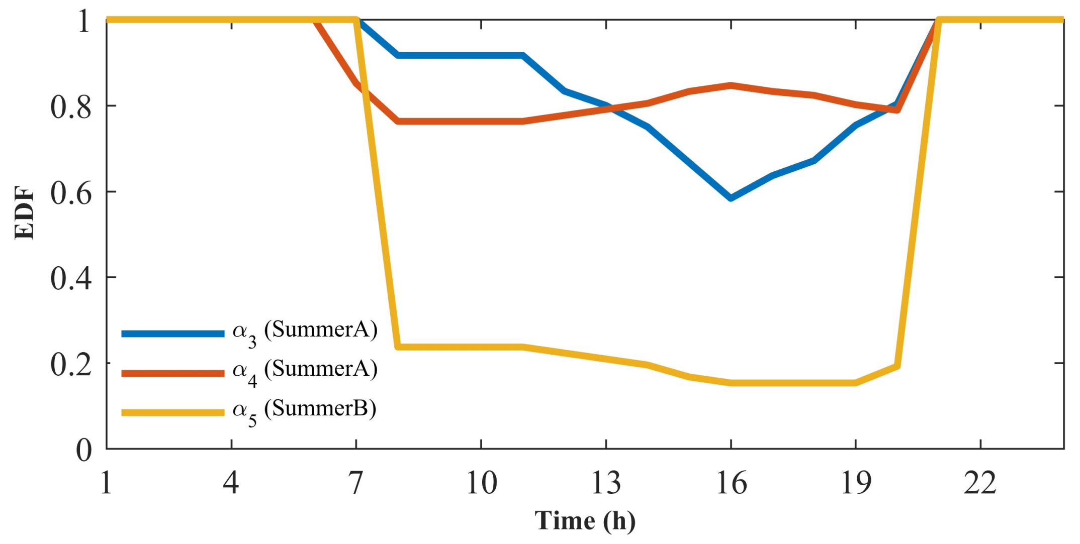
Based on the models that are developed above, a multi-objective optimization model is formulated in this section. The decision variables vector V is defined as in (21). In (21), p and G are the nodal pressure vector and natural gas input vector for the natural gas network, P_GT is the output vector for normal gas turbines, and α is the EDF vector for CCHP plants.

$$V={\left[\mathit{p},\mathit{G},{\mathit{P}}_{\mathrm{GT}},\mathit{\alpha }\right]}^T$$

(21)

The purpose of the proposed optimization model is to improve the profits, linepack reserve, and energy saving performance of the IEGN, simultaneously. So, the objective function comprises of three individual objectives, namely F₁, F₂, and F₃.

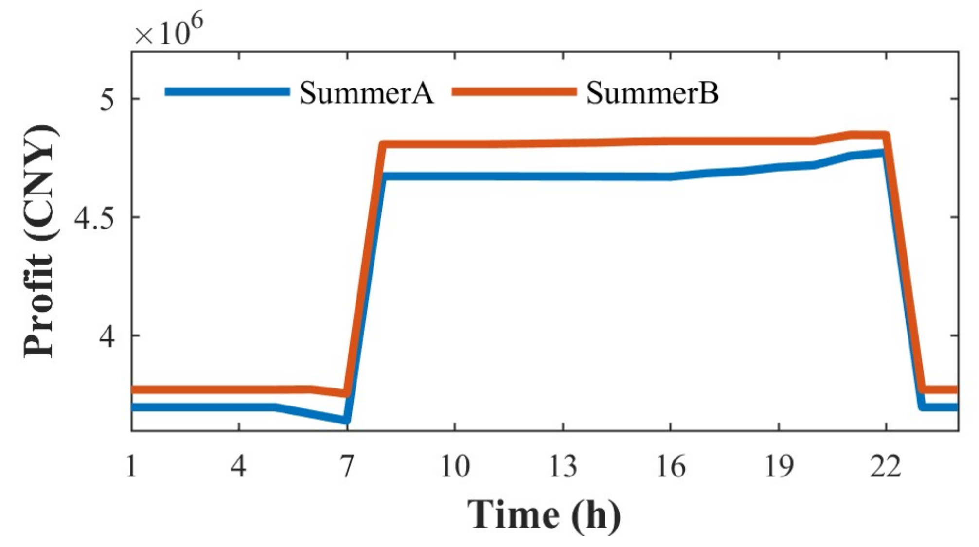
F₁ is modeled as the profits of the IEGN, which is the total revenue by selling electricity minus the generation cost.

$$\begin{array}{ll}{F}_1=& \max [{\displaystyle \sum _{i\in N}{\rho }_o^{\mathrm{EDS}}\cdot P_{l,i}}-{\displaystyle \sum _{j\in {\mathsf{\Omega }}_{\mathrm{CG}}}\left(a_j+b_j\cdot P_{\mathrm{CG},j}+c_j\cdot P_{\mathrm{CG},j}^2\right)}\\ & -{\displaystyle \sum _{k\in {\mathsf{\Omega }}_{\mathrm{GT}}}{\rho }_{\mathrm{GT}}^{\mathrm{FDS}}\left(P_{\mathrm{GT},k}/\left({\eta }_{\mathrm{GT},k}\cdot q\right)\right)}-{\displaystyle \sum _{m\in {\mathsf{\Omega }}_{\mathrm{CCHP}}}{\rho }_{\mathrm{CCHP}}^{\mathrm{FDS}}\cdot F_{\mathrm{CCHP},\mathrm{m}}}]\end{array}$$

(22)

In (22), Ω_CG, Ω_GT, and Ω_CCHP are the conventional generators set, gas-fired generators set and CCHP plants set, respectively; P_l,i is the electric load on the Bus i, P_CG,j is the output of conventional generator j, P_GT,k is the output of gas turbine k; a_j, b_j, and c_j are the consumption characteristic factors of generator j; ${\rho }_o^{\mathrm{EDS}}$ is the hourly selling price of electricity, ${\rho }_{\mathrm{GT}}^{\mathrm{FDS}}$ is the hourly fuel price for power generating; and, ${\rho }_{\mathrm{CCHP}}^{\mathrm{FDS}}$ is the hourly fuel price for heat and cooling power production.

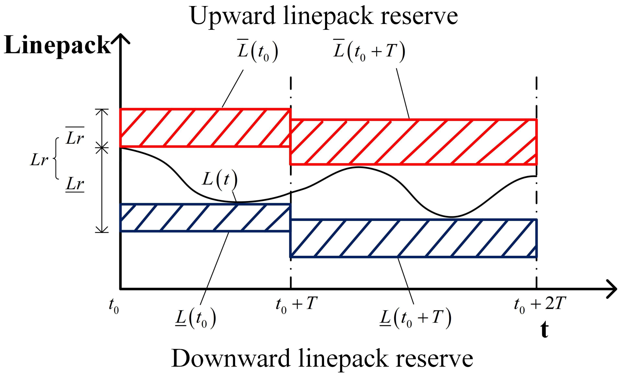
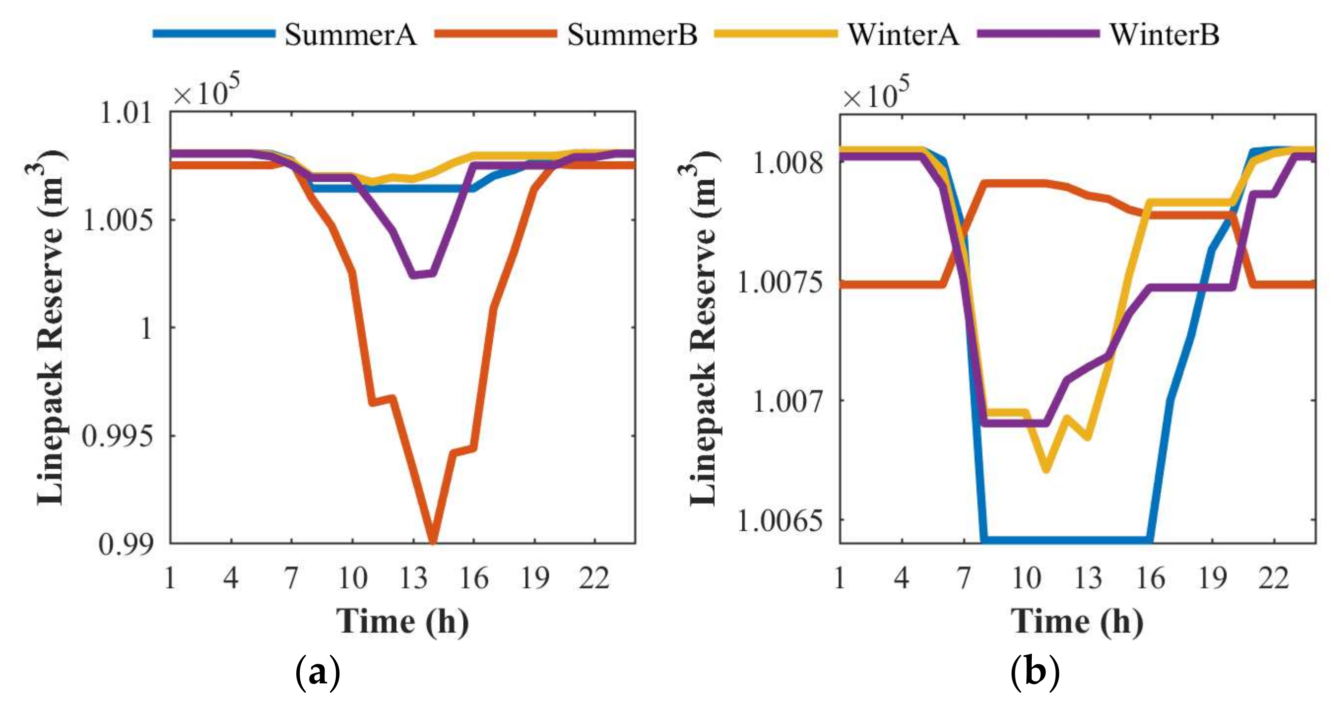
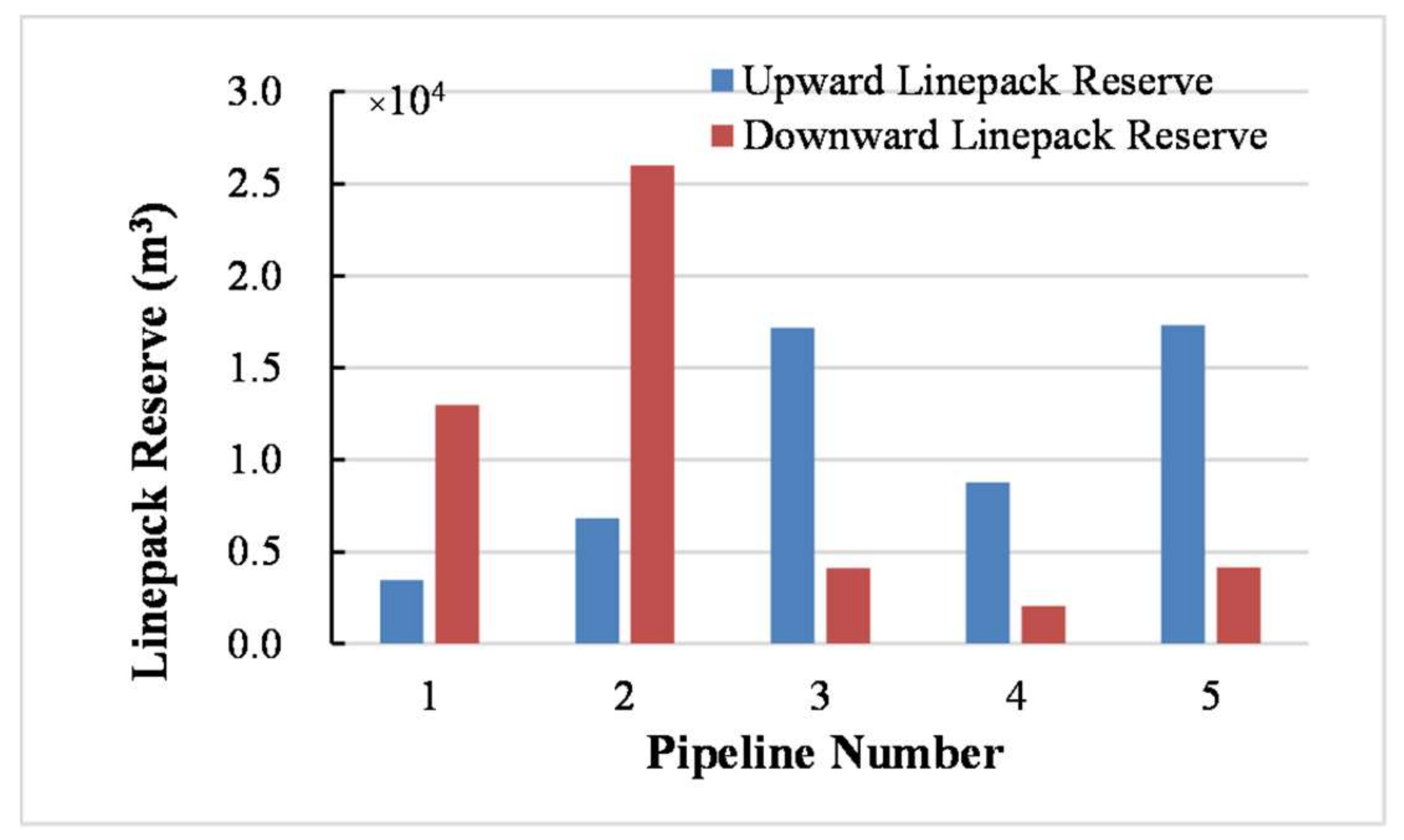
F₂ is modeled as the linepack reserve of the IEGN, as given by,

$$F_2=\max {\displaystyle \sum _{i\in {\mathsf{\Omega }}_{\mathrm{pipe}}}L{r}_i}$$

(23)

In (23), $L{r}_i$ is the linepack reserve of the pipeline i. The detailed calculation process is as shown in (7)–(16).

F₃ is modelled as the PESP of the IEGN assessed by the primary energy saving indicator, as shown in (24)–(26). W_CCHP,m, Q_CCHP,m, and R_CCHP,m are, respectively, the electricity, heat, and cooling output of the CCHP plant m.

$$F_3=\max \{1-\frac{F}{W/{\eta }_{\mathrm{e}}^{\mathrm{SP}}+Q/{\eta }_{\mathrm{t}}^{\mathrm{SP}}+R/{\eta }_{\mathrm{e}}^{\mathrm{SP}}\cdot CO{P}^{\mathrm{SP}}}\}$$

(24)

$$F={\displaystyle \sum _{j\in {\mathsf{\Omega }}_{\mathrm{CG}}}{P}_{\mathrm{CG},j}/{\eta }_{\mathrm{e}}^{\mathrm{SP}}}+{\displaystyle \sum _{k\in {\mathsf{\Omega }}_{\mathrm{GT}}}{P}_{\mathrm{GT},k}/{\eta }_{\mathrm{GT},k}}+{\displaystyle \sum _{m\in {\mathsf{\Omega }}_{\mathrm{ME}}}{F}_{\mathrm{CCHP},\mathrm{m}}}$$

(25)

$$\begin{array}{l}W={\displaystyle \sum _{j\in {\mathsf{\Omega }}_{\mathrm{CG}}}{P}_{\mathrm{CG},j}}+P_{\mathrm{GT},k}+{\displaystyle \sum _{m\in {\mathsf{\Omega }}_{\mathrm{CCHP}}}{W}_{\mathrm{CCHP},\mathrm{m}}}\\ Q={\displaystyle \sum _{m\in {\mathsf{\Omega }}_{\mathrm{CCHP}}}{Q}_{\mathrm{CCHP},\mathrm{m}}},R={\displaystyle \sum _{m\in {\mathsf{\Omega }}_{\mathrm{CCHP}}}{R}_{\mathrm{CCHP},\mathrm{m}}}\end{array}$$

(26)

The constraints of the proposed optimization model are composed of electrical network constraints, natural gas network constraints, ME devices constraints, and linepack reserve constraints.

$$\begin{array}{l}{P}_{Gi}-P_{Li}-U_i{\displaystyle \sum _{j=1}^n{U}_j\left(G_{ij}\cos {\theta }_{ij}+B_{ij}\sin {\theta }_{ij}\right)}=0\left(i,j\in {\mathsf{\Omega }}_{\mathrm{B}}\right)\\ Q_{Gi}-Q_{Li}-U_i{\displaystyle \sum _{j=1}^n{U}_j\left(G_{ij}\sin {\theta }_{ij}-B_{ij}\cos {\theta }_{ij}\right)}=0\left(i,j\in {\mathsf{\Omega }}_{\mathrm{B}}\right)\end{array}$$

(27)

$$\underset{\_}{P_{Gi}}\le P_{Gi}\le \overline{P_{Gi}},\underset{\_}{Q_{Gi}}\le Q_{Gi}\le \overline{Q_{Gi}}\left(i\in {\mathsf{\Omega }}_{\mathrm{G}}\right)$$

(28)

$$\begin{array}{l}\left|S_{ij}\right|\le \overline{S_{ij}}\left(i,j\in {\mathsf{\Omega }}_{\mathrm{B}}\right)\\ \underset{\_}{U_i}\le U_i\le \overline{U_i}\left(i\in {\mathsf{\Omega }}_{\mathrm{B}}\right)\end{array}$$

(29)

(27)–(29) Are electrical network constraints. (27) Represents the active and reactive power balance for each bus. (28) Represents the output limits of generators. (29) Represents the operational limits on the apparent power and the steady-state voltage magnitude. Ω_B and Ω_G denote the buses set and the generator buses set, respectively. P_Gi and Q_Gi denote the active and reactive power outputs, P_Li and Q_Li denote the active and reactive power loads, U_i denotes the voltage magnitude of Bus i and θ_ij denotes the voltage angle gap between Bus i and Bus j, G_ij and B_ij denote the real and imaginary parts of the ith row the jth column element in the nodal admittance matrix. S_ij denotes the apparent power between bus i and bus j.

$$S_i-D_i={\displaystyle \sum _{\begin{array}{l}j=1\\ j\ne i\end{array}}^n{F}_{ij}}\left(i,j\in {\mathsf{\Omega }}_{\mathrm{NG}}\right)$$

(30)

$$\mathrm{sign}\left(F_{ij}\right)F_{ij}^2=c_{ij}^2\left(p_i^2-p_j^2\right)\left(i,j\in {\mathsf{\Omega }}_{\mathrm{NG}}\right)$$

(31)

$$\left|F_{ij}\right|\le \overline{F_{ij}},\underset{\_}{p_i}\le p_i\le \overline{p_i}\left(i,j\in {\mathsf{\Omega }}_{\mathrm{NG}}\right)$$

(32)

(30)–(32) Are the natural gas network constraints. Ω_NG denotes the natural gas network nodes set. (30) Represents the natural gas flow balance for each node in the natural gas network. (31) Represents the pipeline natural gas flow function. S_i and D_i denote the natural gas injection and the natural gas load on Node i, F_ij denotes the natural gas flow between Node i and Node j, p_i and p_j are nodal pressures of Node i and Node j, respectively. c_ij is the pipeline constant. (32) Represents the operation limits on pipes and nodal pressure.

$$\underset{\_}{E_{o,x}}\le H_x\cdot E_{i,x}\le \overline{E_{o,x}}(x\in {\mathrm{CCHP}}_i,{\mathrm{CCHP}}_i\in {\mathsf{\Omega }}_{\mathrm{CCHP}})$$

(33)

$$H^{{\mathrm{CCHP}}_i}\cdot E_i^{{\mathrm{CCHP}}_i}=E_d^{{\mathrm{CCHP}}_i}+E_{ex}^{{\mathrm{CCHP}}_i}({\mathrm{CCHP}}_i\in {\mathsf{\Omega }}_{\mathrm{CCHP}})$$

(34)

(33) and (34) are the CCHP plants constraints. In (33), $\overline{E_{o,x}}$ and $\underset{\_}{E_{o,x}}$ are the maximum output and minimum output of ME device x in the CCHP plant CCHP_i. In (34), $E_i^{{\mathrm{CCHP}}_i}$ and $E_d^{{\mathrm{CCHP}}_i}$ are the energy input of CCHP_i and local ME demands, $E_{ex}^{{\mathrm{CCHP}}_i}$ is the energy exchange between CCHP_i and the external energy distribution networks.

$$\overline{E}\left(t_0\right)\ge {\displaystyle {\int }_{t_0}^{t_0+\mathrm{T}}F{S}_{\max }\left(t\right)-F{D}_{\min }\left(t\right)dt}$$

(35)

$$\underset{\_}{E}\left(t_0\right)\ge {\displaystyle {\int }_{t_0}^{t_0+\mathrm{T}}F{S}_{\min }\left(t\right)-F{D}_{\max }\left(t\right)dt}$$

(36)

(35) and (36) are constraints on the linepack reserve, which are conceived to guarantee the fluctuations that are caused by the forecasting errors either in the supply or the demand can be mitigated with the linepack reserve. [FS_max, FS_min] and [FD_max, FD_min] denote the forecasting output interval of power plants and the forecasting load interval.

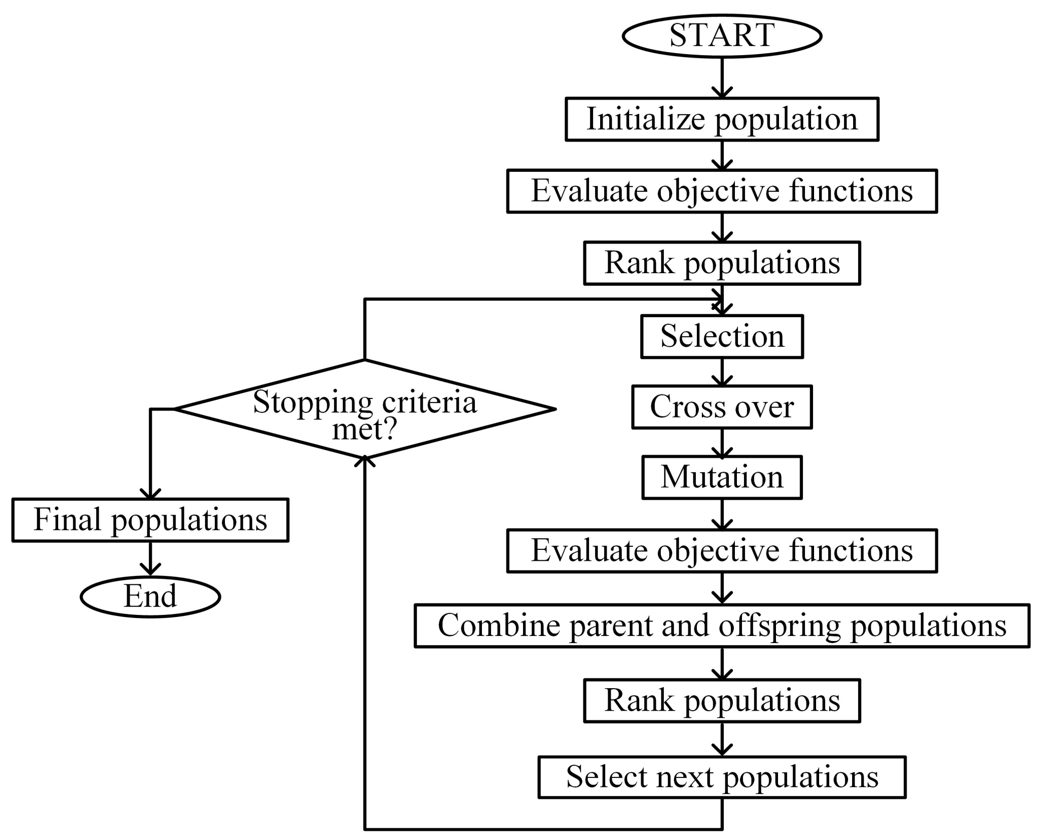
Mathematically, this is a multi-objective, mixed integer non-linear problem, which cannot be easily solved by classical mathematical techniques. To address this, NSGAII [22] is used. NSGAII is an improved version of NSGA based on Pareto optimal set, whose main loop is shown in Figure 4. It starts by initializing the population and assigning an appropriate rank based on the fast non-dominated sorting approach. Then, reproduction operators, such as tournament selection, recombination, and mutation are used to create the offspring population. Under the elitist-preserving strategy, next generation population is generated via the competition between parent and offspring populations. The excellent individuals in the present generation are added into the next generation. More details about NSGAII can be found in [24].

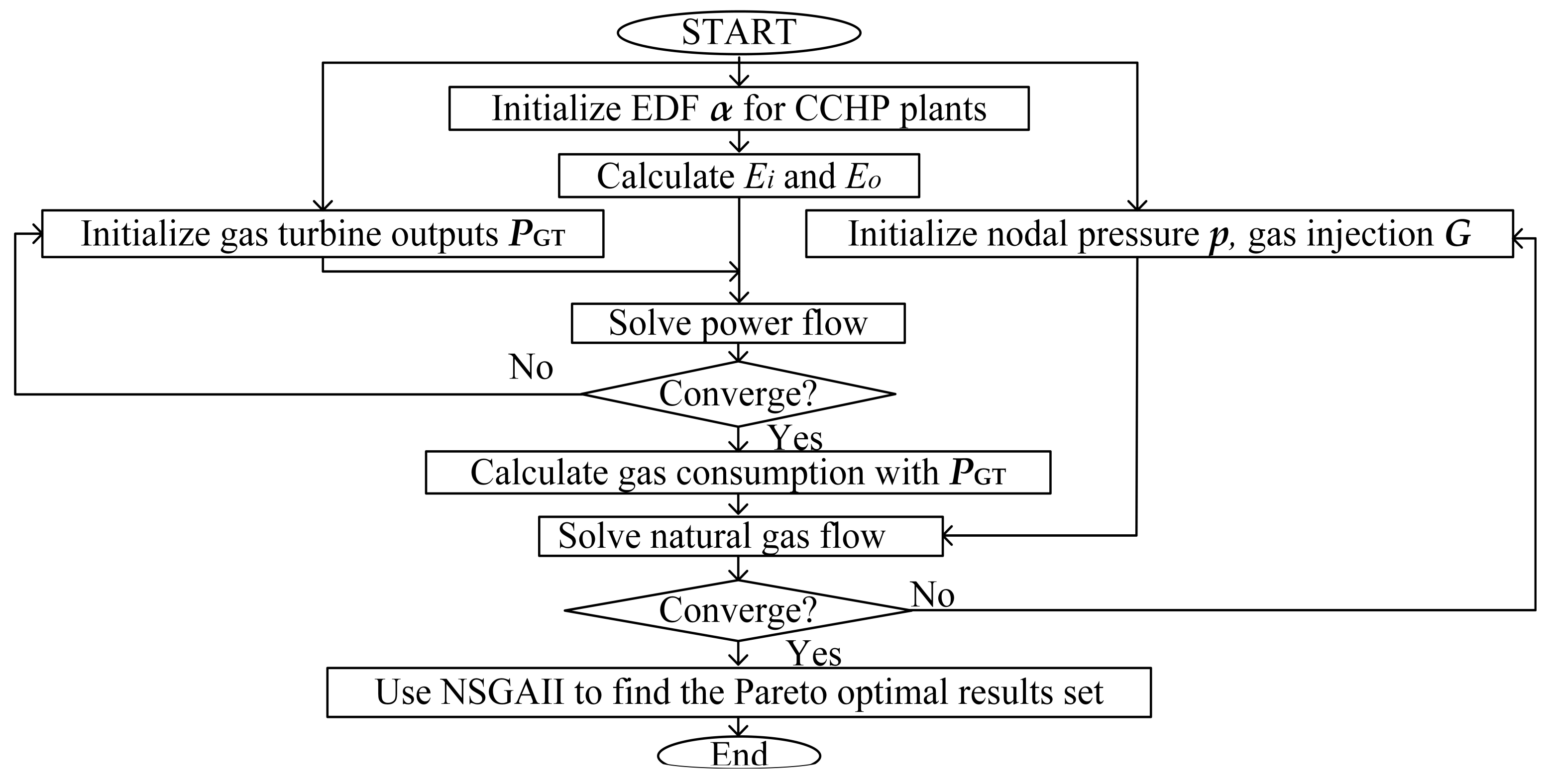
With the NSGAII algorithm, the whole computation process that is shown in Figure 5 could be summarized as follows.

Step 1: Initialize the outputs of normal gas-fired generator buses as P_GT, except the CCHP plants buses or the slack bus.

Step 2: Initialize EDF vectors for CCHP plants buses as α. Calculate electricity output W and natural gas thermal energy input F, according to the local ME demands.

Step 3: Solve the power flow of the electrical network. Calculate the natural gas demand of normal natural gas-dependent generating units for the calculation of the natural gas flow.

Step 4: Initialize the nodal pressure for all of the nodes in the natural gas network as p, the natural gas injection from natural gas sources as G. Solve the natural gas flow with natural gas demands that were calculated in the previous steps.

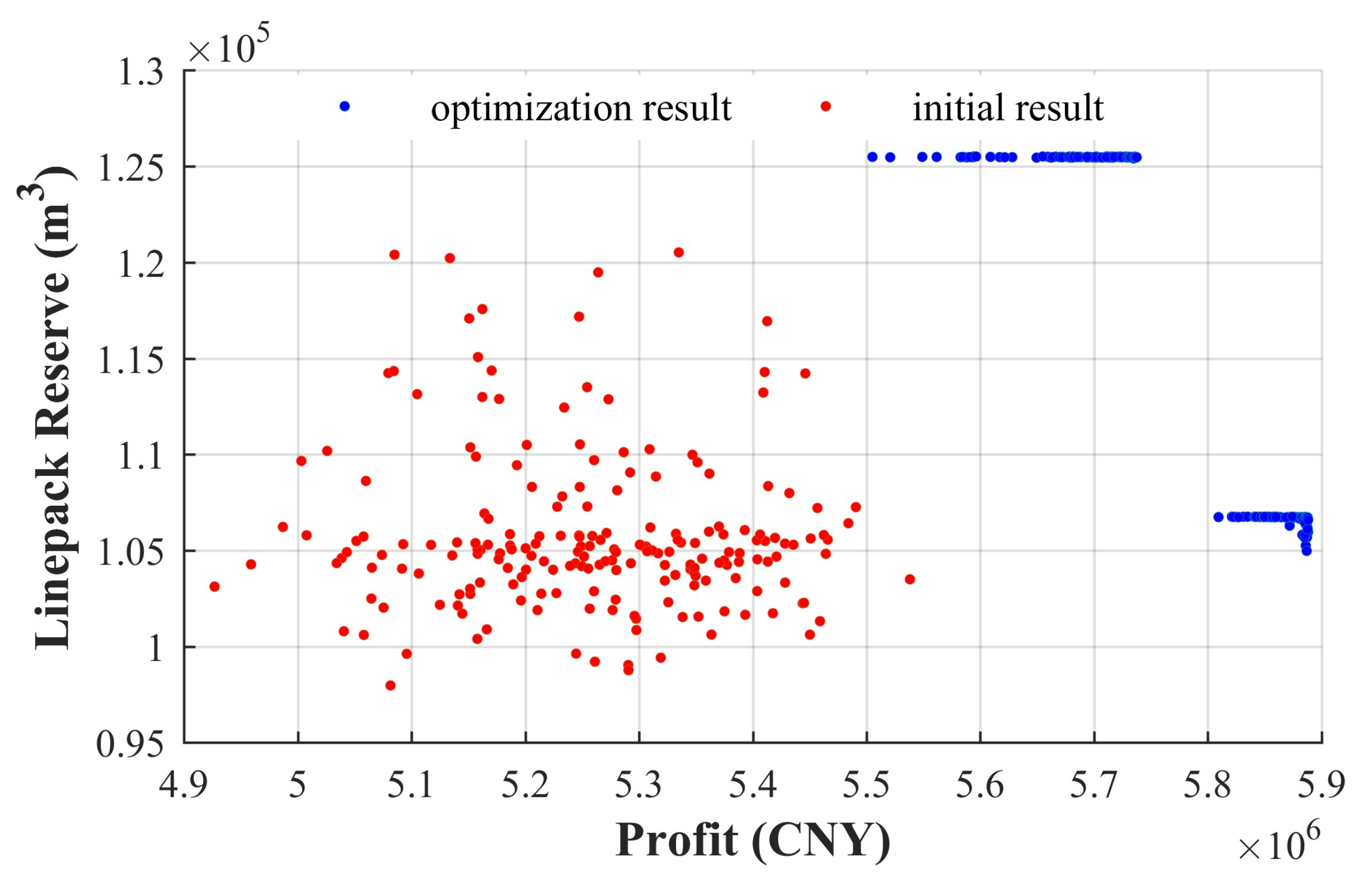
Step 5: NSGAII is employed to achieve the Pareto-optimal front set.

5. Case Study

Two cases are conceived and tested on an IEGN consisting of the IEEE 39-bus system (case39.m from MATPOWER 6.5) and a natural gas network, as illustrated in Figure 6. The green natural gas network on the right and the blue electrical network on the left are coupled via three natural gas-dependent plants. Bus 33, 35, and 37 are connected with Node 4, 2, and 3, respectively. Details of two normal natural gas-dependent plants are listed in

Table 2. Gas turbines in electrical network.

Bus Number	Efficiency	Capacity
35	η1 = 60%	508 MW
37	η2 = 45%	580 MW

. Detailed parameters of the pipelines in the natural gas network are listed in

Table 3. Pipeline parameters in natural gas network.

Pipeline	Length	Diameter	Max Pressure	Min Pressure
1–2	20 km	625 mm	0.4 MPa	0.2 MPa
2–3	20 km
2–4	40 km
3–4	40 km
1–4	40 km

. The linepack reserve utilization period T is set as 1 h. The natural gas price is 2.36 ¥/m³ for thermal and cooling power production, 2.51 ¥/m³ for electricity generation, and the selling price of electricity is 0.65 ¥/kW·h in 8:00–22:00 and 0.52 ¥/kW·h in other hours [30,31].

5.1. Case A

This case is conceived to illustrate the impacts of CCHP plants on the linepack reserve and the profits of the IEGN. Two different CCHP plants are alternately connected with the IEGN between Bus 33 and Node 4. The configurations of CCHP plant 1 and CCHP plant 2 are, respectively, illustrated in Figure 2 and Figure 7, and are listed in

Table 4. ME device in CCHP plant 1.

ME Device	Efficiency	Capacity
CHP	ηW = 36%	300 MW
	ηQ = 43%
CHG	${\eta }_t^{\mathrm{SP}}$ = 90%	650 MW
EHP	COP = 3.5	150 MW
WARG	COPWARG = 0.65	800 MW

and

Table 5. ME device in CCHP plant 2.

ME Device	Efficiency	Capacity
CHP	ηW = 36%	300 MW
	ηQ = 43%
CHG	${\eta }_t^{\mathrm{SP}}$ = 90%	650 MW
EHP	COP = 3.5	100 MW

. Figure 8 is the assigned hourly pattern for ME demands [32]. Two simple energy dispatch strategies are considered for illustration: A. electrical load following; B. thermal load following. When Strategy A is followed, CCHP plant will mainly rely on electricity-dependent ME devices, such as EHP; while, when Strategy B is followed, the natural gas-dependent ME devices, such as CHG, will be considered with priority.

In Figure 9, Figure 9a shows the linepack reserve of the IEGN when the CCHP plant 1 is online and Figure 9b shows the linepack reserve of the IEGN when CCHP plant 2 is online. From Figure 9, we may clearly see the impacts of the CCHP plant configuration, CCHP plant energy dispatch, and the ME demands on the linepack reserve of the IEGN. The differences between Figure 9a and Figure 9b are mainly resulted from the configuration difference of the two CCHP plants. In one single picture, no matter Figure 9a or Figure 9b, the differences among four linepack reserve profiles are caused by the different energy demands and energy dispatch. Generally, linepack reserves in Figure 9a have a larger fluctuating range than those in Figure 9b, which is because with one more gas-dependent ME equipment-WARG, CCHP plant 1 can exert more influences on the IEGN linepack reserve. When Strategy A is followed, no matter in summer or winter, the linepack reserve are nearly the same (see Figure 9a,b). Because the heat and cooling production mainly relies on EHP under Strategy A, the natural gas demands of the two CCHP plants are nearly the same. When Strategy B is followed, the cooling and heat production for CCHP plant 1 mainly depends on WARG and CHG, which will push up the overall natural gas demand and reduce the linepack reserve. Especially when the cooling demand peaks at summer noon, the heat demand surge will result in the sharp drop in the IEGN linepack reserve.

Besides the linepack reserve, the profits of IEGN are also influenced by ME devices. Figure 10 shows the profits of IEGN in summer when the CCHP plant 1 is online, and Figure 11 shows part of its EDF in a day. From Figure 10, the Strategy B is more profitable than Strategy A in summer, and the profit at night is lesser than in daytime, owing to the lower selling price and the lesser ME demands at night. At midnight, only electricity demand exists. Without thermal demand, the advantage of high efficiency of the CHP cannot be fully realized, which makes it more economical to purchase electricity from the EDS than produce by CHP. At noon, cooling demand peaks, while thermal demand is relatively small. Under Strategy A, EHP will undertake as much cooling demand as possible, which will cause CHP to increase the power supply for the EHP. As in Figure 11, α₃ drops gradually from 1 at 6:00 to about 0.7. Besides, in the absence of thermal storage equipment, the cogenerated heat will probably exceed the demand and be wasted. As in Figure 11, the α₄ drops gradually from 1 at 6:00 to 0.8 at about 13:00. When strategy B is followed, the abundant heat can serve the cooling production with WARG, thus decreasing the waste and increasing the profits. As in Figure 11, the α₅ drops from 1 at 7:00 to 0.2 at about 13:00.

5.2. Case B

In Case B, the proposed optimal energy management method is tested on an IEGN with CCHP plants. Besides the CCHP plant 1 between Bus 33 and Node 4, assume that the normal natural gas-fuelled plant between Bus 37 and Node 3 is replaced with CCHP plant 2. Different from Case A, EDF vectors are considered. The EDF vector and the efficiency matrix for CCHP plant 1 are shown in (2) and (3)–(5). The EDF vector and the efficiency matrix for CCHP plant 2 is shown in (37)–(39).

$${\alpha }_{M{G}_2}={\left[{\alpha }_1,{\alpha }_2,{\alpha }_3,{\alpha }_4,\mu \right]}^T$$

(37)

$$H_{M{G}_2}=\left(\begin{array}{cccc}0& 0& 0& 0\\ {\alpha }_3{\alpha }_1{\eta }_W& {\alpha }_2& 0& 0\\ {\eta }_{QF}& \mu CO{P}_t\left(1-{\alpha }_2\right)& 0& 0\\ 0& \left(1-\mu \right)CO{P}_c\left(1-{\alpha }_2\right)& 0& 0\end{array}\right)$$

(38)

$${\eta }_{QF}=\left(1-{\alpha }_1\right){\eta }_t+{\alpha }_4{\alpha }_1{\eta }_Q+\mu CO{P}_t\left(1-{\alpha }_3\right){\eta }_W{\alpha }_1$$

(39)

The number of times that the proposed methodology should be performed in a day is related to the resolution of the given energy demand data. For the energy demand profile in Figure 7, at least 24 times of optimization processes should be performed. For the simplicity of illustration, methodology is performed only once with the energy demand shown in

Table 6. Local energy demands (MW).

CCHP Plant	Electricity	Heat	Cooling
1	200	400	75
2	275	325	300

. Consider that the separate generation efficiencies are ${\eta }_e^{SP}=0.4$, ${\eta }_t^{SP}=0.9$ and COP^SP = 3.5 [10]. The parameters of the NSGAII algorithm are set as follows: the population size is 200, the number of generations is 1000, the crossover probability is 0.9, and the mutation probability is 0.1.

In Figure 12, the optimization results-represented by blue dots, and the initial results, which are represented by red dots, are illustrated in the objective space. Each dot represent an energy management solution for the IEGN. In Figure 12, x-axis represents the profit, y-axis represents the linepack reserve, and z-axis represents the primary energy saving performance.

In Figure 12, blue optimized results, which are roughly composed of two groups of results, show the superior operation performance than the red initial results, especially the energy saving performance. Nearly a 10 percent rise in the energy saving performance is achieved, from −0.034–0.066 to 0.047–0.105, while one third of the initial results’ energy saving performances are in the negative territory. As to the profits and linepack reserve of the IEGN, the optimization results also outperforms the initial results, which could be seen from the projection of Figure 12, as illustrated in Figure 13. Though they cannot reach the maxima at the same time, the maximal profit rises from 5.538 × 10⁶ to 5.888 × 10⁶, and the maximal linepack reserve rises from 1.205 × 105 m³ to 1.255 × 105 m³. The optimized results in the upper left group could bring the IEGN more linepack reserve, which could secure the safe interactions between the electrical network and the natural gas network, while the optimized results in the lower right group could bring more economic benefits. The operators of the IEGN could select their ideal solution according to their preferences.

Due to the limitation of paper length, take one out of 200 optimized results for illustration. The generation schemes of natural gas-fired generators in are listed in

Table 7. Generation scheme of natural gas-dependent plants.

Generator Number	Output (MW)	Natural Gas Input (m3/s)
33	−252.28	8.51
35	98.37	21.50
37	−279.45	9.21

. EDF vectors for CCHP plants are listed in

Table 8. EDF vector of CCHP plants.

CCHP Plant	α1	α2	α3	α4	α5	α6	μ
1	1	97.2%	0	1	72.3%	-	66.7%
2	31.9%	82.6%	0	1	-	-	14.3%

. The natural gas flow results are listed in

Table 9. Natural gas flow results.

Node	1	2	3	4
Node Pressure (kPa)	201.4	197.8	197.8	197.9
Natural Gas Supply (m3/s)	51.6	-	7.6	-
Power Generating Gas Load (m3/s)	-	21.5	9.2	8.5
Non-power Gas Load (m3/s)	20	-	-	-

. The natural gas flow in each pipeline is listed in

Table 10. Natural gas flow in pipelines.

Pipeline Number	1–2	1–4	2–4	2–3	3–4
Natural Gas Flow (m3/s)	12.5	9.0	1.7	6.3	−4.1

. The linepack reserve of each pipeline is shown in Figure 14. When compared with the average performance of initial results, there is a 9.63% increase in the profit, 11.27% in the linepack reserve, and 488.39% in the energy saving performance.

With the obtained linepack reserve, four scenarios are conceived to illustrate the ramping process of the gas turbine, as shown in Figure 15. Assume that the ramping rate of the gas turbine is 1 MW/min in Scenario A, 5 MW/min in Scenario B, and 10 MW/min in Scenario C, and the efficiency is 60%, as listed in Table 2. It could be seen that with adequate linepack reserve, gas turbines could ramp up to their maximum outputs, or ramp down to their minimum outputs. Besides, gas turbines with higher ramp rates could change outputs faster. Assume that the efficiency is changed from to 0.5% in Scenario D. In this scenario, linepack reserve is not enough for the gas turbine to ramp up to its maximum output in T. It ramps from 98.37 MW to 338 MW in about 16 min, and maintains that output for the rest of the T.

With the optimization results above, we may clearly see that the proposed optimal energy management method contributes to the significant improvement of the profits, linepack reserve, and energy saving performance of the IEGN. Besides, the impacts of the selling price of electricity, and the price of the natural gas are also investigated. 150% and 80% selling price of electricity, 150% and 80% natural gas price are, respectively, considered in the optimization process, and the optimization results are illustrated in Figure 16. From Figure 16, it could be seen that the changes in the selling price of electricity have bigger impacts on the operation performance of the IEGN than the changes in the natural gas price. The increase in the electricity price will promote the profit and energy saving performance, while they decrease the linepack reserve. The increase in the gas price will promote the linepack reserve and energy saving performance, while decreasing the profit.

6. Conclusions

In this work, a novel optimization framework for the IEGN energy management is presented, which is aiming at simultaneously improving the economic benefits, safety, and energy saving performance. In particular, the flexible energy management of the CCHP plants with multiple ME devices are modelled and integrated in the energy management of the IEGN. At the same time, in order to secure the efficient and safe interaction between electrical networks and natural gas network, as well as the flexible and efficient operation of the CCHP plants, the linepack reserve is modelled and is jointly considered in the proposed energy management framework. Case studies show that the proposed method could improve the profits, linepack reserve, and energy saving performance of the IEGN. The methodology that is proposed in this paper may be included into ME system reliability studies, for instance, into integrated operational models to assess the combined reliability of ME systems with different ME devices and renewables.

References

1. Mancarella, P.; Andersson, G.; Peças-Lopes, J.A.; Bell, K.R.W. Modelling of integrated multi-energy systems: Drivers, requirements, and opportunities. In Proceedings of the Power Systems Computation Conference (PSCC), Genoa, Italy, 20–24 June 2016; pp. 1–22. [Google Scholar]
2. Gu, W.; Wu, Z.; Bo, R.; Liu, W.; Zhou, G.; Chen, W.; Wu, Z. Modeling, planning and optimal energy management of combined cooling, heating and power microgrid: A review. Int. J. Electr. Power Energy Syst. 2014, 54, 26–37. [Google Scholar] [CrossRef]
3. Olatomiwa, L.; Mekhilef, S.; Ismail, M.S.; Moghavvemi, M. Energy management strategies in hybrid renewable energy systems: A review. Renew. Sustain. Energy Rev. 2016, 62, 821–835. [Google Scholar] [CrossRef]
4. Keyaerts, N.; Hallack, M.; Glachant, J.M.; D’haeseleer, W. Gas market distorting effects of imbalanced gas balancing rules: Inefficient regulation of pipeline flexibility. Energy Policy 2011, 39, 865–876. [Google Scholar] [CrossRef] [Green Version]
5. Baldick, R. Flexibility and Availability: Can the Natural Gas Supply Support These Needs? IEEE Power Energy Mag. 2014, 12. [Google Scholar] [CrossRef]
6. Delarue, E.D.; Luickx, P.J.; D’haeseleer, W.D. The actual effect of wind power on overall electricity generation costs and CO2 emissions. Energy Convers. Manag. 2009, 50, 1450–1456. [Google Scholar] [CrossRef]
7. Parrilla, E. Power and gas integration: The Spanish experience. In Proceedings of the IEEE Power & Energy Society General Meeting, Calgary, AB, Canada, 26–30 July 2009; pp. 1–5. [Google Scholar]
8. Qadrdan, M.; Chaudry, M.; Wu, J.; Jenkins, N.; Ekanayake, J. Impact of a large penetration of wind generation on the GB gas network. Energy Policy 2010, 38, 5684–5695. [Google Scholar] [CrossRef]
9. Mancarella, P. From Cogeneration to Trigeneration: Energy Planning and Evaluation in a Competitive Market frAmework. Ph.D. Thesis, Politecnico di Torino, Turin, Italy, April 2006. [Google Scholar]
10. Chicco, G.; Mancarella, P. Enhanced Energy Saving Performance in Composite Trigeneration Systems. In Proceedings of the IEEE Lausanne Power Tech, Lausanne, Switzerland, 1–5 July 2007; pp. 1423–1428. [Google Scholar]
11. Mancarella, P.; Chicco, G. Integrated energy and ancillary services provision in multi-energy systems. In Proceedings of the IREP Symposium Bulk Power System Dynamics and Control–IX Optimization, Security and Control of the Emerging Power Grid, Rethymno, Greece, 25–30 August 2013; pp. 1–19. [Google Scholar]
12. Michael, C.; Scott, B.; Vladimir, L. Cascading of fluctuations in interdependent energy infrastructures: Gas-grid coupling. Appl. Energy 2015, 160, 541–551. [Google Scholar]
13. Liu, C.; Shahidehpour, M.; Fu, Y.; Li, Z. Security-Constrained Unit Commitment with Natural Gas Transmission Constraints. IEEE Trans. Power Syst. 2009, 24, 1523–1536. [Google Scholar]
14. Liu, C.; Shahidehpour, M.; Wang, J. Coordinated scheduling of electricity and natural gas infrastructures with a transient model for natural gas flow. Chaos 2011, 21. [Google Scholar] [CrossRef] [PubMed]
15. Martinez-Mares, A.; Fuerte-Esquivel, C.R. A Unified Gas and Power Flow Analysis in Natural Gas and Electricity Coupled Networks. IEEE Trans. Power Syst. 2012, 27, 2156–2166. [Google Scholar] [CrossRef]
16. Unsihuay, C.; Lima, J.W.M.; de Souza, A.C.Z. Modeling the Integrated Natural Gas and Electricity Optimal Power Flow. In Proceedings of the IEEE Power Engineering Society General Meeting, Tampa, FL, USA, 24–28 June 2007; pp. 1–7. [Google Scholar]
17. Geidl, M.; Andersson, G. Optimal Power Flow of Multiple Energy Carriers. IEEE Trans. Power Syst. 2007, 22, 145–155. [Google Scholar] [CrossRef]
18. Li, Y.; Wu, J.; Yan, H.; Li, D.; Ma, T.; Lin, K. Multi-objective optimal operation of combined cooling, heating and power microgrid. In Proceedings of the IEEE Conference on Energy Internet and Energy System Integration (EI2), Beijing, China, 26–28 November 2017; pp. 1–6. [Google Scholar]
19. Clegg, S.; Mancarella, P. Integrated Electrical and Gas Network Flexibility Assessment in Low-Carbon Multi-Energy Systems. IEEE Trans. Sustain. Energy 2016, 7, 718–731. [Google Scholar] [CrossRef]
20. Lapuerta, C. Brattle’s assessment of the operation of the NTS. In The Gas Trading Arrangement: Reform of the Gas Balancing Regimes; The Brattle Group: London, UK, 2003. [Google Scholar]
21. Eberhard, R.; Huning, R. (Eds.) Handbuch der Gasversorgungstechnik: Gastransport und Gasverteilung, 2nd ed.; Oldenbourg: Berlin, Germany, 1990. [Google Scholar]
22. Keyaerts, N.; Hallack, M.; Glachant, J.M.; D’haeseleer, W. The trade–offs between line-pack flexibility and transport capacity in the liberalised gas market. In Title of the Collected Work (if available). In Proceedings of the 10th European Doctoral Seminar on Natural Gas, Leuven, Belgium, 11 December 2009. [Google Scholar]
23. Hu, Y.; Bie, Z.; Ding, T.; Lin, Y.L. An NSGA-II based multi-objective optimization for combined gas and electricity network expansion planning. Appl. Energy 2015, 167, 280–293. [Google Scholar] [CrossRef]
24. Deb, K.; Pratap, A.; Agarwal, S.; Meyarivan, T. A fast and elitist multi-objective genetic algorithm: NSGA-II. IEEE Trans. Evolut. Comput. 2002, 6, 182–197. [Google Scholar] [CrossRef]
25. Harvey, L.D.D. A Handbook on Low-Energy Buildings and District-Energy Systems: Fundamentals, Techniques and Examples; Routledge: London, UK, 2012; ISBN 978-184407-243-9. [Google Scholar]
26. Zhang, Y.B. Study on the Methods of Analyzing Combined Gas and Electricity Networks. Ph.D. Thesis, China Electric Power Research Institute, Beijing, China, 2005. [Google Scholar]
27. Keyaerts, N.; Delarue, E.; Rombauts, Y.; D’haeseleer, W. Impact of unpredictable renewables on gas-balancing design in Europe. Appl. Energy 2014, 119, 266–277. [Google Scholar] [CrossRef]
28. CRE. Consultation Publique: Principes Relatifs à L’acheminement Du Gaz POUR Les Centrales de Production D’électricité raccordées aux Réseaux de Transport de Gaz Naturel; CRE Déliberations: Paris, France, 2009. [Google Scholar]
29. CRE. Délibération de la CRE du 3 Décembre 2009 Portant Proposition de Modification des Tariffs D’utilisation des Réseaux de Transport de Gaz Naturel; CRE Déliberations: Paris, France, 2009. [Google Scholar]
30. Provinces (autonomous regions and municipalities) non-residential natural gas base gate price list. In The Notice of Lowering the Price of Non-Residential Natural Gas Station Price and Further Promote the Market-Oriented Reform of It; National Development and Reform Commission: Beijing, China. Available online: http://www.sdpc.gov.cn/zcfb/zcfbtz/201511/t20151118_758883.html (accessed on 4 February 2018).
31. Notice of the Beijing Municipal Development and Reform Commission on Adjusting the Sales price of Non-Residential Natural Gas. Beijing Municipal Development and Reform Commission: Beijing, China. Available online: http://www.bjpc.gov.cn/zwxx/tztg/201511/t9778184.htm (accessed on 4 February 2017).
32. Chicco, G.; Mancarella, P. Trigeneration primary energy saving evaluation for energy planning and policy development. Energy Policy 2007, 35, 6132–6144. [Google Scholar] [CrossRef]
Figure 1. Energy input and output of typical multi-energy (ME) devices.
Energies 11 00734 g001
Figure 2. The diagram of a typical combined cooling, heat, and power (CCHP) plant.
Energies 11 00734 g002
Figure 3. The diagram of linepack and linepack reserve.
Energies 11 00734 g003
Figure 4. Flow chart of the Non-dominated Sorting Genetic Algorithm II (NSGAII) algorithm.
Energies 11 00734 g004
Figure 5. Computation flow chart.
Energies 11 00734 g005
Figure 6. The diagram of an integrated electrical and natural gas network (IEGN).
Energies 11 00734 g006
Figure 7. Configuration of the CCHP plant 2.
Energies 11 00734 g007
Figure 8. Hour pattern of local energy demand.
Energies 11 00734 g008
Figure 9. Linepack reserve of the IEGN. (a) CCHP plant 1; (b) CCHP plant 2.
Energies 11 00734 g009
Figure 10. The profit of the IEGN.
Energies 11 00734 g010
Figure 11. Part of the energy dispatch factors (EDF) of CCHP plant 1.
Energies 11 00734 g011
Figure 12. Optimization result of Case B.
Energies 11 00734 g012
Figure 13. The projection of Figure 11 on the X-Y plane.
Energies 11 00734 g013
Figure 14. Linepack reserve in each pipeline.
Energies 11 00734 g014
Figure 15. Ramping process of the gas turbine.
Energies 11 00734 g015
Figure 16. Optimization results with different natural gas prices and electricity prices.
Energies 11 00734 g016