Stochastic Stability Analysis of the Power System with Losses

Abstract

Renewable energy and electric vehicles have become involved in power systems, which has attracted researchers to stochastic continuous disturbances (SDEs). This paper addresses stochastic analysis issues for the stability of a power system with losses under SDEs. Firstly, the quasi-Hamiltonian models of power systems with losses under SDEs are given. Secondly, a novel analytical method is proposed to analyze the stability of the power system with losses under SDEs based on the stochastic averaging method. Thirdly, comparisons of stability probability under different parameters are performed, from which insights to improve the stability probability of power systems with losses under SDEs can be obtained. Even though it is challenging to assess the stability of a power system with losses under SDEs, the proposed method in this paper could serve well in this regard.

1. Introduction

Power systems always operate under stochastic disturbances (SCDs). Considerable attention has been paid to SCDs in power system analyses. However, SCDs were considered small in power systems previously. Nowadays, renewable energy and electric vehicles have become integrated into to power systems [1,2,3]. Recently, it has been shown that wind power output is an intermittent energy resource [4,5,6]. In [7], the very important development of renewable energy sources in the last few years has been pointed out, mainly in renewable technologies, such as wind, solar, hydro, and marine energies, among others. In [8], the authors indicate that the plug-in hybrid electric vehicles or all-electric vehicles are starting to take their share of the vehicle market and will potentially replace combustion engine vehicles in the future. These stochastic resources are considered to bring significant stochastic disturbances into power systems [9]. One of the major issues is if the stability could be impacted by the SCDs [10]. This paper focuses on the stochastic stability analysis in power systems with losses under SCDs.

In power system analysis, stability is known to be greatly influenced by contingencies, but problems in power system stability can arise when the penetration of intermittent renewable energy and electric vehicles obviously increases. It has been shown that the cumulative effect of SCDs can force system states to leave bounded regions after a long enough time, which may cause stability issues [11]. Power system stability was analyzed in [12], in which stochastic excitation, which is caused by wind power fluctuation and stochastic parameters of virtual inertia caused by wind speed uncertainty, was considered. In [2], the small-signal stability was explored in a power system with probabilistic uncertainties in correlated photovoltaic and loads. The authors of [13] regard the increasing involvement of plug-in hybrid electric vehicles, and of wind and solar power, as a threat to power system stability. In [14], an assessment of the impact of renewable resources and plug-in electric vehicles on stability is presented. In [15], it is shown that small perturbations from wind generation can drive a system to different operating points, leading to different stability margins.

Usually, Itō stochastic differential equations (SDEs) are adopted to describe power system dynamics with SCDs. In [16], SDEs were adopted to describe continuous wind speed models. In [17], power systems impacted by stochastic perturbations from the load and variable renewable generation are modeled by SDEs. In [18], a systematic method using SDEs for describing a power system under stochastic perturbations is presented. Gaussian-distribution-based stochastic excitation is adopted to describe the mechanical power inputs in asynchronous wind turbines in [19], and the power system is modeled with SDEs. In [20], a stochastic model based on SDEs is employed to describe power systems with variable wind power. Disturbances from intermittent renewable energy and plug-in electric vehicles are described in [21] as a continuous-time stochastic process, and the power system is further modeled by SDEs.

Monte Carlo simulations are regarded as good tools for studying power system dynamics under SCDs because of their high scalability in SDE simulations [22]. However, the disadvantages of Monte Carlo simulations are obvious and include low computation efficiency and an unclear impact mechanism. An analytical method that is highly efficient and that has a clear impact mechanism is desired. There have been considerable efforts to propose analytical methods for stability assessments in power systems. The stochastic averaging method has been adopted in power systems without losses to analyze first passage failure, and the analytical solutions agreed well with the Monte Carlo solutions [23,24]. In [25], the stability of a multi-machine power system without losses was assessed by utilizing the stochastic averaging method. In the above methods, the stochastic averaging method is based on an energy function method in power systems, so these methods are faster and have a clearer mechanism intrinsically, which makes them attractive. However, in the above method, the losses from the transmission system and transfer conductance are seldom considered. To use the stochastic averaging method in the power system with losses, the Hamiltonian (i.e., energy function) should be presented firstly [26,27]. Much effort has been made to seek system energy functions for power systems considering losses, which unfortunately has been in vain. No general energy function exists in multi-machine power systems considering losses, which is disappointing information for attempts to seek energy functions in power systems with losses. However, the energy function exists in the single-machine infinite-bus (SMIB) power system [28,29].

Recently, much attention has been paid to the study of analyzing stability in power systems under SCDs. However, the issue of taking the losses into account has not been addressed yet. To deal with the above issue, in this paper, an analytical method is offered to assess the stability of power systems with losses under SCDs. To model the power system with losses under SCDs, SDEs are used. Moreover, the quasi-Hamiltonian model of a power system with losses under SCDs is set up. Secondly, the stability probability of a power system with losses under SCDs is worked out. Simulations show that the analytical results from the proposed method are almost the same as those from the Monte Carlo simulation. Finally, comparisons of stability probability under different parameters are performed and show helpful insights.

In this paper, the organization is shown as follows: In Section 2, a power system with losses is introduced. In Section 3, a stochastic model based on SDEs is built for power systems with losses under SCDs, and its stability probability is also given. In Section 4, the stochastic model in quasi-Hamiltonian form is presented, and the analytical method is proposed to analyze the stability probability of the power system with losses under SCDs. Simulation cases are offered in Section 5 and conclusions are given in Section 6.

2. Power Systems with Losses

In this paper, the stochastic model is initially presented for power systems with losses under SCDs, before the novel framework is proposed to analytically assess its stability. A major problem in the stability assessment by a direct method is the derivation of Lyapunov functions for power systems that are with losses [28,29].

2.1. A Model of Power System with Losses

The losses are considered mainly from transmission systems and transfer conductances [28,29]. In this paper, an SMIB system with losses is underscored, whose model is as follows:

$$\{\begin{array}{l}\mathrm{d}\delta /\mathrm{d}t={\omega }_{\mathrm{N}}\omega \\ M\mathrm{d}\omega /\mathrm{d}t=P-EU{B}_{12}\sin \delta -EU{G}_{12}\cos \delta -D\omega \end{array}$$

(1)

where δ denotes the rotor angle of the machine with respect to infinite bus; ω denotes the rotating speed of the machine; M denotes the inertia coefficient of the machine; D denotes the damping coefficient of the machine; U is the voltage of the infinite bus; P = P_m − G₁₁E², where P_m denotes the mechanical power, E is the voltage behind direct axis transient reactance, and G₁₂ (G₁₁) denotes the conductance of the element in the first row and second (first) column of the reduced admittance matrix; B₁₂ denotes the susceptance of the element in the first row and second column of the reduced admittance matrix; and ω_N denotes the synchronous machine speed.

The losses from the transmission systems and transfer conductances are expressed by EUG₁₂cosδ. Usually, Equation (1) can be expressed in the more compact form,

$$\{\begin{array}{l}\mathrm{d}\delta /\mathrm{d}t={\omega }_{\mathrm{N}}\omega \\ M\mathrm{d}\omega /\mathrm{d}t=P-EU{Y}_{12}\sin (\delta -\alpha )-D\omega \end{array}$$

(2)

where Y₁₂² = B₁₂² + G₁₂² and α = −arctan(G₁₂/B₁₂).

The phase α in Equation (2) is due to the losses. Due to the presence of losses in Equations (1) and (2), this kind of system is called a lossy power system.

2.2. Energy Function of Power System with Losses

Practically, the losses are neglected in the lossy power system when the direct method is used to assess the stability, due to the fact that the general energy function in lossy power systems generally does not exist. However, for the SMIB system of Equation (2), there is a general energy function, which is shown as follows [28,29]:

$$H=\frac{1}{2}M{\omega }_{\mathrm{N}}{\omega }^2-P\delta -EU{Y}_{12}\cos (\delta -\alpha )+P{\delta }_s+EU{Y}_{12}\cos ({\delta }_{\mathrm{s}}-\alpha )$$

(3)

where δ_s is the stable state of δ.

2.3. Stability Assessment of Power System with Losses

Based on the energy function in the direct method, stability can be easily assessed. To be specific, if the system energy (Equation (3)) exceeds the critical potential energy, the system is not stable. For the system (Equation (2)) with the energy function (Equation (3)), the critical potential energy is equal to the potential energy when δ = π − δ_s + 2α. The potential energy is shown as follows:

$$H_P=-P\delta -EU{Y}_{12}\cos (\delta -\alpha )+P{\delta }_s+EU{Y}_{12}\cos ({\delta }_{\mathrm{s}}-\alpha ).$$

(4)

3. Stochastic Stability of Power System Considering the Losses under Stochastic Continuous Disturbances

3.1. Stochastic Power System Model Based on SDEs

In this paper, the stochastic model is initially presented for power systems with losses under SCDs, before the novel framework is proposed to analytically assess its stability. To describe the power systems with losses under SCDs, SDEs are adopted in this paper to express the stochastic model. The normalized SMIB model with additive white noise perturbations is modeled as a set of Itō SDEs.

$$\{\begin{array}{l}\mathrm{d}\delta /\mathrm{d}t={\omega }_{\mathrm{N}}\omega \\ M\mathrm{d}\omega /\mathrm{d}t=P-EU{Y}_{12}\sin (\delta -\alpha )-D\omega +\sigma W(t)\end{array}$$

(5)

where σW(t) denotes the SCDs, which represents the power imbalance between the generators and the loads; W(t) is the Gaussian white noise; σ is the intensity of the excitation.

Because the network and load are merged together, the term G₁₁E² in P actually denotes the active power at load locations. In other words, the stochastic disturbances acting on machine equations describe the disturbances from not only the generation power but also the load power.

3.2. Stability Probability of Power System with Losses under Stochastic Continuous Disturbances

In power systems, stability is known to be greatly influenced by contingencies. However, new problems regarding stability can arise when the increasing intermittent renewable energy and electric vehicles are introduced into such systems. It has been shown that the cumulative effect of SCDs can force system states to leave the bounded region after a long enough time [11], which may bring about stability issues. In recent years, many studies have been focused on this research area; the assessment index is desired for the stability in power systems with losses under SCDs. Power system states change randomly under SCDs. The probability describing that system states stay in the stability region is defined as the stability probability in this paper. Based on the energy function method, the stability probability P(t|H₀) can be expressed in the following form [25]:

$$P(t|H_0)=P\{H(\tau )<H_{cr},\tau \in (0,t]|H(0)=H_0<H_{cr}\}$$

(6)

where P(t|H₀) denotes the stability probability, which represents the probability that the system energy H (3) is smaller than the critical potential energy H_cr (3) within the time interval [0, t) when the initial system energy H(0) is always smaller than the critical potential energy H_cr.

To offer the clear impact mechanism of SCDs on the stability of power system with losses, the suitable assessment index is important. The stability probability proposed in this paper represents a suitable index. The power system with losses under SCDs is more stable when its stability probability is higher.

4. Stochastic Stability Assessment for Power Systems Considering Losses under Stochastic Continuous Disturbances

Stochastic dynamics theory has been built to meet the needs of engineering fields [26]. However, stochastic dynamics theory is rarely used in power systems. In this paper, the stochastic averaging method based on quasi-Hamiltonian systems is adopted to assess the stability of power systems considering losses under SCDs.

4.1. Stochastic Power System Model in Quasi-Hamiltonian Form

To express the power system model in quasi-Hamiltonian form, the Hamiltonian should be defined first. In Equation (1), the energy function of the power system can be regarded as the Hamiltonian. Furthermore, the stochastic model in quasi-Hamiltonian form can be shown as follows:

$$\{\begin{array}{c}\mathrm{d}\delta /\mathrm{d}t=(1/M)\partial H/\partial \omega \\ \mathrm{d}\omega /\mathrm{d}t=(-1/M)\partial H/\partial \delta -[D/(M^2{\omega }_{\mathrm{N}})]\partial H/\partial \omega +(\sigma /M)W(t)\end{array}$$

(7)

where

$$\{\begin{array}{c}\partial H/\partial \omega =M{\omega }_{\mathrm{N}}\omega \\ \partial H/\partial \delta =-P+EU{Y}_{12}\sin (\delta -\alpha )\end{array}$$

(8)

where ∂ denotes the partial differential operator.

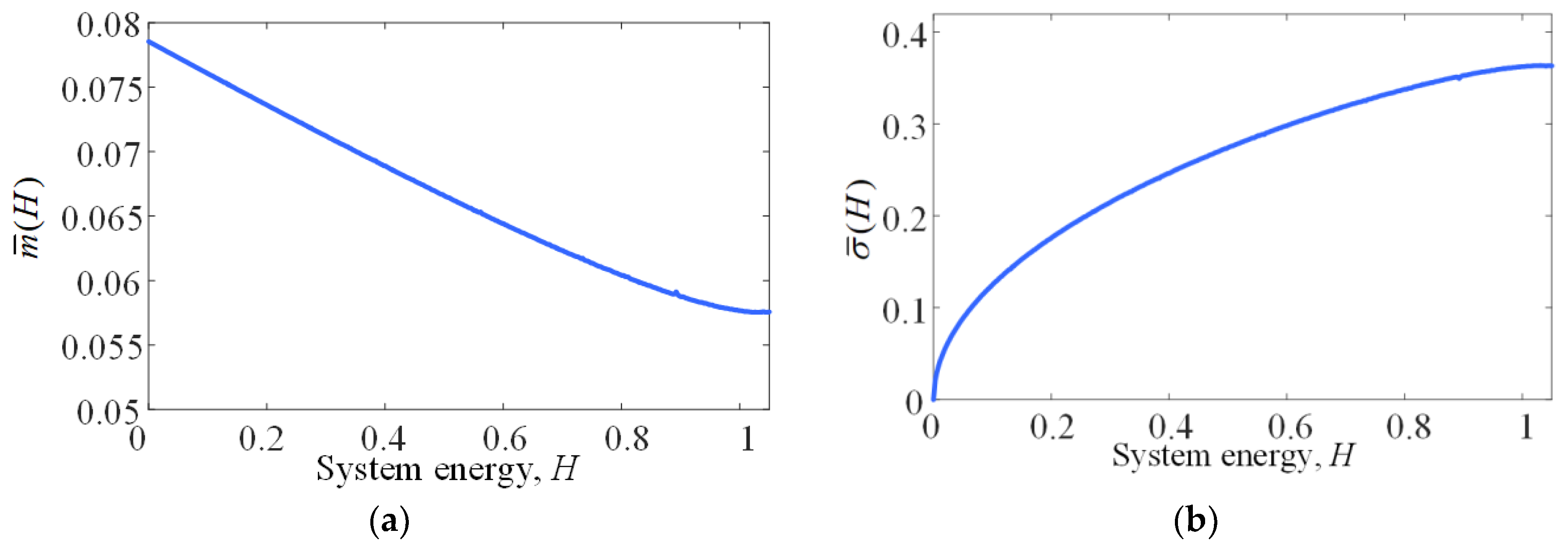
4.2. Equivalent Itō Stochastic Differential Equation for the System Energy of Power Systems with Losses under SCDs

If there are no stochastic disturbances in Equation (5) (i.e., the deterministic model (Equation (2))), the differential function of the system energy can be derivated as follows:

$$\mathrm{d}H=(\partial H/\partial \omega )\mathrm{d}\omega +(\partial H/\partial \delta )\mathrm{d}\delta .$$

(9)

After the introduction of SCDs, the Itō SDEs of the system energy H can be obtained based on the Itō formula [30], which is shown as follows:

$$\begin{array}{ll}\mathrm{d}H& =(\partial H/\partial \omega )\mathrm{d}\omega +(\partial H/\partial \delta )\mathrm{d}\delta +[{\sigma }^2/(2M^2)]({\partial }^{2}H/\partial {\omega }^2)\mathrm{d}t\\ & =[-D{\omega }_{\mathrm{N}}{\omega }^2+{\sigma }^2{\omega }_{\mathrm{N}}/(2M)]\mathrm{d}t+\sigma {\omega }_{\mathrm{N}}\omega \mathrm{d}B(t)\end{array}$$

(10)

where [σ²/(2M²)](∂²H/∂ω²) is the Wong–Zakai correction term [30], B(t) is the Wiener process, and dB(t)/dt = W(t).

Furthermore, by utilizing the stochastic averaging method, the Hamiltonian (i.e., the system energy) weakly converges with a one-dimensional diffusion process, which can be regarded as the equivalent Itō SDEs for Equation (10), as follows:

$$\mathrm{d}H=\overline{m}(H)\mathrm{d}t+\overline{\sigma }(H)\mathrm{d}B(t)$$

(11)

where

$$\{\begin{array}{c}\overline{m}(H)=\frac{1}{T(H)}{\displaystyle {\int }_{\mathsf{\Omega }}\left\{[-D{\omega }_{\mathrm{N}}{\omega }^2+{\sigma }^2{\omega }_{\mathrm{N}}/(2M)]/(\partial H/\partial \omega )\right\}}\mathrm{d}\delta \\ {\overline{\sigma }}^2(H)=\frac{1}{T(H)}{\displaystyle {\int }_{\mathsf{\Omega }}\left[{(\sigma {\omega }_{\mathrm{N}}\omega )}^2/(\partial H/\partial \omega )\right]\times \mathrm{d}\delta }\\ T(H)={\displaystyle {\int }_{\mathsf{\Omega }}\left[1/(\partial H/\partial \omega )\right]\times \mathrm{d}\delta }\\ \mathsf{\Omega }=\left\{\left(\delta \right)|H(\delta ,0)\le H\right\}\end{array}.$$

(12)

4.3. Analytical Method for Solving the Stability Probability

The final step in the proposed assessment method is the application of the Kolmogorov backward equation to solve for the stability probability.

After the stochastic averaging, the system energy of the complex stochastic system (Equation (7)) is equivalent to the diffusion process (Equation (11)). The stability probability (Equation (6) can be regarded as the first-passage probability of the diffusion process (Equation (11)). In probability theory, the Kolmogorov backward equation is often used to characterize stochastic processes. To be specific, the Kolmogorov backward equation describes how the probability that a stochastic process is in a certain region changes over time. Based on the Kolmogorov backward equation, the stability probability is calculated by the following equation:

$$\partial P\left(\begin{array}{ccc}t& |& H_0\end{array}\right)/\partial t=\overline{m}(H_0)\partial P\left(\begin{array}{ccc}t& |& H_0\end{array}\right)/\partial H_0+\frac{1}{2}\overline{\sigma }{(H_0)}^2{\partial }^{2}P\left(\begin{array}{ccc}t& |& H_0\end{array}\right)/\partial H_0{}^2$$

(13)

where H₀ denotes the initial system energy (i.e., the system energy at t = 0).

For the partial differential Equation (13), initial and boundary conditions should be given for the region where solutions of stability probability P(t|H₀) will be solved [31].

Firstly, the initial system energy H₀ should be smaller than the critical system energy H_cr, the stability probability P(t|H₀) at t = 0 is equal to 1, which represents the initial condition. If the initial system energy H₀ exceeds the critical energy H_cr, the stability probability P(t|H₀) should be 0 all the time, which represents a boundary condition. Meanwhile, the stability probability P(t|H₀) with initial energy H₀ should be higher than 0 all the time, which represents another boundary condition. These associated conditions for Equation (13) are shown as follows [25]:

$$\{\begin{array}{l}P(0|H_0)=1, \mathrm{when} H_0<H_{cr}\\ P(t|H_{cr})=0\\ \partial P/\partial t=\overline{m}(0) \partial P/\partial H_0, \mathrm{when} H_0=0\end{array}.$$

(14)

Usually, the partial differential equation based on the Kolmogorov backward equation (Equation (13)) is hard to solve directly. In this paper, the Crank–Nicolson method is adopted to solve Equation (10) to obtain stability probability [31].

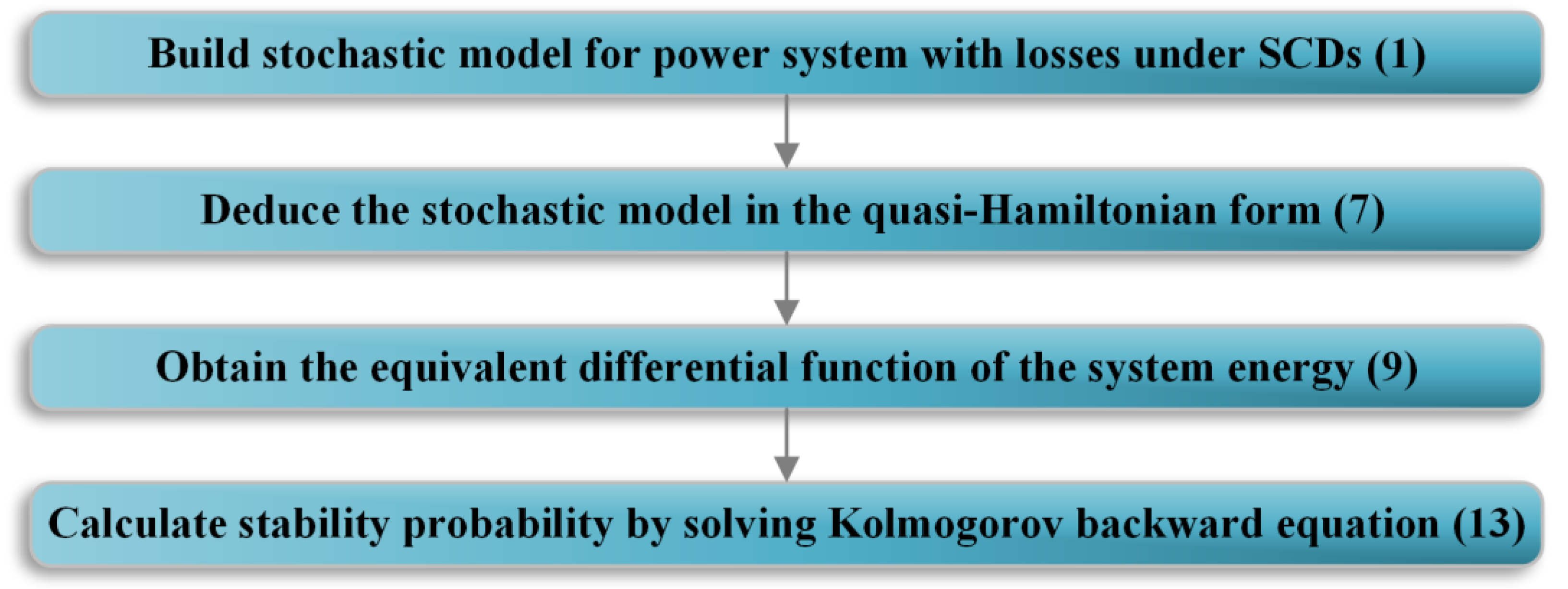
4.4. Procedure for the Stochastic Stability Analysis of a Power System with Losses

The procedure for the stochastic stability analysis of a power system with losses by the stochastic averaging method is outlined below and shown in Figure 1.

Step 1: Build the stochastic model of the power system with losses under SCDs (Equation (1)).

Step 2: Deduce the stochastic model in the quasi-Hamiltonian form (Equation (7)).

Step 3: Obtain the equivalent differential function of the system energy (Equation (9)), based on the stochastic averaging method.

Step 4: Calculate the stability probability of the power system with losses under SCDs, by solving the Kolmogorov backward equation (Equation (13)) based on the Crank–Nicolson method.

5. Simulation Case

5.1. Modified SMIB System and Its Critical Potential Energy

In this section, a modified SMIB system is adopted to verify the proposed method. This system includes losses and SCDs. The model of this system is described by Equation (2), and the corresponding parameters are given as follows: ω_N = 314.16, M = 20, P = 1.1184, E = U = 1, Y₁₂ = 2, α = 6°, D = 05, σ = 0.1, and δ_s = 40°.

Based on the potential energy (Equation (4)), the relation between the potential energy H_P and the rotor angle δ is shown in Figure 2. It can be seen that Point A (δ = δ_s = 34°) is the stable equilibrium point, which represents the stable state of the system; Point B (δ = π − δ_s − 2α = 152°) is the unstable equilibrium point, whose energy is the critical potential energy. Furthermore, the critical potential energy is calculated as H_cr = H_P(152°) = 1.13.

5.2. Stochastic Averaging Method

If system energy exceeds critical potential energy, the system is unstable. When SCDs are introduced into a power system, random events occur, and system energy is lower than critical potential energy, which should be determined by the probability. In this paper, this probability is defined as the stability probability, and the stochastic averaging method is used to analytically calculate it. The stability probability of a power system is equal to the first-passage probability (Equation (13)) of the diffusion process (Equation (11).

After the stochastic averaging method is utilized, the equivalent diffusion process can be obtained. Based on the analysis in Section 4.2, the coefficients (i.e., $\overline{m}$(H) and $\overline{\sigma }$(H)) of the equivalent Itō SDE for the system energy can be calculated, and are illustrated in Figure 3.

Stability probability was calculated based on Equation (13), which is shown here as the red line in Figure 4. To verify the proposed method based on Equation (13), a Monte Carlo simulation was also utilized to calculate the stability probability, which is shown as the black dotted line in Figure 4. As can be seen in Figure 4, the analytical results agree well with those of the Monte Carlo simulation.

This analytical method also has a large advantage in time consumption. Based on the energy function method, the trajectories of the system state should be calculated first, and the system energy can then be calculated based on the trajectories of the system energy. Even though stability is directly assessed by judging whether the system state trajectories are unstable, iterations, which cost most time, are still necessary for Monte Carlo simulations. In Monte Carlo simulations, system state trajectories are simulated by repeated trials based on the stochastic model of power system with losses under SCDs (Equation (1)), which is the major reason that much computation is needed in Monte Carlo simulations.

From these respects, the proposed analytical method is superior, due to its higher efficiency and clearer mechanism. Moreover, since the proposed method is analytical, it can offer accurate results directly without iterations. Hence, the proposed method could work well to analyze the stochastic stability in power systems with losses under SCDs.

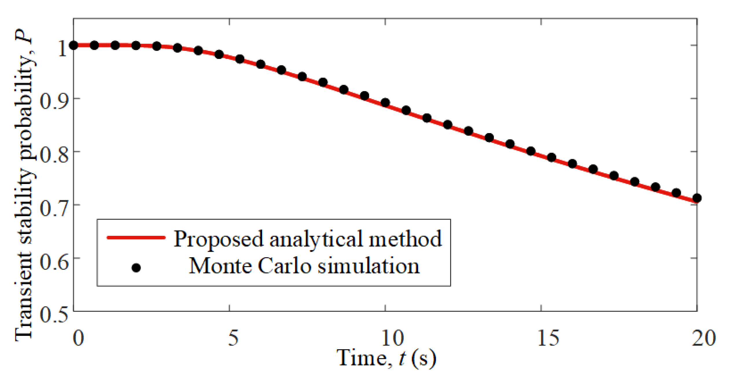
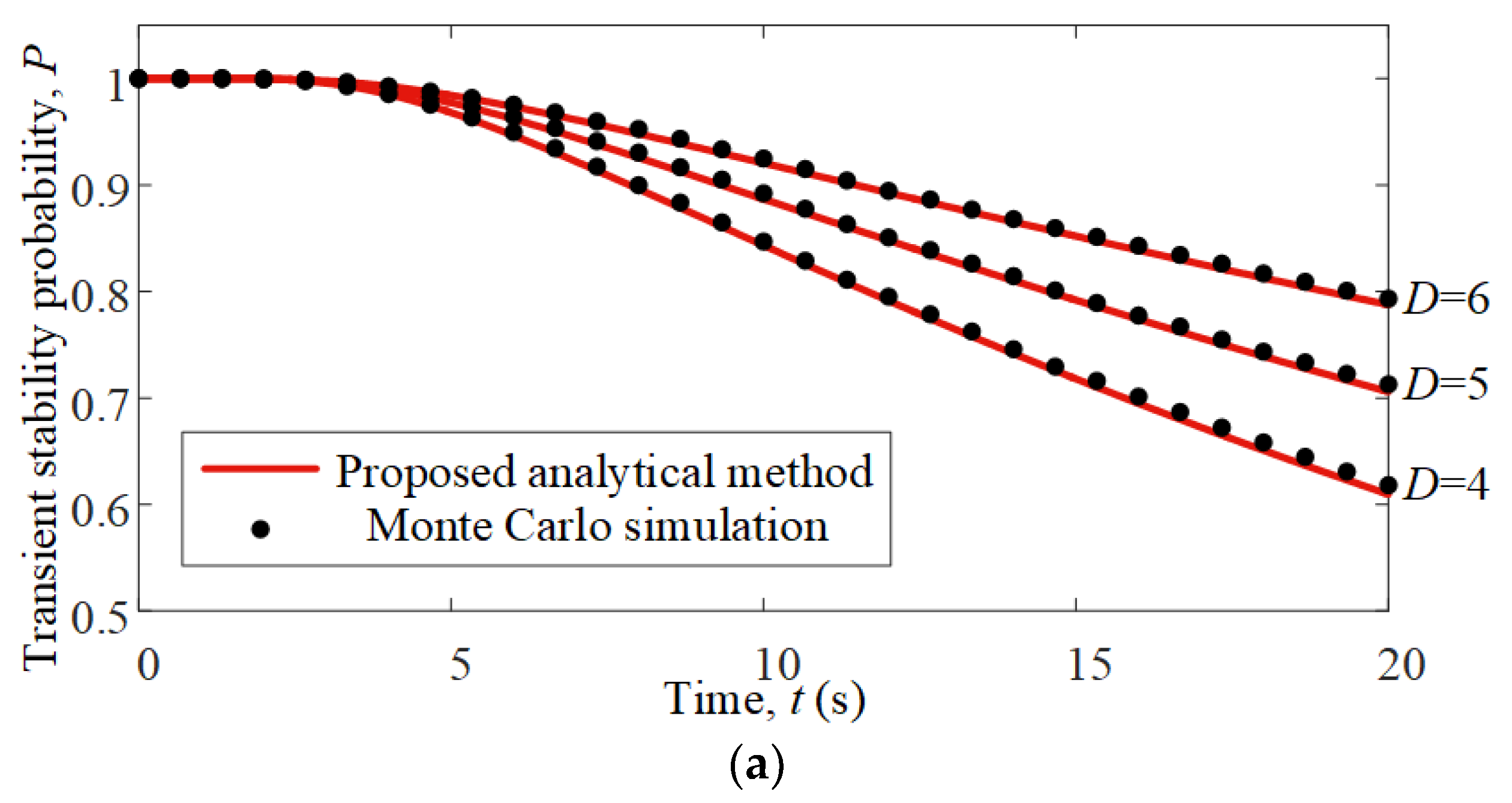
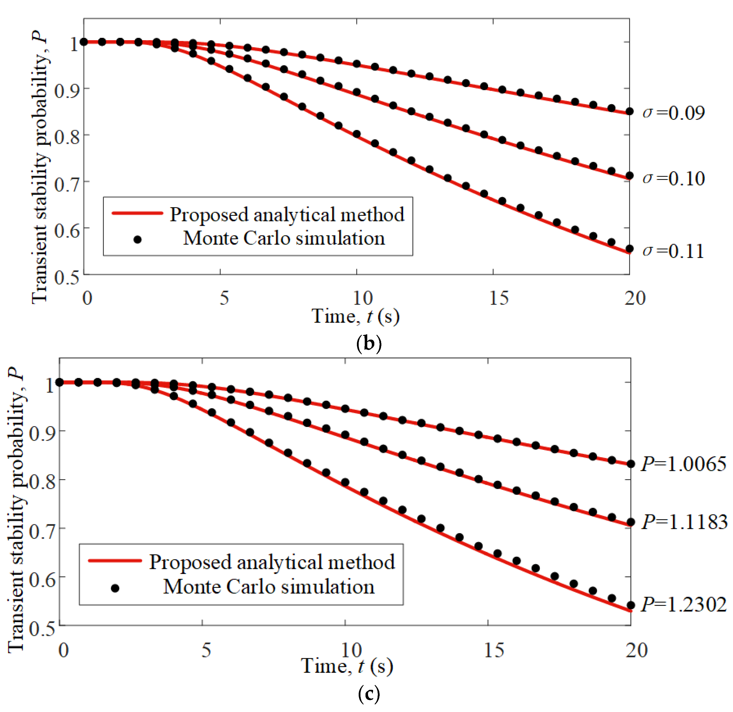
5.3. Comparisons of Stability Probability under Different Parameters

To study the impacts of parameters on the stability probability in power systems with losses under SCDs, several simulation cases, with different damping coefficients, different intensities of SCDs, and different mechanical power levels (which are included in P), were considered, and results are shown in Figure 5. When the mechanical power varies, the system energy function and the critical energy change accordingly. Based on Figure 5, the results of the proposed method agree well with those of the Monte Carlo simulations. Moreover, stability probability decreases as the damping coefficient decreases, as the intensity of SCDs increases, and as the mechanical power increases. These results suggest that the operations on enlarging system damping, mitigating SCDs, and reducing the generation level can improve stability probability.

6. Conclusions

Since intermittent renewable energy and electric vehicles have become involved in power systems, SCDs have attracted much attention. One of the major concerns is whether SCDs influence stability. In this paper, to assess the stability of a power system with losses under SCDs, a stochastic averaging based analytical method is employed. The main contributions of this work are as follows:

(1)

Based on the presented quasi-Hamiltonian model of a power system with losses under SCDs, the quasi-Hamiltonian theory is shown here to be useful in analyzing nonlinear stochastic dynamics in power systems with losses under SCDs.

(2)

The analytical method put forward, which determines the stability probability of a power system with losses under SCDs, agree well with the results of the Monte Carlo simulation. The proposed method is also shown to have a clearer impact mechanism and have higher efficiency.

(3)

The comparisons of stability probability under different parameters are performed, from which insights to improve the stability probability of power systems with losses under SCDs can be obtained.

References

1. Gan, C.; Wu, J.H.; Hu, Y.H.; Yang, S.Y.; Cao, W.P.; Guerrero, J.M. New integrated multilevel converter for switched reluctance motor drives in plug-in hybrid electric vehicles with flexible energy conversion. IEEE Trans. Power Electron. 2017, 32, 3754–3766. [Google Scholar] [CrossRef]
2. Zhou, Y.C.; Li, Y.G.; Liu, W.D.; Yu, D.S.; Li, Z.C.; Liu, J.M. The stochastic response surface method for small-signal stability study of power system with probabilistic uncertainties in correlated photovoltaic and loads. IEEE Trans. Power Syst. 2017, 32, 4551–4559. [Google Scholar] [CrossRef]
3. Zhu, Q.; Chen, J.; Zhu, L.; Duan, X.; Liu, Y. Wind speed prediction with spatio-temporal correlation: A deep learning approach. Energies 2018. to be published. [Google Scholar]
4. Calif, R.; Schmitt, F.G.; Huang, Y.X. Multifractal description of wind power fluctuations using arbitrary order hilbert spectral analysis. Physica A 2013, 392, 4106–4120. [Google Scholar] [CrossRef]
5. Zhou, T.P.; Sun, W. Optimization of battery-supercapacitor hybrid energy storage station in wind/solar generation system. IEEE Trans. Sustain. Energy 2014, 5, 408–415. [Google Scholar] [CrossRef]
6. Jia, H.J.; Mu, Y.F.; Qi, Y. A statistical model to determine the capacity of battery-supercapacitor hybrid energy storage system in autonomous microgrid. Int. J. Electr. Power Energy Syst. 2014, 54, 516–524. [Google Scholar] [CrossRef]
7. Perez-Ortiz, M.; Jimenez-Fernandez, S.; Gutierrez, P.; Alexandre, E.; Hervas-Martinez, C.; Salcedo-Sanz, S. A review of classification problems and algorithms in renewable energy applications. Energies 2016, 9, 607. [Google Scholar] [CrossRef]
8. Ehsani, M.; Falahi, M.; Lotfifard, S. Vehicle to grid services: Potential and applications. Energies 2012, 5, 4076–4090. [Google Scholar] [CrossRef]
9. Wang, T.; Bi, T.; Wang, H.; Liu, J. Decision tree based online stability assessment scheme for power systems with renewable generations. CSEE J. Power Energy Syst. 2015, 1, 53–61. [Google Scholar] [CrossRef]
10. Zhang, J.Y.; Ju, P.; Yu, Y.P.; Wu, F. Responses and stability of power system under small gauss type random excitation. Sci. China-Technol. Sci. 2012, 55, 1873–1880. [Google Scholar] [CrossRef]
11. Qiu, J.; Shahidehpour, S.M.; Schuss, Z. Effect of small random perturbations on power-systems dynamics and its reliability evaluation. IEEE Trans. Power Syst. 1989, 4, 197–204. [Google Scholar] [CrossRef]
12. Ma, J.; Song, Z.X.; Zhang, Y.X.; Zhao, Y.; Thorp, J.S. Robust stochastic stability analysis method of dfig integration on power system considering virtual inertia control. IEEE Trans. Power Syst. 2017, 32, 4069–4079. [Google Scholar] [CrossRef]
13. Odun-Ayo, T.; Crow, M.L. Structure-preserved power system transient stability using stochastic energy functions. IEEE Trans. Power Syst. 2012, 27, 1450–1458. [Google Scholar] [CrossRef]
14. Wang, K.; Crow, M.L. The fokker-planck equation for power system stability probability density function evolution. IEEE Trans. Power Syst. 2013, 28, 2994–3001. [Google Scholar] [CrossRef]
15. Hua, K.; Mishra, Y.; Ledwich, G. Fast unscented transformation-based transient stability margin estimation incorporating uncertainty of wind generation. IEEE Trans. Sustain. Energy 2015, 6, 1254–1262. [Google Scholar] [CrossRef]
16. Zarate-Minano, R.; Anghel, M.; Milano, F. Continuous wind speed models based on stochastic differential equations. Appl. Energy 2013, 104, 42–49. [Google Scholar] [CrossRef]
17. Ghanavati, G.; Hines, P.D.H.; Lakoba, T.I. Identifying useful statistical indicators of proximity to instability in stochastic power systems. IEEE Trans. Power Syst. 2016, 31, 1360–1368. [Google Scholar] [CrossRef]
18. Milano, F.; Zárate-Miñano, R. A systematic method to model power systems as stochastic differential algebraic equations. IEEE Trans. Power Syst. 2013, 28, 4537–4544. [Google Scholar] [CrossRef]
19. Yuan, B.; Zhou, M.; Li, G.; Zhang, X.P. Stochastic small-signal stability of power systems with wind power generation. IEEE Trans. Power Syst. 2015, 30, 1680–1689. [Google Scholar] [CrossRef]
20. Wang, X.; Chiang, H.D.; Wang, J.; Liu, H.; Wang, T. Long-term stability analysis of power systems with wind power based on stochastic differential equations: Model development and foundations. IEEE Trans. Sustain. Energy 2015, 6, 1534–1542. [Google Scholar] [CrossRef]
21. Ju, P.; Li, H.; Pan, X.; Gan, C.; Liu, Y.; Liu, Y. Stochastic dynamic analysis for power systems under uncertain variability. IEEE Trans. Power Syst. 2017, PP, 1. [Google Scholar] [CrossRef]
22. Dong, Z.Y.; Zhao, J.H.; Hill, D.J. Numerical simulation for stochastic transient stability assessment. IEEE Trans. Power Syst. 2012, 27, 1741–1749. [Google Scholar] [CrossRef]
23. Chen, L.C.; Zhu, W.Q. First passage failure of dynamical power systems under random perturbations. Sci. China-Technol. Sci. 2010, 53, 2495–2500. [Google Scholar] [CrossRef]
24. Chen, L.C.; Zhu, W.Q. First passage failure of quasi non-integrable generalized hamiltonian systems. Arch. Appl. Mech. 2010, 80, 883–893. [Google Scholar] [CrossRef]
25. Ju, P.; Li, H.; Gan, C.; Liu, Y.; Yu, Y.; Liu, Y. Analytical assessment for transient stability under stochastic continuous disturbances. IEEE Trans. Power Syst. 2018, 33, 2004–2014. [Google Scholar] [CrossRef]
26. Zhu, W.Q. Nonlinear stochastic dynamics and control in hamiltonian formulation. Appl. Mech. Rev. 2006, 59, 230–248. [Google Scholar] [CrossRef]
27. Zhu, W.Q.; Yang, Y.Q. Stochastic averaging of quasi-nonintegrable-hamiltonian systems. J. Appl. Mech.-Trans. Asme 1997, 64, 157–164. [Google Scholar] [CrossRef]
28. Hsiao-Dong, C.; Chia-Chi, C.; Cauley, G. Direct stability analysis of electric power systems using energy functions: Theory, applications, and perspective. Proc. IEEE 1995, 83, 1497–1529. [Google Scholar] [CrossRef]
29. Ortega, R.; Galaz, M.; Astolfi, A.; Yuanzhang, S.; Shen, T. Transient stabilization of multimachine power systems with nontrivial transfer conductances. IEEE Trans. Autom. Control 2005, 50, 60–75. [Google Scholar] [Green Version]
30. Mao, X. Stochastic Differential Equations and Applications; Elsevier: Amsterdam, The Netherlands, 2007. [Google Scholar]
31. Gan, C.; Zhu, W. First-passage failure of quasi-non-integrable-hamiltonian systems. Int. J. Non-Linear Mech. 2001, 36, 209–220. [Google Scholar] [CrossRef]
Figure 1. The procedure of the proposed stochastic stability analysis method. SCD: stochastic disturbance.
Energies 11 00678 g001
Figure 2. Potential energy curve near the stable point.
Energies 11 00678 g002
Figure 3. The coefficients of the equivalent Itō stochastic differential equation for the system energy: (a) the drift coefficient m ¯ (H); (b) the diffusion coefficient σ ¯ (H).
Energies 11 00678 g003
Figure 4. Stability probability of power system with losses under stochastic continuous disturbances.
Energies 11 00678 g004
Figure 5. Stability probability of power system with losses under stochastic continuous disturbances: (a) damping coefficient; (b) intensity of stochastic continuous disturbances; (c) mechanical power.
Energies 11 00678 g005aEnergies 11 00678 g005b