On the Classification of Low Voltage Feeders for Network Planning and Hosting Capacity Studies

Abstract
1. Introduction
- average distance between nodes
- average impedance at the point of connection
- total cable length
- feeder length
- cable or line rating
2. Method and Data Set
2.1. Available Data Set
- descriptive indicators or explanatory variables
- hosting capacity related indicators.
2.2. Presentation of the Concept Used for the Feeder Clustering and Classification
- Clustering consists in grouping a set of observations into clusters, on the unique basis of some observed variables, and without knowing a priori the number of clusters. Observations within a cluster should have at the same time a high similarity between each other and a high dissimilarity with observations in other clusters.
- Classification consists in finding a way to identify to which sub-set of observations (category or class) a new observation belongs. This is done on the basis of an algorithm trained on a set of data containing observations whose category or class is known.
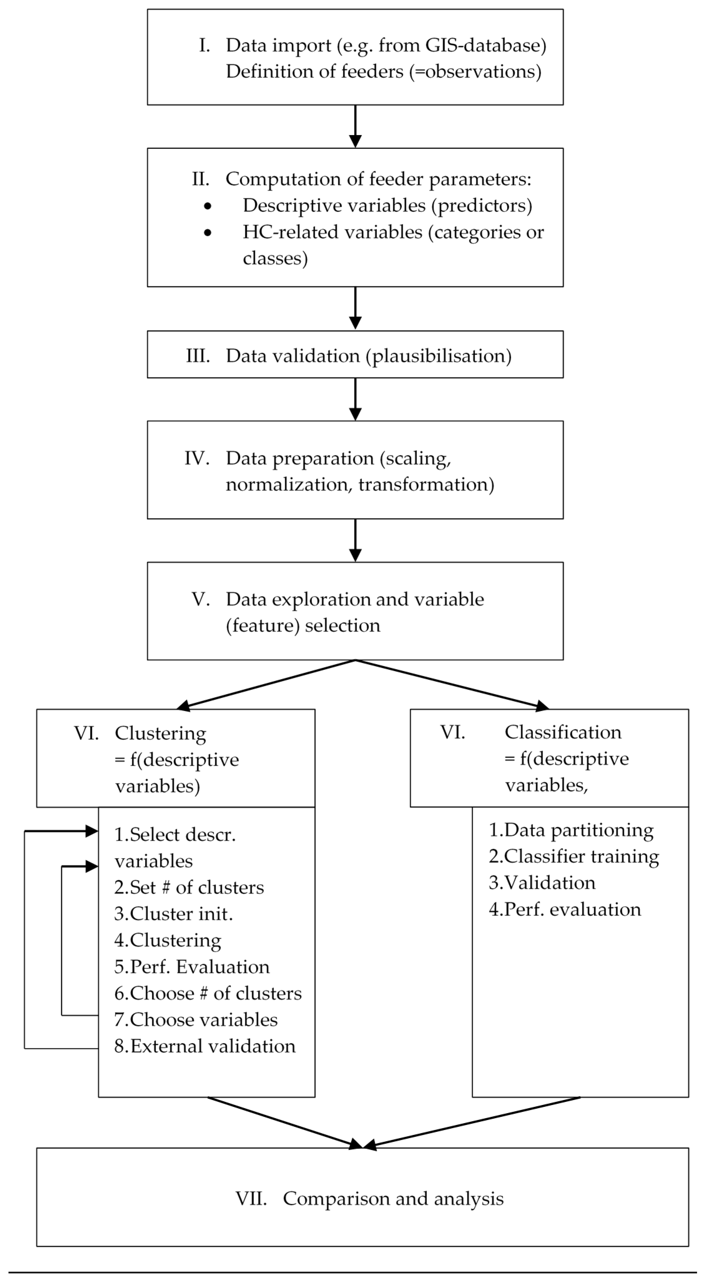
2.2.1. General Concept
- Descriptive variables (predictors)
- Hosting capacity-related variables (categories or classes)
2.2.2. Feeder Clustering (Non-Supervised Learning)
- Feature selection or extraction
- Clustering algorithm design or selection
- Cluster validation
- Result interpretation
2.2.3. Feeder Classification (Supervised Learning)
3. Results
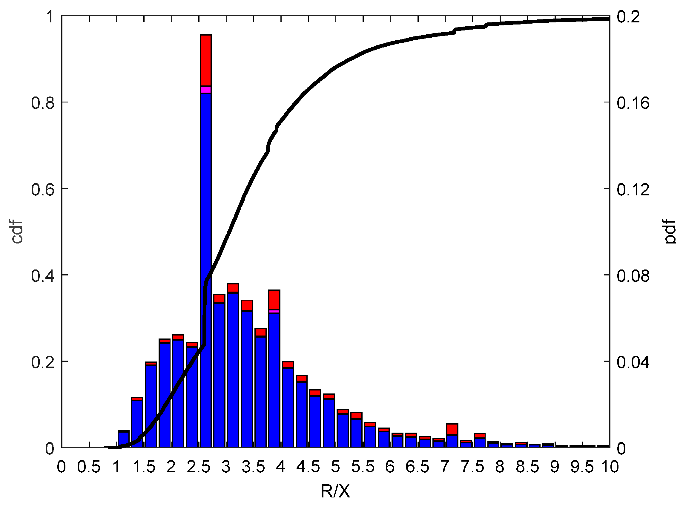
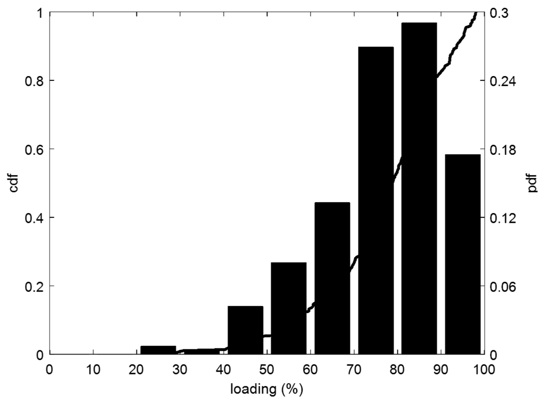
3.1. Statistical Analysis of the Feeders
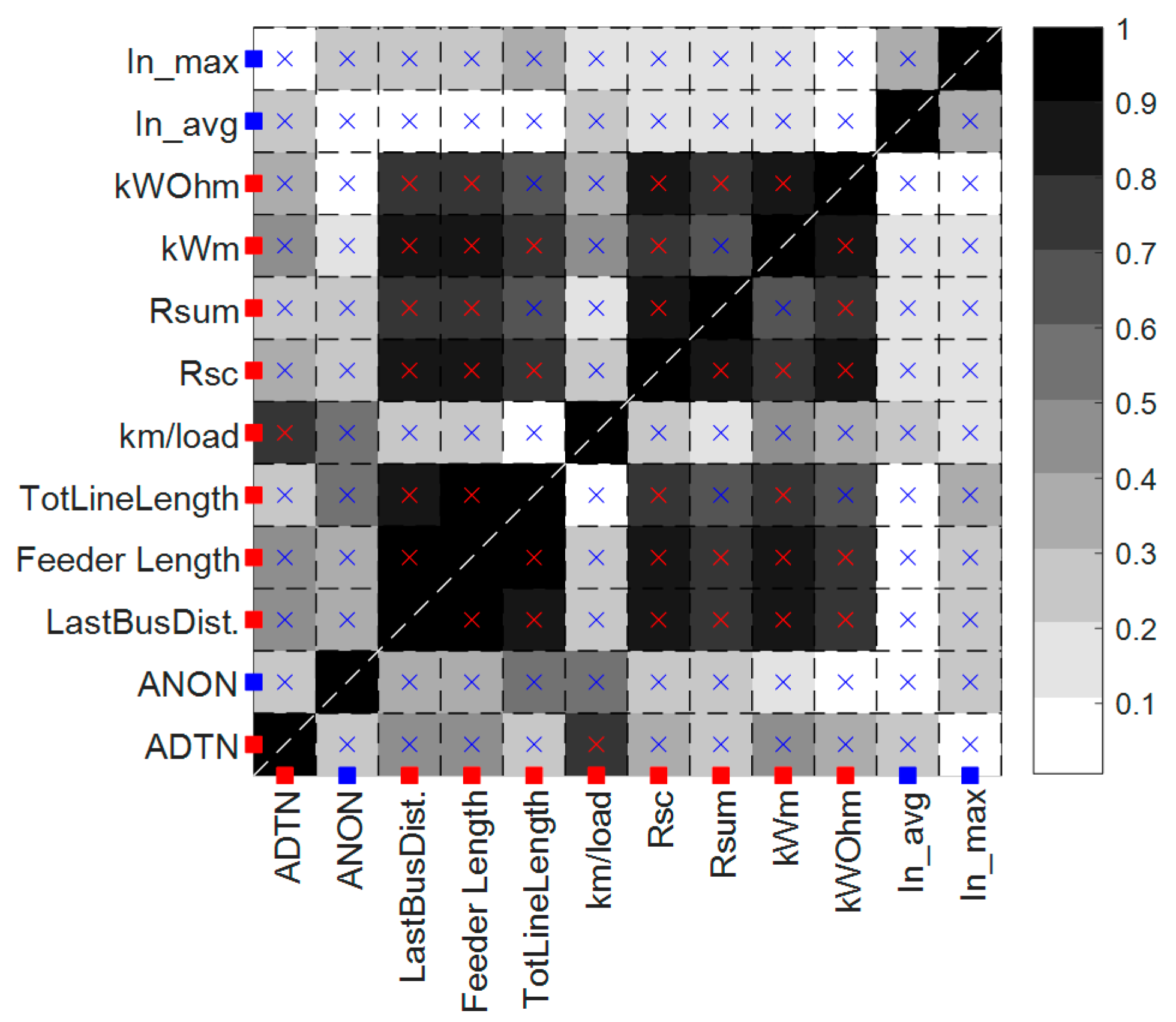
3.2. Parameter Selection and Data Reduction
- Correlation analysis
- Variable clustering (details not shown here)
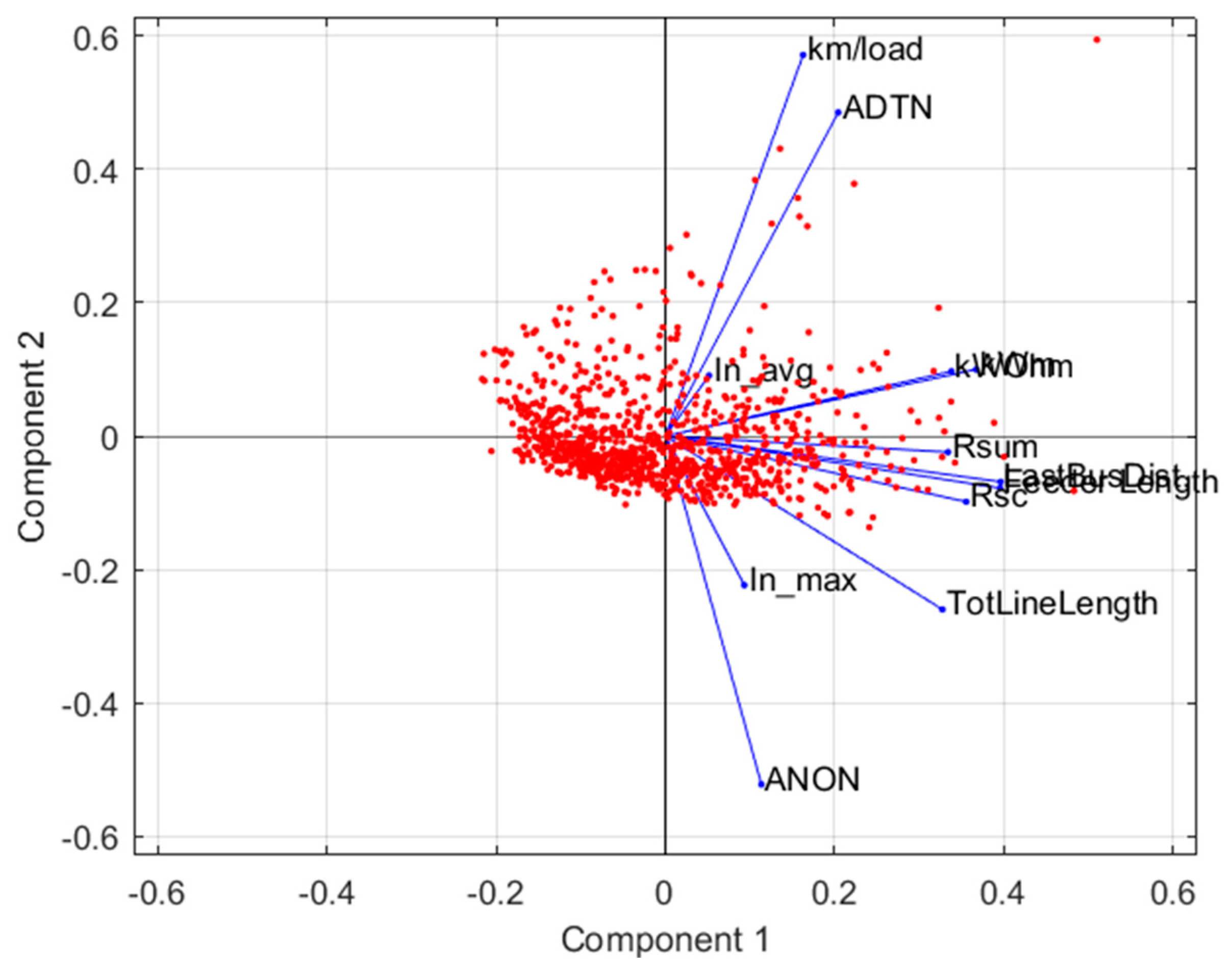
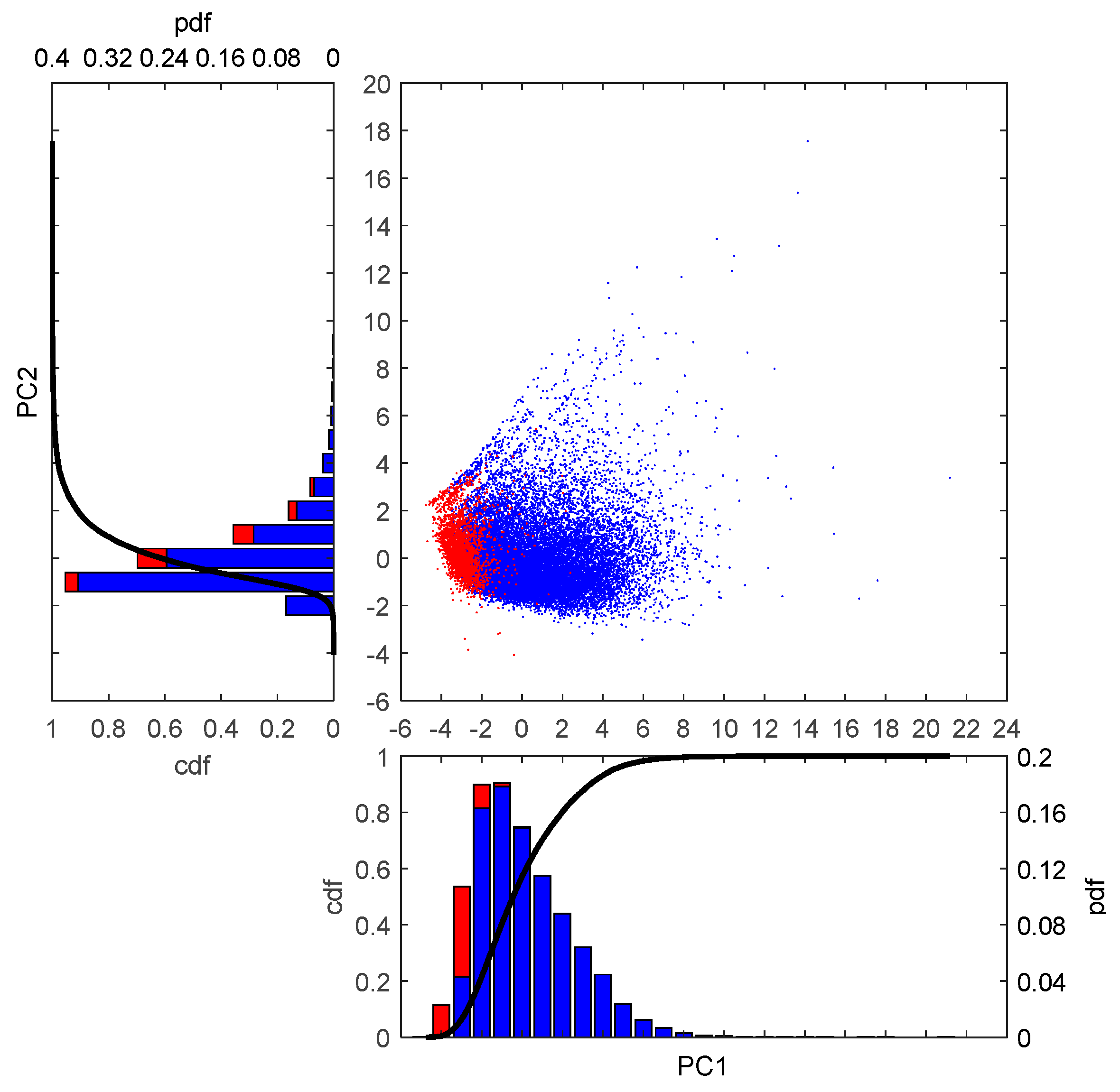
- Principal Component Analysis (PCA)
- In_max
- In_avg
- km/load
- ANON
- Rsum
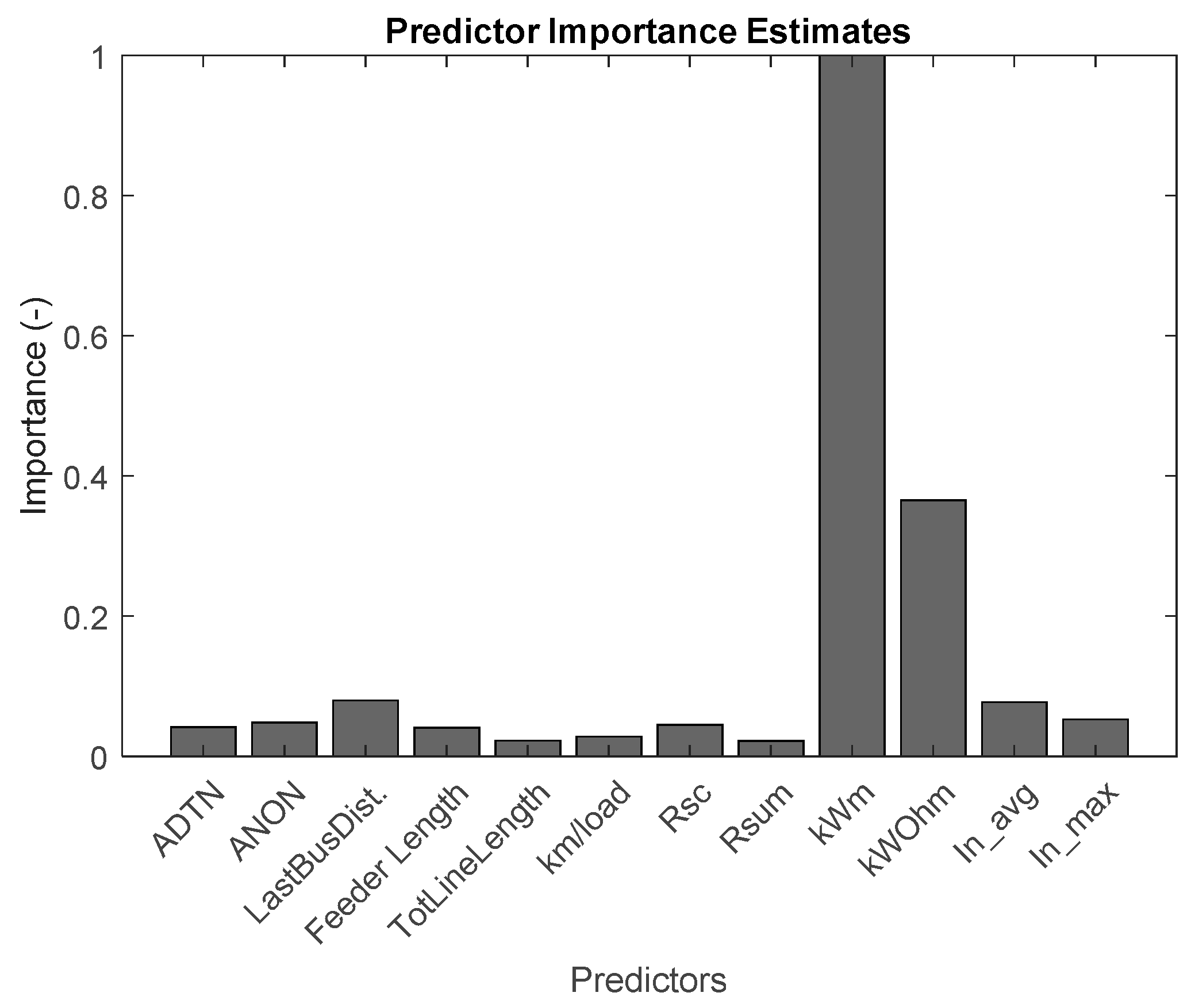
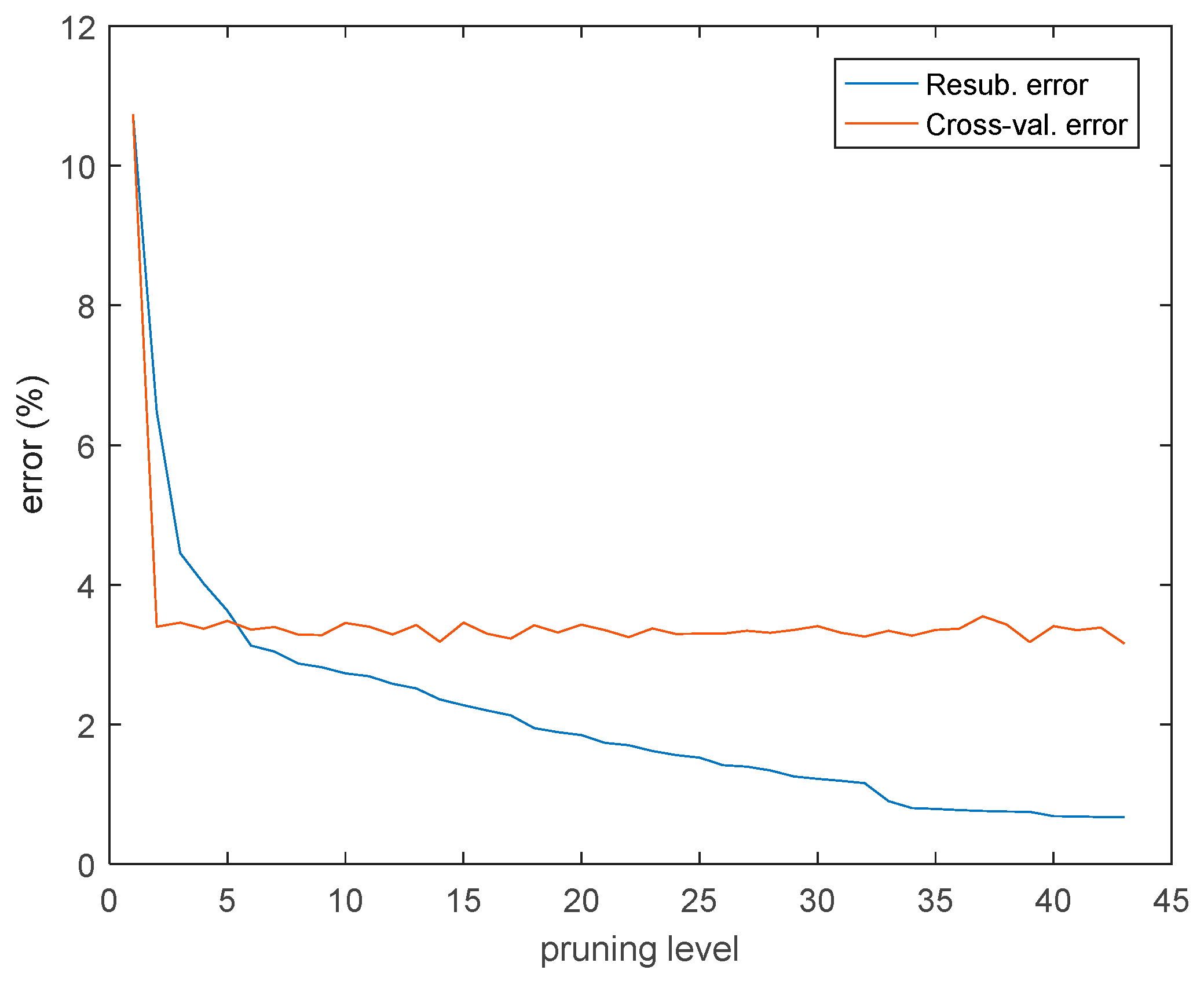
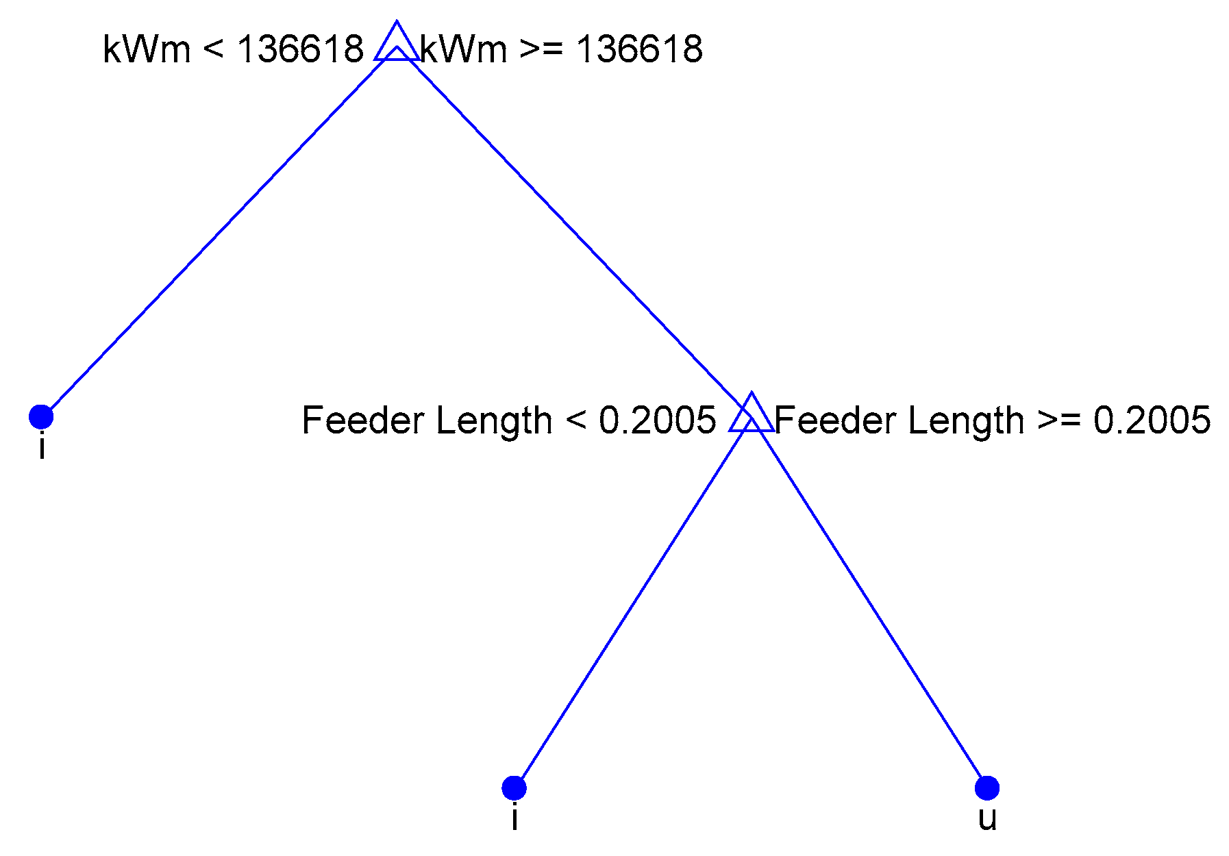
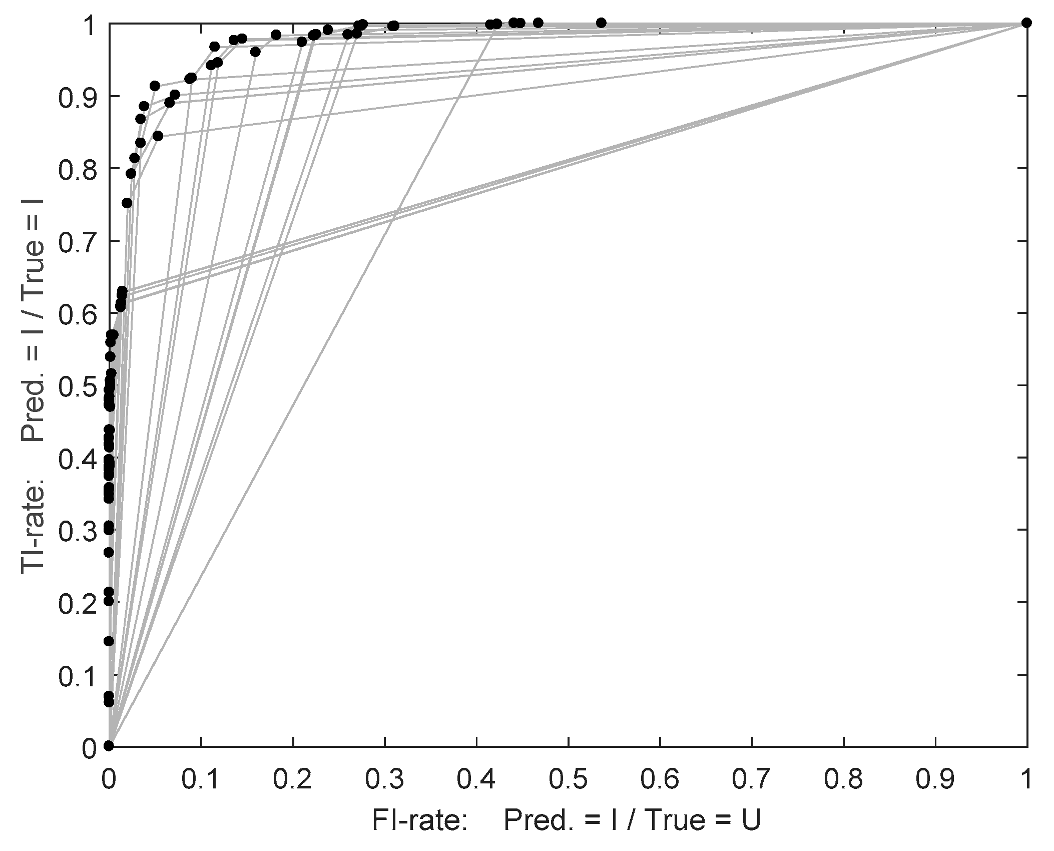
3.3. Classification of LV Feeders
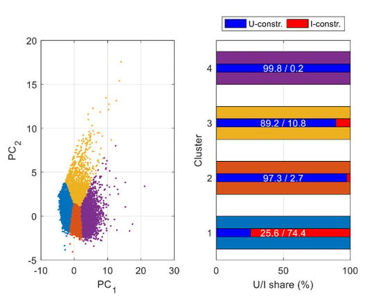
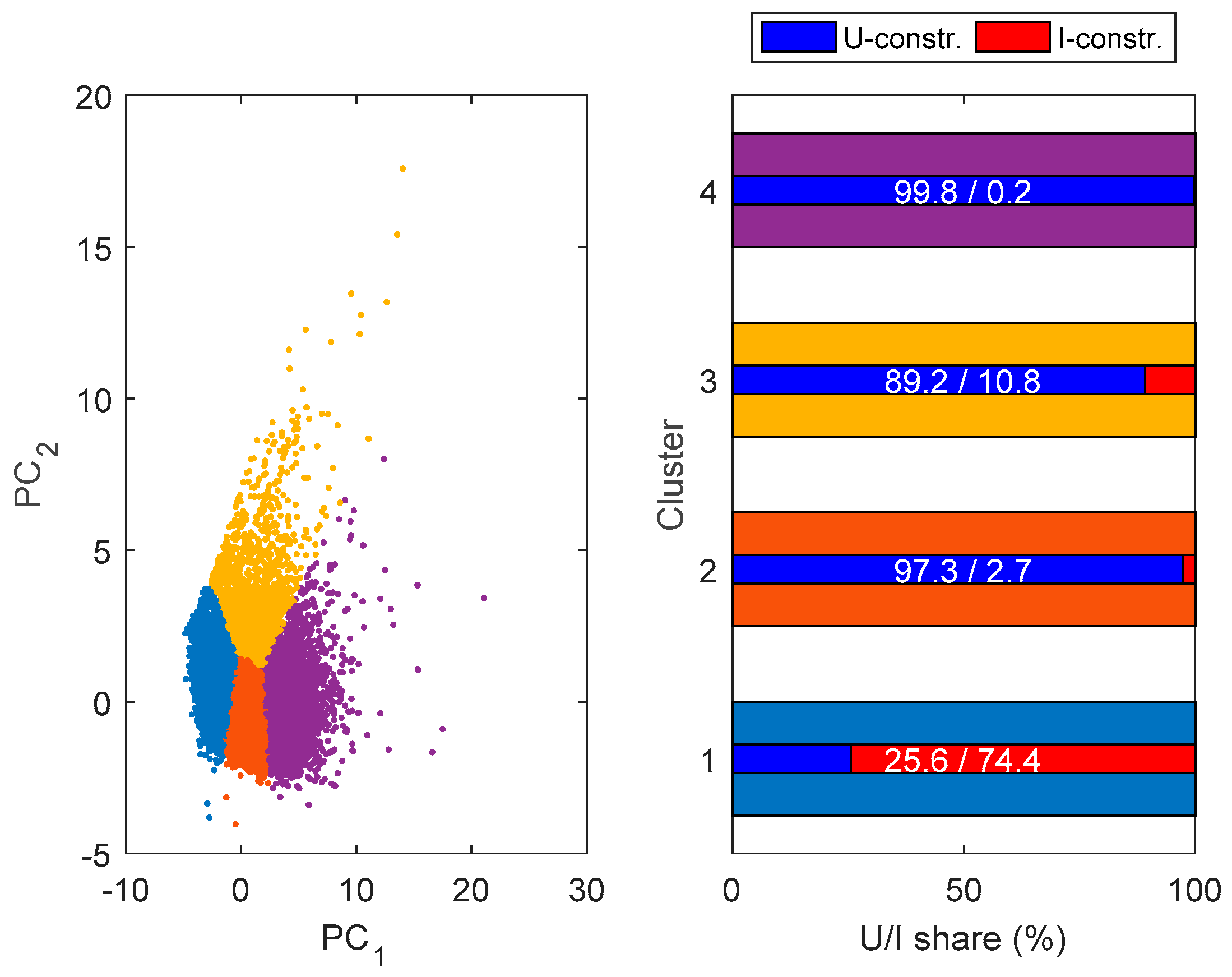
- voltage-constrained feeders
- current-constrained feeders
- Accuracy: probability of a correct classification among the data set (Equation (7))
- Sensitivity: the ability to classify correctly I-constrained feeders among the I-constrained feeders (Equation (8))
- Specificity: the ability to classify correctly U-constrained feeders among the U-constrained feeders (Equation (9))
- False positive rate (false alarm rate): the rate of U-constrained feeders which have been classified as I-constrained feeders (Equation (10)):
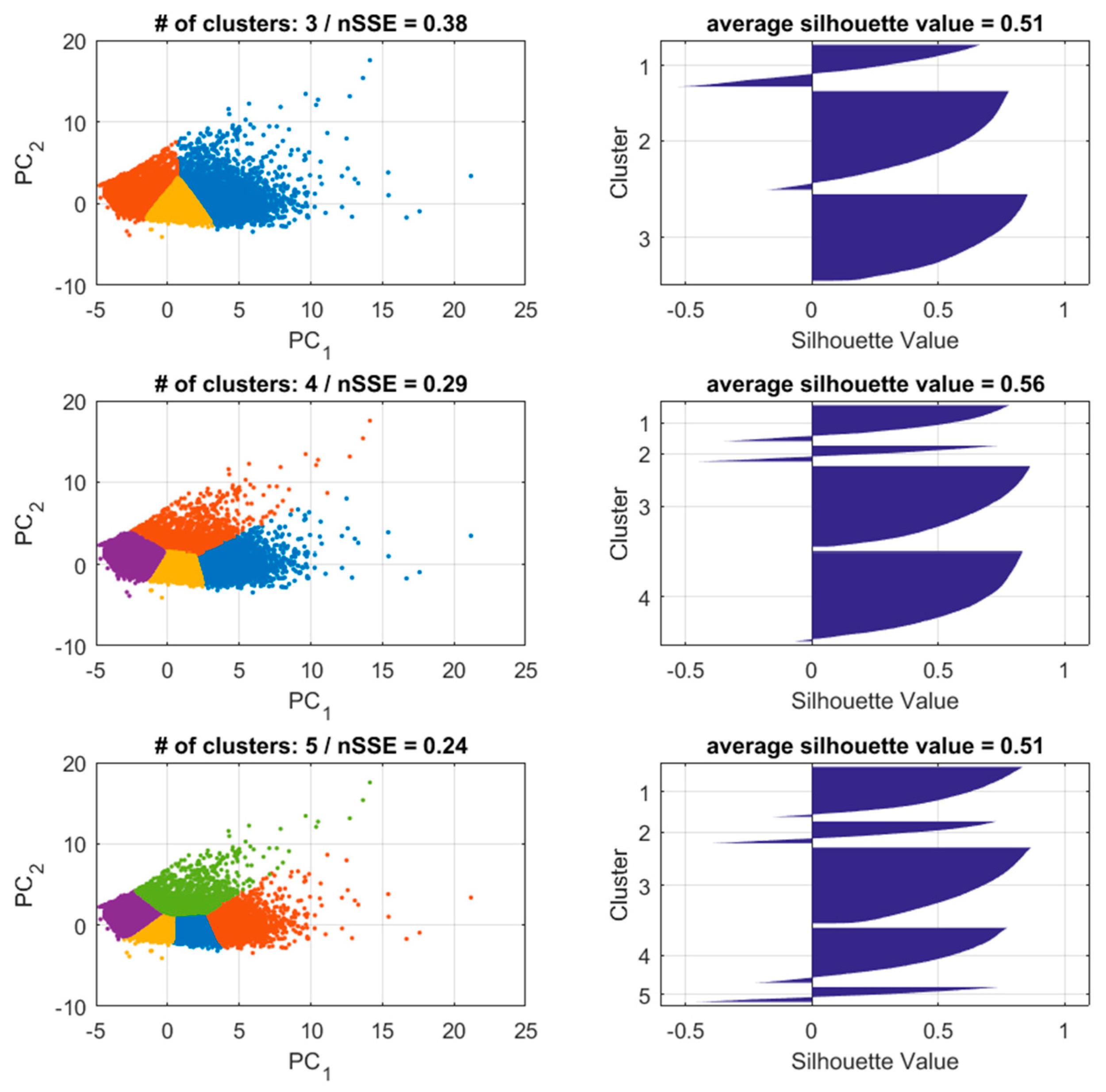
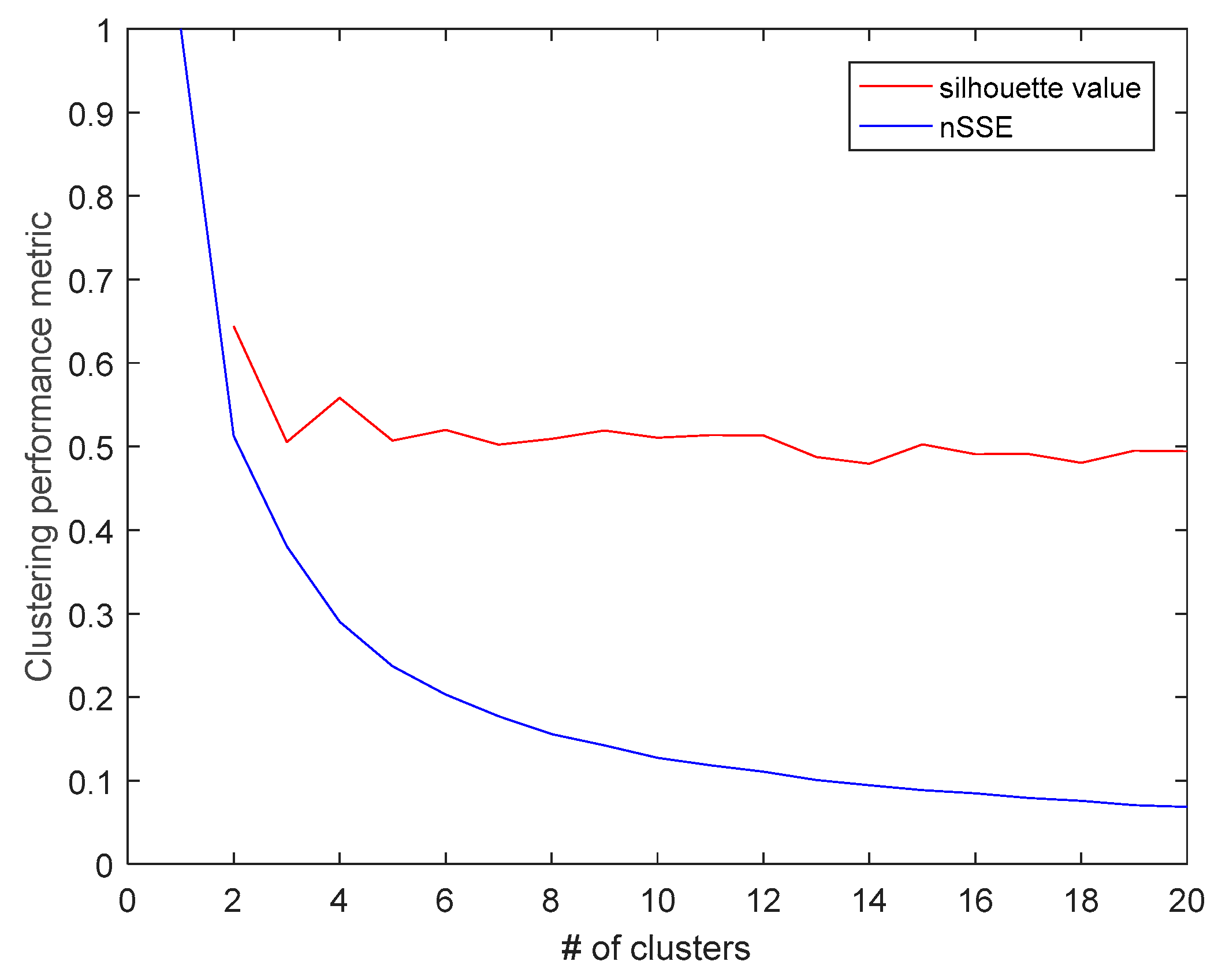
3.4. Clustering of LV Feeders
- Variables used
- Number of clusters used
4. Discussion and Conclusions
Acknowledgments
Author Contributions
Conflicts of Interest
References
- Bollen, M.; Rönnberg, S. Hosting Capacity of the Power Grid for Renewable Electricity Production and New Large Consumption Equipment. Energies 2017, 10, 1325. [Google Scholar]
- Bletterie, B.; Goršek, A.; Uljanić, B.; Jahn, J. Enhancement of the network hosting capacity—Clearing space for/with PV. In Proceedings of the 25th European Photovoltaic Solar Energy Conference and Exhibition, Valencia, Spain, 6–10 September 2010; pp. 4828–4834. [Google Scholar]
- VDE. VDE-AR-N 4105 Generators Connected to the Low-Voltage Distribution Network—Technical Requirements for the Connection to and Parallel Operation with Low-Voltage Distribution Networks; VDE: Frankfurt am Main, Germany, 2017. [Google Scholar]
- Ministère de L’écologie, de L’énergie, du Développement Durable et de L’aménagement du Territoire. Arrêté du 23 Avril 2008 Relatif aux Prescriptions Techniques de Conception et de Fonctionnement Pour le Raccordement à un Réseau Public de Distribution D’électricité en Basse Tension ou en Moyenne Tension D’une installation de Production D’énergie Électrique; Ministère de L’écologie, de L’énergie, du Développement Durable et de L’aménagement du Territoire: Paris, France, 2008.
- E-Control. Technische und Organisatorische Regeln für Betreiber und Benutzer von Netzen. Teil D: Besondere Technische Regeln. Hauptabschnitt D4: Parallelbetrieb von Erzeugungsanlagen mit Verteilernetzen; E-Control: Vienna, Austria, 2016. [Google Scholar]
- Bletterie, B.; Gorsek, A.; Fawzy, T.; Premm, D.; Deprez, W.; Truyens, F.; Woyte, A.; Blazic, B.; Uljanic, B. Development of innovative voltage control for distribution networks with high photovoltaic penetration: Voltage control in high PV penetration networks. Prog. Photovolt. Res. Appl. 2012, 20, 747–759. [Google Scholar] [CrossRef]
- Kadam, S.; Bletterie, B.; Lauss, G.; Heidl, M.; Winter, C.; Hanek, D.; Abart, A. Evaluation of voltage control algorithms in smart grids: Results of the project: MorePV2grid. In Proceedings of the 29th European Photovoltaic Solar Energy Conference and Exhibition, Amsterdam, The Netherlands, 22–26 September 2014. [Google Scholar]
- Stetz, T.; Marten, F.; Braun, M. Improved Low Voltage Grid-Integration of Photovoltaic Systems in Germany. IEEE Trans. Sustain. Energy 2013, 4, 534–542. [Google Scholar] [CrossRef]
- Dehghani, F.; Nezami, H.; Dehghani, M.; Saremi, M. Distribution feeder classification based on self organized maps (case study: Lorestan province, Iran). In Proceedings of the 20th Conference on Electrical Power Distribution Networks Conference (EPDC), Zahedan, Iran, 28–29 April 2015; pp. 27–31. [Google Scholar]
- Nijhuis, M.; Gibescu, M.; Cobben, S. Clustering of low voltage feeders from a network planning perspective. In Proceedings of the CIRED 23rd International Conference on Electricity Distribution, Lyon, France, 15–18 June 2015. [Google Scholar]
- Willis, H.L.; Tram, H.N.; Powell, R.W. A Computerized, cluster based method of building representative models of distribution systems. IEEE Trans. Power Appar. Syst. 1985, 12, 3469–3474. [Google Scholar] [CrossRef]
- Schneider, K.P.; Chen, Y.; Chassin, D.P.; Pratt, R.G.; Engel, D.W.; Thompson, S. Modern Grid Initiative: Distribution Taxonomy Final Report; Pacific Northwest National Laboratory: Richland, WA, USA, 2008. [Google Scholar]
- Kerber, G. Aufnahmefähigkeit von Niederspannungsverteilnetzen für die Einspeisung aus Photovoltaikkleinanlagen; Technical University of Munich: Munich, Germany, 2011. [Google Scholar]
- Lindner, M.; Aigner, C.; Witzmann, R.; Frings, R. Aktuelle Musternetze zur Untersuchung von Spannungsproblemen in der Niederspannung. In Proceedings of the 14 Symposium Energieinnovation, Graz, Austria, 10–12 February 2016. [Google Scholar]
- DeNA. DeNA-Verteilernetzstudie. Ausbau-und Innovationsbedarf der Stromverteilnetze in Deutschland bis 2030; DeNA: Tokyo, Japan, 2012. [Google Scholar]
- Dickert, J.; Domagk, M.; Schegner, P. Benchmark low voltage distribution networks based on cluster analysis of actual grid properties. In Proceedings of the 2013 IEEE Grenoble Conference on PowerTech (POWERTECH), Grenoble, France, 16–20 June 2013; pp. 1–6. [Google Scholar]
- Broderick, R.J.; Williams, J.R. Clustering methodology for classifying distribution feeders. In Proceedings of the 2013 IEEE 39th Photovoltaic Specialists Conference (PVSC), Tampa, FL, USA, 16–21 June 2013; pp. 1706–1710. [Google Scholar]
- Gust, G. Analyse von Niederspannungsnetzen und Entwicklung von Referenznetzen; KIT: Cornwall, UK, 2014. [Google Scholar]
- Cale, J.; Palmintier, B.; Narang, D.; Carroll, K. Clustering distribution feeders in the Arizona Public Service territory. In Proceedings of the 2014 IEEE 40th Photovoltaic Specialist Conference (PVSC), Denver, Colorado, 8–13 June 2014; pp. 2076–2081. [Google Scholar]
- Li, Y.; Wolfs, P.J. Taxonomic description for western Australian distribution medium-voltage and low-voltage feeders. IET Gener. Transm. Distrib. 2014, 8, 104–113. [Google Scholar] [CrossRef]
- Walker, G.; Nägele, H.; Kniehl, F.; Probst, A.; Brunner, M.; Tenbohlen, S. An application of cluster reference grids for an optimized grid simulation. In Proceedings of the CIRED 23rd International Conference on Electricity Distribution, Lyon, France, 15–18 June 2015. [Google Scholar]
- Varela, J.; Hatziargyriou, N.; Puglisi, L.J.; Rossi, M.; Abart, A.; Bletterie, B. The IGREENGrid Project: Increasing Hosting Capacity in Distribution Grids. IEEE Power Energy Mag. 2017, 15, 30–40. [Google Scholar] [CrossRef]
- Bletterie, B.; Kadam, S.; Abart, A.; Priewasser, R. Statistical analysis of the deployment potential of Smart Grids solutions to enhance the hosting capacity of LV networks. In Proceedings of the 14 Symposium Energieinnovation, Graz, Austria, 10–12 February 2016. [Google Scholar]
- PowerFactory—DIgSILENT Germany. 2017. Available online: http://www.digsilent.de/index.php/products-powerfactory.html (accessed on 6 November 2015).
- Python. 2017. Available online: https://www.python.org/ (accessed on 21 March 2016).
- Kadam, S.; Bletterie, B.; Gawlik, W. A Large Scale Grid Data Analysis Platform for DSOs. Energies 2017, 10, 1099. [Google Scholar] [CrossRef]
- Bletterie, B.; Abart, A.; Kadam, S.; Burnier, D.; Stifter, M.; Brunner, H. Characterising LV networks on the basis of smart meter data and accurate network models. In Proceedings of the Integration of Renewables into the Distribution Grid (CIRED 2012 Workshop), Lisbon, Portugal, 29–30 May 2012; pp. 1–4. [Google Scholar]
- Xu, R.; Wunsch, D. Survey of Clustering Algorithms. IEEE Trans. Neural Netw. 2005, 16, 645–678. [Google Scholar] [CrossRef] [PubMed]
- Bletterie, B.; Gorsek, A.; Abart, A.; Heidl, M. Understanding the effects of unsymmetrical infeed on the voltage rise for the design of suitable voltage control algorithms with PV inverters. In Proceedings of the 26th European Photovoltaic Solar Energy Conference and Exhibition, Hamburg, Germany, 5–9 September 2011; pp. 4469–4478. [Google Scholar]
- Jenkins, N.; Allan, R.; Crossley, P.; Kirschen, D.; Strbac, G. Embedded Generation; The Institution of Engineering and Technology: London, UK, 2000. [Google Scholar]
- Sutton, C.D. Classification and Regression Trees, Bagging, and Boosting. In Handbook of Statistics; Elsevier: Amsterdam, The Netherlands, 2005; Volume 24, pp. 303–329. [Google Scholar]
- Bradley, A.P. The use of the area under the ROC curve in the evaluation of machine learning algorithms. Pattern Recognit. 1997, 30, 1145–1159. [Google Scholar] [CrossRef]
- Walker, G.; Krauss, A.-K.; Eilenberger, S.; Schweinfort, W.; Tenbohlen, S. Entwicklung eines standardisierten Ansatzes zur Klassifizierung von Verteilnetzen. In VDE-Kongress 2014; VDE Verlag: Berlin, Germany, 2014. [Google Scholar]


| Study | Scope | Target | Data Set | Statistical Method 1 | # of Param. | # of Clusters |
|---|---|---|---|---|---|---|
| Willis et al., 1985 [11] (US) | MV feeders | “representative feeders” | 1350 | k-means | 11 | 10 |
| Schneider et al., 2008 [12] (US) | MV feeders | “prototypal feeders” | 575 | hierarchical | 35 | 24 |
| Nijhuis et al., 2015 [10] (NL) | LV feeders | “most common types of feeders” | 88,000 | fuzzy k-medians | 945→8 2 | 8 |
| Kerber, 2011 [13]/ Lindner et al., 2016 [14] (DE) | LV networks | “reference networks” | 86/358 | “qualitative and statistical analysis” | 3 | 7/5 |
| dena, 2012 [15] (DE) | LV and MV networks | “network area classes” | LV: 177 MV 3: 20 | k-means | 4 | 11 4 |
| Dickert et al., 2013 [16] (DE) | LV feeders | “benchmark feeders” | n/a | k-means | 6 | 18 |
| Broderick und Williams, 2013 [17] (US) | MV feeders | “representative feeders | 3 000 | k-means | 12 5 | 22 |
| Gust, 2014 [18] (DE) | LV networks | “reference networks” | 203 | k-medoids | 4 | 20 |
| Cale et al., 2014 [19] (US) | MV feeders | “representative feeders” | 1295 | k-medoids/random forest | 16 | 12 |
| Li und Wolfs, 2014 [20] (AU) | LV and MV feeders | “representative feeders” | LV: 8858 MV: 204 | hierarchical | LV: 7 MV: 6 | LV: 8 MV: 9 |
| Walker et al., 2015 [21] (DE) | LV networks | “cluster reference grids” | >20,000 | k-means | 5 5 | 10 |
| Dehghani et al., 2015 [9] (IR) | MV feeders | “representative feeders” | 195 | self-organized maps | 7 5 | 9 |
| Feeder Parameter (Variable) | Description |
|---|---|
| ADTN | Average Distance To Neighbors (m) |
| ANON | Average Number of Neighbors (-) |
| LastBusDist. | Last Bus Distance: path length between secondary substation and the bus with the lowest voltage (last bus 1) under the considered scenario 2 (m) |
| FeederLength | Feeder length: largest distance between the secondary substation and any of the busses (m) |
| TotLineLength | Algebraic sum of the cable or overhead line length in the whole feeder (m) |
| km/load | Quotient between TotLineLength and the number of loads in the feeder (km) |
| Rsc | short-circuit resistance at the last bus 2 (Ω) |
| Rsum | Equivalent sum resistance (real part of the impedeance): see explanation below and Equation (1) (Ω) |
| kWm | see Equation (2) (kWm) |
| kWΩ | see Equation (3) (kWΩ) |
| In_avg | Average rated current for all the cable or lines of the feeder (A) |
| In_max | Maximum rated current for all the cable or lines of the feeder (A) |
| Class | “Legend” | “Balanced” Misclassification Costs | “Selective” Misclassification Costs | |||
|---|---|---|---|---|---|---|
| True→ Predicted ↓ | U | I | U | I | U | I |
| U | TU 1 | FI 2 | 88.6 | 11.4 | 46.2 | 53.8 |
| I | FU 3 | TI 4 | 3.3 | 96.7 | 0 | 100 |
© 2018 by the authors. Licensee MDPI, Basel, Switzerland. This article is an open access article distributed under the terms and conditions of the Creative Commons Attribution (CC BY) license (http://creativecommons.org/licenses/by/4.0/).
Share and Cite
Bletterie, B.; Kadam, S.; Renner, H. On the Classification of Low Voltage Feeders for Network Planning and Hosting Capacity Studies. Energies 2018, 11, 651. https://doi.org/10.3390/en11030651
Bletterie B, Kadam S, Renner H. On the Classification of Low Voltage Feeders for Network Planning and Hosting Capacity Studies. Energies. 2018; 11(3):651. https://doi.org/10.3390/en11030651
Chicago/Turabian StyleBletterie, Benoît, Serdar Kadam, and Herwig Renner. 2018. "On the Classification of Low Voltage Feeders for Network Planning and Hosting Capacity Studies" Energies 11, no. 3: 651. https://doi.org/10.3390/en11030651
APA StyleBletterie, B., Kadam, S., & Renner, H. (2018). On the Classification of Low Voltage Feeders for Network Planning and Hosting Capacity Studies. Energies, 11(3), 651. https://doi.org/10.3390/en11030651