Comparative Analysis of Infrared Thermography and CFD Modelling for Assessing the Thermal Performance of Buildings

Abstract

Energy consumption in the building sector has increased significantly in the developed countries over the last decades. For this reason, the new European standards have become stricter in terms of energy saving. This paper establishes a comparison between using infrared thermography for technical building inspection and modelling with Computational Flow Dynamics (CFD) tools for the study of thermal performance of the building. The results show that the use of this type of tools gives a reliable response with the difference in thermal changes lower than 0.5 °C with respect to the data taken in situ. Moreover, these simulators of flow dynamics allow to evaluate the efficiency of proposed measures for energy savings and to obtain a reliable approximation to thermal comfort applying the improvement, deepening in the surface analysis of infrared thermography before performing rehabilitation project. In this research, Predicted Mean Vote Index (PMV) comfort index of 0.7 for a living room and 0.6 for a bedroom were obtained, that corresponds to C class that includes values in the range of −0.7 < PMV < 0.7 according to the standard UNE-EN 7730.

1. Introduction

Even though currently international standards regulate energy demand of new buildings, both at the European and international levels there is a large number of buildings constructed before these legislations came into force. The progressive exhaustion of traditional energy sources and the tendency to create net-zero energy buildings, or buildings that demand the same as they are capable to produce, are fostering diverse activities to improve energy efficiency of buildings [1,2]. It is therefore required to use an appropriate analysis of thermal performance of buildings in order to ensure high environmental standards and to reduce its energy consumption [3].

The European Directive 2010/32 [4] referring to energy efficiency of buildings aims at fostering the use of renewable energy systems and in its Annex 1 defines the basic principles to be taken into consideration obtaining calculation methodology of energy demand. This Directive, since its first version was released in 2002, considered the application of the ergonomics principles stating the need to achieve a good indoor environmental quality (IEQ), as a result of thermal, visual, acoustic comfort and indoor air quality in full compliance with energy saving requirements (see also UNE EN 15251 Standard [5]). This Directive transposes Spanish legislation through the Technical Building Code (CTE) and HE Basic Document: Saving energy [6] and the Regulation of Thermal Installations in Buildings (RITE) [7], which establishes energy efficiency requirements for existing and new buildings. Moreover, the Royal Decree 235/2013 [8] regulates basic methodological procedure for energy certification of buildings. The rating is expressed by letters, starting from the letter A, for the best performing buildings, to the letter G, for the poor performing buildings. One of the reference programs for energy certification of existing residential buildings in Spain is the CE3X v.2.3 [9].

To improve energy performance of a building and to reduce CO₂ emissions, it is important to know which factors affect its energy demand. Several researchers agree that the renovation of the thermal envelope of a building helps to improve its energy consumption. Thus, Capeluto and Ochoa carried out modelling of a facade concluding that this construction element consumes between 20% and 30% of energy demanded by a building [10]. That is why other authors used the system of double facade to improve energy efficiency [11], carrying out modellings in project phase in order to obtain the expected result compared to real data obtained with prototypes built to scale. In this way, it is possible to validate studied energy solution for its application in other climatic zones [12].

The knowledge of current state of conservation of a building is crucial for the proper intervention, however, it is not always easy to carry out this analysis because of a lack of available prior information and ignorance of the materials and techniques used in the construction [13]. In this context, infrared thermography can be an effective and significant tool for the identification of the construction systems used in existing buildings during the stages of study before rehabilitation. Furthermore, the use of this technology allows characterization of materials used in the thermal envelope [14,15], helps find hidden construction defects [16,17], and can obtain buildings’ interior temperatures using alternative and cheaper ways compared to building monitoring [18,19].

Thermography was used by numerous researchers for construction elements analysis as a basis for the validation of results obtained through modelling programs. The analysis of construction elements such as doors [20], windows [21,22], vegetable roofs using software for the transient modelling such as EnergyPlus shows high agreement between the experimental data collection and results from simulations [23,24,25,26]. For this reason, experimental data collection using thermography serves as a basis for energy modelling of buildings through computer tools. Computational flow dynamics (CFD) analysis and finite-element calculation programs give reliable and very precise results [27,28]. Introducing previously physical parameters that allow building modelling, the program calculates internally heat transfer, giving easily interpretable results and becoming in such a way a tool of recognized prestige used in building projects [29,30] and in the characterization of thermal performance of already built constructive elements [31].

Nowadays, there are a great variety of free or commercial programs for energy analysis of the building. In these software the specification of several physical parameters is necessary for modelling heat transfer phenomena within the building envelope by means of finite elements techniques. Obtained results are easy to interpret and allow to know the current state of the construction, and to implement improvement measures and visualize the effect they cause in the building.

Table 1. Free software used in building projects.

Graphic Design						Thermal Behaviour in Walls
						Heat Transfer					Condensations
FreeCAD 0.16			Sweet Home 3D			Therm	eCondensa2				Psicro			Psycho tool
Solar energy in building									Solar collectors
Filedist	F-chart				PVgis	Solardat	CHEQ-4		Greenius			SAM		Tonatiuh
Building energy rating							Building refurbishment
CE3X v. 2.1		LIDER-CALENER (HULC)					COMTAM 3.1.			DB-HR tool.
Energy modelling of facilities and buildings
DIALux 4.12.0.1				PSI THERM		FreeGrenius		SIMSCALE					OpenFOAM

includes some of the free software that are the most used in building and energy sector.

The software packages shown in Table 1 rival in terms of precision the simulation by finite elements of commercial products like Autodesk^© or ANSYS Fluent^© and some 3D design programs such as SOLIDWORKS^© or Rhinoceros^©. The main advantage of free software is a possibility to modify the software source code, resulting in a cheaper solution for educational purposes. Nevertheless, commercial programs such as Star-CCM+ 8.05.006 used in this research provide after-sales support and a calculation capacity that makes them more competitive in industrial applications.

Several researchers have combined infrared thermography with simulation modelling to evaluate the thermal conditions of a building. Taylor et al. used thermography with heat transfer models to verify if the thermal conditions of a new building corresponded to the conditions planned at the design stage. The conclusion was that the combination of two techniques allows evaluation of thermal performance of facades during and after construction [32].

Asdrubali et al. studied the use of thermography combined with numerical modelling to quantify the impact of thermal bridges [33], proposing a quantitative methodology able to analyze thermal bridges by simple thermographic studies and its posterior analytic processing, obtaining relevant information that can help to understand the structure of thermal bridges and stratigraphy of façade in design phase. In the same line, Wróbel and Kisilewicz used numerical simulation to calculate surface temperatures at openings and junctions, comparing with thermal images for quantifying the impact of thermal bridges and the risk of surface condensation [34]. For this, the list of necessary data such as surface temperatures, climatic conditions, thermal fluctuations…etc., is included in order to obtain reliable results while setting parameters for boundary conditions in programs of multidimensional heat flow simulation. Fox et al. also compared results obtained using thermography with numerical simulation to study the transient behaviour of materials [35]. This research stresses inherent problematic of interpretation of thermic images of real buildings, showing the importance of technical work in order to understand better the results and thermal performance of materials used in building.

A lot of the studies have compared thermography with a 2D numerical model, limiting the depth of the study to the analysis of the current state of the building, focusing on construction defects and thermal bridges [36]. However, full knowledge of thermal performance in 3D allows the evaluation of the current state of a building and, at the same time, the quantification and optimization of building improvement that includes aspects from energy saving quantification to the analysis of thermal comfort of residents of the building.

Therefore, the main aim of this research is the validation of CFD analysis procedure in 3D to study the thermal performance of buildings, construction defects in internal positions of building envelope and the thermal comfort of residents. To this aim, the validation of results obtained in CFD analysis of data collected through infrared thermography of a building was carried out for its future use in rehabilitation proposal development.

2. Methodology

This part defines the studied building, indicating materials and building envelope in order to evaluate its thermal performance. Furthermore, this part of a research fixes experimented conditions under which CFD modelling was carried out and that are related to the thermography measurments taken on the facade.

2.1. Case Study

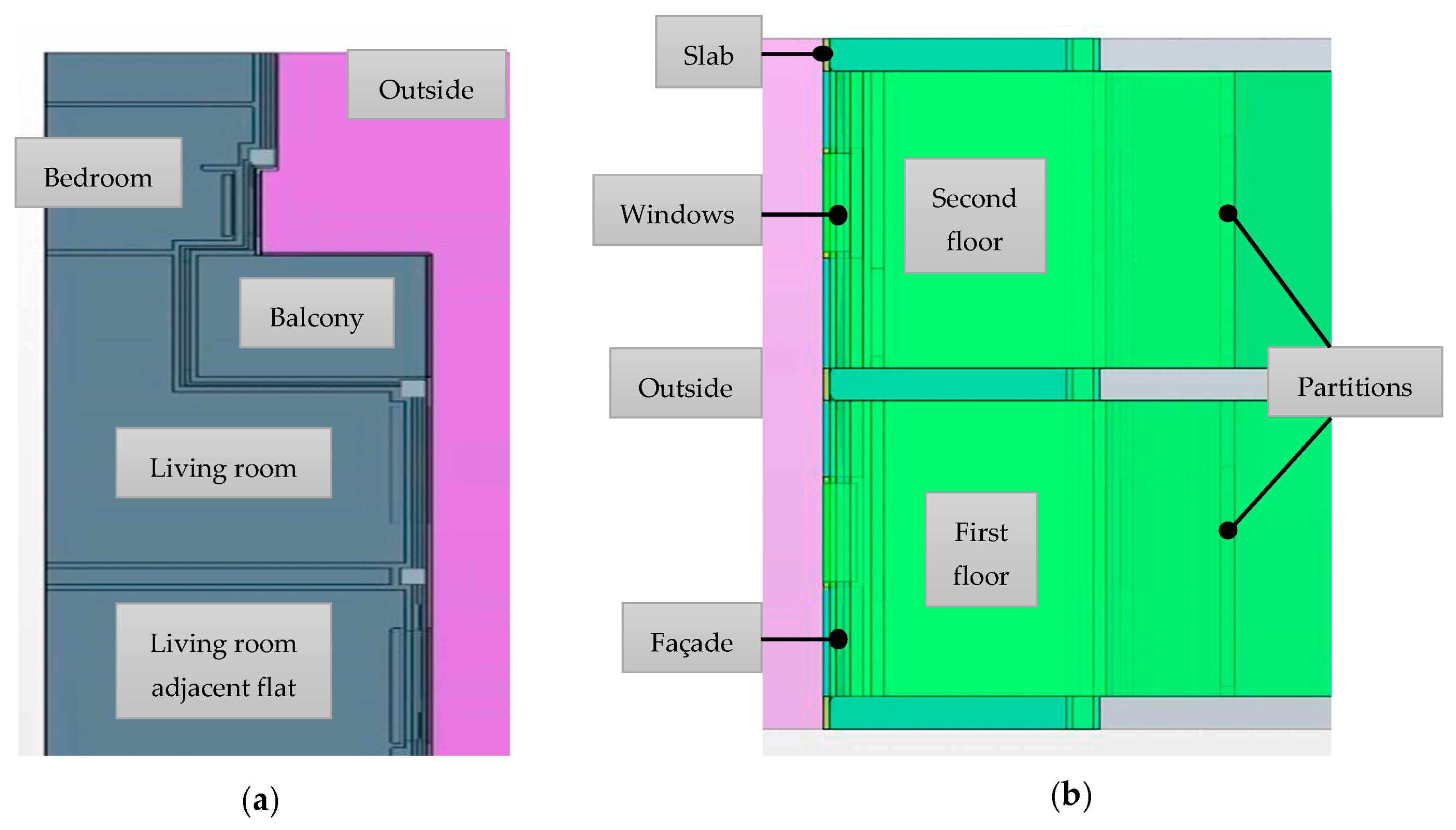
The house analysed in this research is situated in Hoyo de Manzanares (Madrid, Spain). It is a village in the mountains of Madrid (40°37′18″ N 3°54′33″ O), which has a predominant continental climate. Figure 1 shows interior layout plan of the house with different types of external walls and the analysed facade. The building was constructed in 1986 following the requirements of the standard NBE-79 [37], which is now repealed, without having received any interventions that improve its state during 30 years. The building is situated in the mountains of the Sierra of Madrid with latitude 40.39° N and longitude 3.47° O. The most important difference between current CTE DB-HE and already disused NBE-79 is that nowadays the levels of solar radiation are considered when different climatic zones are defined, taking into consideration location of the building and its internal charge while defining envelope thermal characteristics. When the studied building was constructed, only the loss through transmission via parameters was considered and thermal insulation recommendations were not mandatory for external walls.

2.2. Materials and Initial Energy Rating

Physical properties of building materials was obtained based on data collected from the construction project. These parameters were used to calculate thermal transmittance of different facade walls, used in the calculation of energy rating and modelling of the building. Project data is shown in

Table 2. Building materials properties.

Material	$\mathit{\rho }$ (kg/m3)	$\mathit{\lambda }$ (W/mK)	$\mathbf{c}$ (J/kg∙K)	Emissivity $\left(\mathit{\epsilon }\right)$	Reflectivity $\left(\mathit{\rho }\mathbf{G}\right)$	Transmissivity $\left(\mathit{\tau }\right)$
1/2 Foot face brick	780	0.35	1000	0.92	0.08	0.00
Cement mortar render	2000	1.50	960	0.92	0.08	0.00
Unventilated air chamber	1.20	0.024	1006	0.92	0.08	0.00
XPS Thermal insulation	50	0.035	150	0.92	0.08	0.00
Hollow brick partition	770	0.32	1000	0.92	0.08	0.00
Glass	2500	3.00	840	0.70	0.20	0.10
Gypsum plastering	750	0.30	1000	0.92	0.08	0.00
One-way slab	1140	0.85	1000	0.92	0.08	0.00

and

Table 3. Thermal transmittance through walls.

Vertical Walls					Horizontal Walls
Wall type	M1	M2	M3	M4	Wall type	Slab
UT (W/m2∙K)	0.41	0.40	0.56	0.59	UT (W/m2∙K)	0.85

.

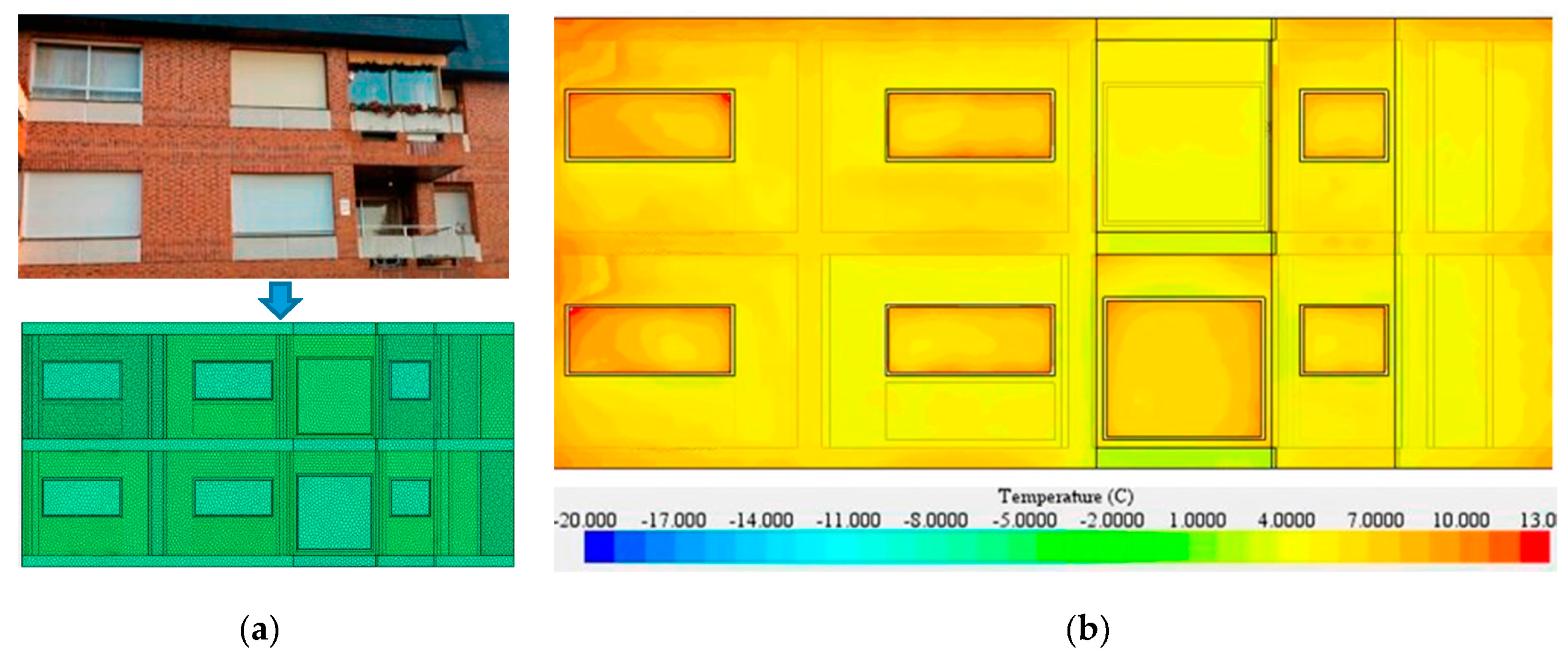
Once the composition of the walls was studied with the data collected from the actual state of the building, energy rating of the building was carried out using the CE3X v.2.3 [9] tool for residential buildings. To determine the energy performance of the building it was necessary to include the data of materials and transmittance through walls, the location of the building, a pattern of shadows of the facade and facilities of the building. The values of building elevation can be seen in Figure 2a, and the energy label obtained in the research is shown in Figure 2b, being this one the most common qualification for buildings based on the reference standard NBE-79.

2.3. Thermography

Thermography shows thermal radiation at determined wavelengths of analysed physical elements. This result is transformed into a numerical value that corresponds to its temperature by applying Stefan-Boltzmann’s Law, shown in Equation (1); as this equation is applied to a black body that emits all absorbed radiation, it does not work for the majority of surrounding objects (grey objects). In this way, a modified expression such as Equation (2) can be used, that takes into account the emissivity (ε) of a body in a way that the emissivity of a black body considered to be 1 and the emissivity of grey bodies considered to have a value between 0 and 1.

$$Q_{rad}=\sigma ·A_s·{\theta }_s^4\left(\mathrm{W}\right)$$

(1)

$$Q_{rad}=\sigma ·\epsilon ·A_s·{\theta }_s^4\left(\mathrm{W}\right)$$

(2)

Thermography shows images within a range of colours according to the pattern of each camera that corresponds to a number associated to each colour. For a correct interpretation of the results, the values have to be adjusted correctly, taking into consideration the recommendation of the standard UNE-EN ISO 7726 [38] for measuring microclimatic parameters it is possible to determine the indoor air temperature $\left(t_a\right)$ at which the image was taken.

This research was carried out using the first method, using a Ti90 camera (Fluke, Everett Washington, USA) with 4800 pixels resolution, thermal sensitivity $\le 0.15℃$ and measuring range from $-20℃$ to $250℃$. Moreover, it is needed to know the emissivity value of an object to take its thermography. For this reason, adhesive tape with $\epsilon =0.95$ was used and the photo was taken from the minimum distance in a way that its area includes completely the camera’s angle of vision. This previous data helps to interpret and assess correctly the obtained numerical data.

2.4. Experimental Conditions

Thermography images were taken on 17 March 2017 at 7:30 a.m. The studied facade has a west orientation, in a way that at dawn solar radiation does not impact the building directly, existing only a component of diffuse solar radiation. Environmental data was obtained in the micro climatic data logger located in the façade of the building. Heat transfer in the main direction of the facade and perpendicularly to it was considered. Taking as a calculation assumption the installed heating power system of the building, the power of the unit heaters was calculated according to the standard UNE-EN ISO 13790 which describes the calculation of the energy demand of heating [39]. The calculation method is expressed mathematically by Equations (3)–(6):

$$Q_{Total}=Q_{Trans}+Q_{Vent}\left(\mathrm{W}\right)$$

(3)

The heat transfer variables can be obtained in the following way:

$$Q_{Trans}=\left({{\displaystyle \sum }}^{\text{}}{A}_i·U_i+l_k·{\psi }_k\right)·\left({\theta }_{int,set}-{\theta }_e\right)\left(\mathrm{W}\right)$$

(4)

$$Q_{Vent}=H·\left({\theta }_{int,set}-{\theta }_e\right)\left[\mathrm{W}\right]$$

(5)

Moreover, the value of $H$ can be obtained using the following expression:

$$H={\rho }_a·c_a·Q_{vent}\left(W/K\right)$$

(6)

The flows described in the CTE DB-HS3 were used for the minimum required ventilation flows in bedrooms and living rooms [40], without taking into consideration the infiltrations in the analysed model. As in the moment when thermography was taken the heating was switched on,

Table 4. Experimental conditions.

Area	Initial Conditions	Other Parameters
Bedroom 1	Heater supplied energy: 646 $\mathrm{W}$	Key temperature: 20 $℃$
Living room	Heater supplied energy: 1053 $\mathrm{W}$	Ambient temperature: $-0.1℃$
Living room of adjacent flat	Heater supplied energy: 458 $\mathrm{W}$	Direct radiation: $0\mathrm{W}/{\mathrm{m}}^2$
		Diffuse radiation: $10\mathrm{W}/{\mathrm{m}}^2$

shows initial conditions for thermal modelling in terms of heat power in every room, as well as solar radiation parameters which correspond to the moment of measuring.

2.5. Geometric Model

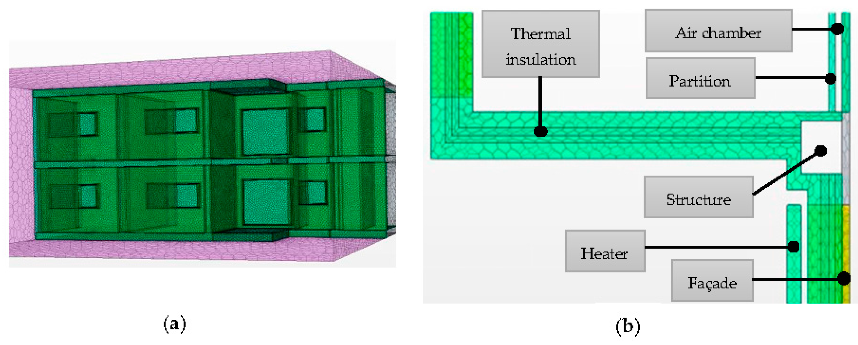
To define the geometry used in the numeric simulation model, real dimensions of the building were taken as a reference. Moreover, to optimize calculation time in building simulation, thickness of objects are multiples of 5 cm and dimensions of the model were adjusted in CAD until a unified size was obtained for all the areas. Mesh was refined making it denser with smaller cells close to the facade of the building and in the windows, as well as in heaters and in the interfaces between different areas of the plan. Moreover, layers of air of 2 cm thickness were included in interior and exterior areas of the facade, in order to simulate correctly heat transferred through the solid surface of the facade in contact with flows that involve it through convection.

Figure 3 shows the geometric definition of the model that corresponds to the first two floors of the real building. To choose the size of the cells of the mesh of each area, the error depending on different mesh sizes was calculated. For this, investigations validated by Roache [41] were taken as a reference for simulation in CFD programs. This paper proposes the value of Grid Convergence Index (GCI) to quantify the error corresponding to the mesh size which provides the objective value that quantifies uncertainty in the model based on error estimation produced after mesh refining. The equations to calculate GCI are expressed as follows:

$$GCI=\frac{F_s\left|E\right|}{\left(1-r^p\right)}$$

(7)

$$E=\frac{f_c-f_f}{f_f}$$

(8)

$$r=\frac{h_c}{h_f}$$

(9)

Thus, it deals with finding asymptotic value at which different mesh sizes converge. The security factor $\left(F_s\right)$ reduces range error produced in approximation between refined solution $f_c$ and unknown exact solution $f_f$, which is fixed in the value $F_s=3$. The difference between the original size of cells $h_c$ and refined size $h_f$ is related through coefficient $r$, as it is shown in Equation (9). Recommended values for $r=p=2$.

The study of cells size was carried out on partial section of the facade due to the big size of the model as a whole. Thus, the obtained error between selected cells size and cells that are two or five times smaller is of 1.05% and 1.34%, respectively, which can be considered as negligible assuming proposed mesh values for the modelling, reducing in this way the model calculation time.

Furthermore, it was decided to use polyhedral model in order to avoid errors produced in the surface common in the succession of layers of different material that form the enclosures, taking as a basis 5 cm mesh for all the areas. In case of areas of transfer between different objects, the size of the mesh was reduced with the use of two prismatic layers of 1 cm thickness, reducing in this way the error and refining the model in order to obtain higher continuity in stationary flow of heat between interior and exterior part of the building. Different types of the mesh used in the modelling are shown in

Table 5. Mesh model.

Body	Type of Cells	Mesh Size (cm)
Ambient air	Polyhedric	5
Inner and unventilated chamber air	Polyhedric	5
Solid bodies	Polyhedric	5
Interfaces	Ortogonal (Prism layer)	Two layers of 1 cm each one

, indicating the corresponding area.

The simulated model is centered on the first and the second floor of the building, which are 14 m long and 7 m and 6 m high, respectively, as it can be observed in Figure 4. As a whole, the mesh used is composed by more than two million cells.

The comparison of the thermography taken in situ with the CFD modelling program was carried out as accurately as possible, imitating the process of building construction, taking into consideration the materials used in the original construction. This research used as a model of finite element simulation the Star-CCM+ 8.05.006 program [42]. This program was used in numerous studies related with building for the modelling of natural ventilation in the enclosures [43,44], and for observing the thermal performance of building envelopes under different constructive solutions [45,46].

In order to analyse the thermal performance of the simulated building, boundary conditions were fixed allowing one to set differential equations that are resolved in modelling, indicating values of physical variables that allow comparing thermography with computational analysis. The simulated model is composed of 61 different zones according to the material, for this reason the values of corresponding physical parameters were taken into consideration for each one. Furthermore, some of the parameters were considered common for all of them, such as the gravity and the stratification of air flow, what was applied to movements of vertical convection in a condition of boundary between the facade and the air.

Heat flow transfer in stationary state between interior and exterior part of the building was calculated using Fourier’s Law for the conduction between different solids being in contact (Equation (4)) and Newton’s Law for the solid surfaces in contact with flows at different temperature (Equation (5)).

To simulate convective heat transfer, a model of approximate turbulence defined by the equations of Reynolds-Averaged Navier-Stokes (RANS) was used, obtaining instantaneous velocity and pressure decomposed to an average value and a fluctuating component in conditions of stationary balance. In particular, the effect of the turbulence has been defined using the Realizable k-epsilon model, validated in other studies to calculate natural convection flow [47,48].

Boundary conditions are the internal and external temperature. The air is modelled as an incompressible ideal gas. The effect of the gravitational forces is also included. The walls of the exterior volume air have been set to the external temperature. Moreover, the walls of the inner air volume have been set to the key temperature of the building. The heat transfer model analysed includes conduction, convection and radiation. In the specific case of heat transfer by radiation, a model surface to surface was used. This model is valid for explication of exchangeable radiation in area of diffuse grey surfaces. Thus, energy exchange between both surfaces depends partially on its size, distance of separation and orientation, being those the factor counted by so called view factor [49].

3. Results

Evaluation of the current state of the building according to CFD modelling is shown in Figure 5. General evaluation of thermal bridges through facade can be observed, especially in the intersections between the vertical parameters with horizontal structure of slabs.

Lack of insulation in these areas causes higher loss of heat per unit of surface that is reflected in the model in accordance with the predictions done for the real building.

3.1. Thermography Analysis

Thermographic images of the facade show thermal bridges in slab edges and pillars of the facade (Figure 6), as it can be seen in CFD modelling. A change of colour also can be observed under the windows, associated with an approximate temperature difference of 5 °C with respect to the rest of the facade where the average temperature is 3.5 °C. This variation corresponds with the location of heaters.

Deepening the analysis of the thermography, it can be observed how the exterior wall of the facade is made with different materials. On one side, first two floors are made with brick, a rough and opaque material with emissivity close to 1, which is represented by a warm colour (Figure 6a). On the other hand, the last floor has a smooth slate finish that increases its reflectivity (Figure 6b); additionally its inclination is not vertical, what leads as a result in the thermography of the reflected sky temperature, explaining the difference between the demonstrated temperature and the brick wall temperature. Thus, brick temperature is closer to the reality, while slate temperature does not show reliable emissivity values and, consequently, it was discarded in the CFD model.

3.2. Validation of the CFD Model

The CFD model, that analyses different physical values in stationary state, was constructed using the characteristics established in the previous subsections. The validation was carried out through observation of phenomena highlighted in the thermography. Starting from the facade (Figure 7), as it can be observed that the CFD images become much more homogeneous without low temperature values, if we exclude the upper floor from the study.

Moreover, thermal bridges caused by lack of insulation around the structure are shown in the CFD image with a similar value to the one obtained by the thermography camera. The variation of the temperature values in the areas of the heaters and the convection air flow due to different density are also shown, reaching similar temperature values using both methods. For its validation through external part of the facade, three points were analysed using thermography and the CFD model. In these points, the difference between average temperatures varies between 0.6 °C and 0.8 °C, being this difference lower than the precision of the thermographic camera making the error negligible.

4. Discussion

Once the numerical model of the building in 3D is obtained, it is possible to carry out a deeper analysis of its performance and to evaluate possible improvement suggestions. Beyond the results shown in Figure 5 and Figure 7, where the lack of thermal insulation in vertical and horizontal walls can be seen emphasizing in this way thermal bridges, lack of double glazing and temperature gradients produced by natural convection inside the building, the given initial conditions should lead to a habitability result inside the building, which is analysed in Figure 8. The temperature obtained in the interior areas corresponds to similar values of the key temperature established inside the building $\left(\approx 20℃\right)$. The hottest areas correspond to the vertical projection of the heaters, as happens in reality. The ambient temperature is the same as the reference taken from the micro-climatic data logger $\left(0.1℃\right)$.

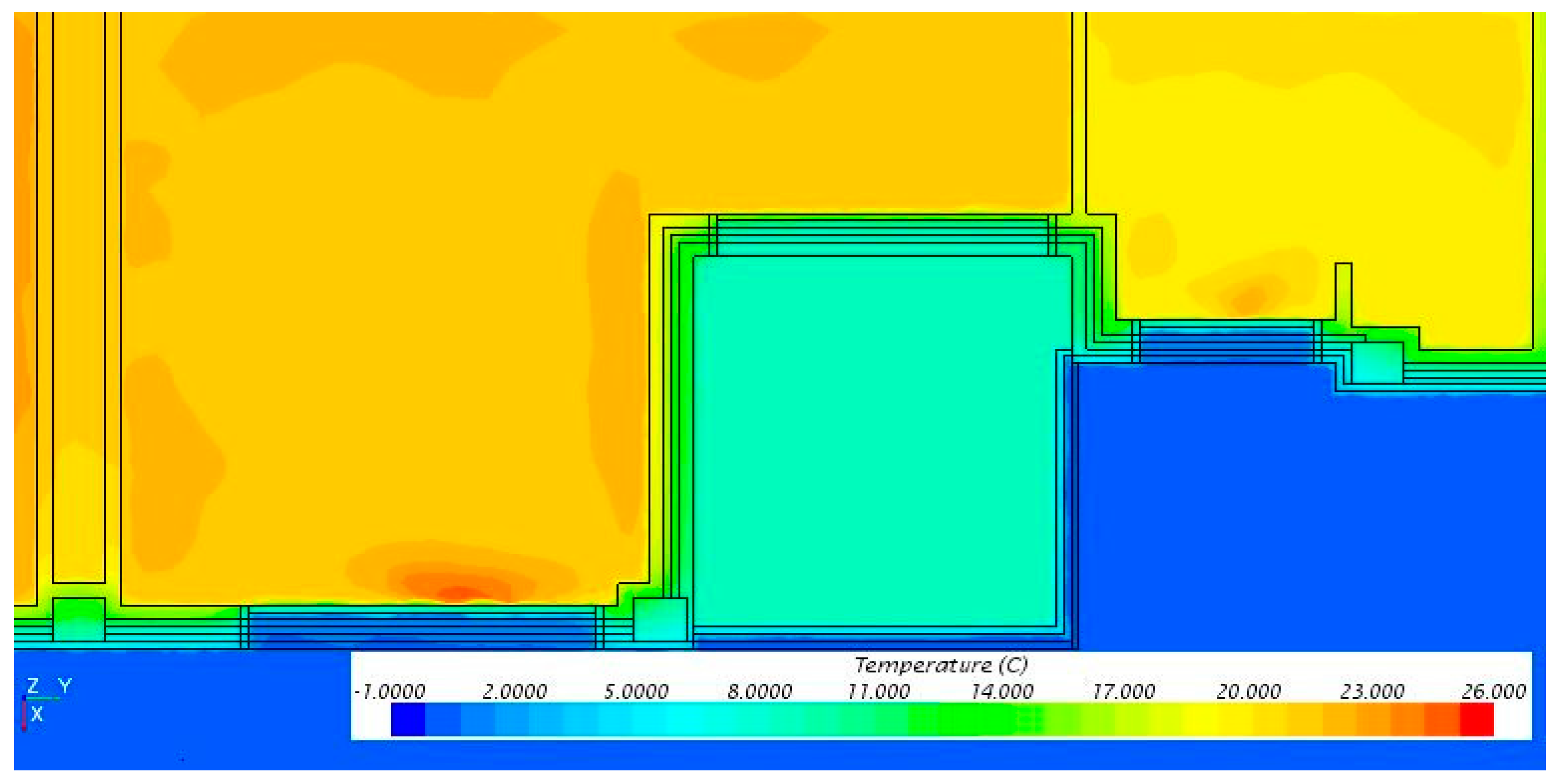
On the other hand, Figure 9 shows in detail the horizontal section of the second floor, being reached values in the interior areas $1.5℃$ higher than that of the lower floor. Air confined in the balcony is about $10℃$, absorbing the influence of the outside ambient temperature and reducing the energy consumption of the house.

Analysing other plans of the building, different from the facade, Figure 9 shows the vertical section of the building where it can be seen how the thermal bridge extends through the entire structural element because of lack of insulation in its outer slab front. The upper temperature range was limited to $25℃$, that is why the areas that surpass this value are white. The temperatures of the heaters in the model reach $50℃$, coinciding with the usual temperature of the heating supply boiler temperature in the building, according to the current standard RITE-2013. Because of the lack of insulation, all the slabs act as thermal bridges, lower temperatures being observed in their exterior faces, while interior air becomes stratified responding to the gravitational behaviour according to which hotter flows ascend (Figure 10).

Global and Local Comfort Assessment

This kind of CFD programs also allows analysis of the thermal comfort of the residents. The standard UNE-EN ISO 7730 [50], relates thermal sensation with thermal balance, which depends on the physical activity, clothing of a subject, and other environmental parameters (air temperature, meant radiant temperature, air velocity and relative humidity). Thermal sensation can be estimated through Predicted Mean Vote (PMV) calculation and Predicted percentage of dissatisfied (PPD) index, which is defined from the PMV [50]. The PMV is expressed mathematically as described in the (10) and develops as follows in the Equations (11)–(13). The calculation of PMV index has been integrated in the Star-CCM+ simulations taking special care of all input variables required in Equations (10)–(13) as recently stressed by d’Ambrosio Alfano et al. [51,52]. In this way, all errors which affect also robust commercial tools have been minimized:

$$\begin{array}{l}PMV\\ =\left[0.303·\exp \left(-0.036·M\right)+0.028\right]\\ ·\left\{\begin{array}{c}\left(M-W\right)-3.05·{10}^{-3}·\left[5733-6.99·\left(M-W\right)-p_a\right]-0.42·\left[\left(M-W\right)-58.15\right]\\ -1.7·{10}^{-5}·M·\left(5867-p_a\right)-0.0014·M·(34-t_a)\\ -3.96·{10}^{-8}·f_{cl}·\left[{\left(t_{cl}+273\right)}^4-{\left(\overline{t_r}+273\right)}^4\right]-f_{cl}·h_c·\left(t_{cl}-t_a\right)\end{array}\right\}\end{array}$$

(10)

$${\theta }_{cl}=35.7-0.028·\left(M-W\right)-I_{cl}·\left\{\begin{array}{c}3.96·{10}^{-8}·f_{cl}·\left[{\left(t_{cl}+273\right)}^4-{\left(\overline{t_r}+273\right)}^4\right]\\ +f_{cl}·h_c·\left(t_{cl}-t_a\right)\end{array}\right\}$$

(11)

$$h_c=\left\{\begin{array}{c}2.38·{\left|t_{cl}-t_a\right|}^{0.25}for2.38·{\left|t_{cl}-t_a\right|}^{0.25}>12.1\sqrt{v_{ar}}\\ 12.1\sqrt{v_{ar}}for2.38·{\left|t_{cl}-t_a\right|}^{0.25}<12.1\sqrt{v_{ar}}\end{array}\right\}$$

(12)

$$f_{cl}=\left\{\begin{array}{c}1.00+1.290I_{cl}for{I}_{cl}\le 0.078{\mathrm{m}}^2·\mathrm{K}/\mathrm{W}\\ 1.05+0.645I_{cl}for{I}_{cl}\ge 0.078{\mathrm{m}}^2·\mathrm{K}/\mathrm{W}\end{array}\right\}$$

(13)

Experimentally, the PMV value is obtained for a determined measurement point and the results are extrapolated to the studied area. However, the use of CFD simulation programs allows one to calculate PMV for each cell of the mesh used in the calculations. Metabolic rate was estimated according to the UNE-EN 7730 standard, taking into consideration that elderly persons often have lower activities compared to young persons. In this case, sedentary activity with average metabolic rate of 70 $\mathrm{W}/{\mathrm{m}}^2$ was considered for one person. Moreover, basic clothing insulation value of 1.0 clo was taken into account for calculations in winter season. Taking into account all closed openings in the moment of simulation, there is no considerable air flow inside the room, so a value of 0.05 m/s for $v_a$ was considered according to the standard UNE EN ISO 7730. Mean radiant temperature $\overline{T_r}$ was calculated based on surface temperature of surrounding surfaces as indicated in the standard UNE-EN ISO 7726, assuming that temperature of opaque elements coincides with the air temperature due to high emissivity of building materials. For this, the Equation (14) established by the standard is used:

$${\overline{T_r}}^4=T_1{}^4·F_{p-1}+T_2{}^4·F_{p-2}+\dots +T_N{}^4·F_{p-N}$$

(14)

where $\overline{T_r}$ is mean radiant temperature in K, $T_N$ is N surface temperature, in K and $F_{p-N}$ is a factor of form between one person and N surface.

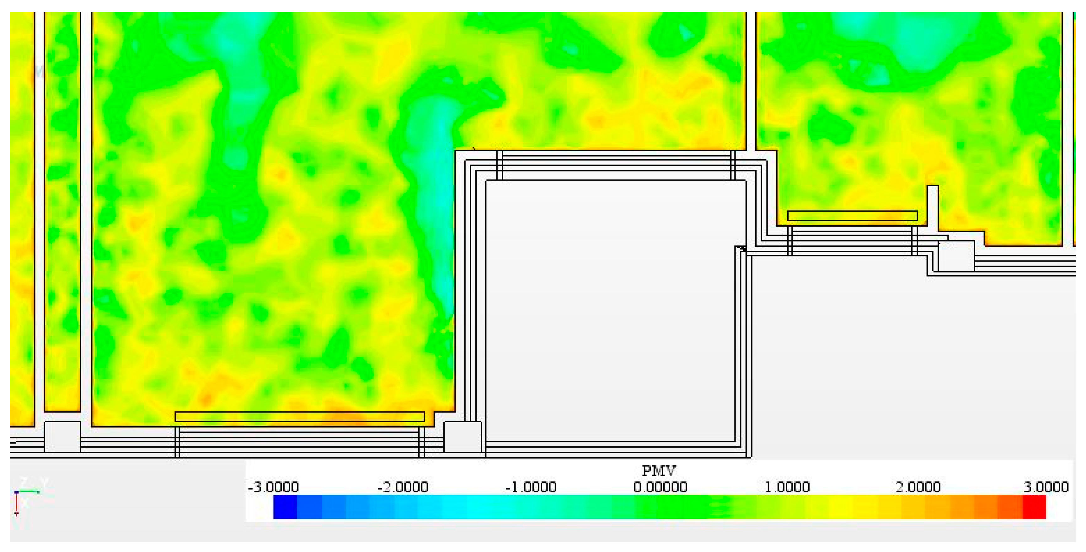
The results obtained in the analysis of the thermal comfort are shown in Figure 11, where it can be observed that the values vary inside each area according to the previously described variables. The values of 0.7 in the living room and 0.6 in the bedroom are obtained applying one measure to each represented surface. These values correspond to a slightly hot thermal sensation in the interior of the house, listed in the class C according to the standard UNE-EN 7730 that indicates dissatisfaction rates due to different considered factors global thermal discomfort.

However, asymmetry of radiant temperature can cause discomfort, for this reason this factor has been taken into consideration in the worst case considering the façade as a cold wall that according to the standard UNE EN ISO 7730 is indicated by:

$$PD=\frac{100}{1+exp\left(6.61-0.345·\Delta t_{pr}\right)}$$

(15)

where $PD$ is the percentage of unsatisfied (%), and $\Delta t_{pr}$ is the asymmetry of radiant temperature ($℃)$.

In the given CFD model, the average temperature of each surface was obtained using mean value in each boundary. For the studied building, the living rooms of both houses present differences, as on the floor 1 the balcony is open to the exterior, when on the floor 2 there is a second line of window on the external edge of the balcony what makes it closed. As it can be seen in

Table 6. PD temperatures and values obtained in living rooms of both studied floors.

Living Rooms	Average Temperature of the Inner Side of the Window $(℃)$	Average Temperature of the Opposite Wall $(℃)$	Percentage of Dissatisfied PD (%)
Floor 1	8.9	18.1	3.1
Floor 2	14.8	20.0	0.8

, the difference between temperatures of both areas provokes the minor percentage of unsatisfied inhabitants on the floor of closed balcony.

It is necessary to indicate the importance of the works of Povl Ole Fanger focused on the investigation of parameters that affect indoor air quality and can be used even nowadays as a reference in performing researches of this type [53]. In particular, in PMV parameters calculation, there is a great amount of applications both free and commercial. However, not all of them provide reliable results that can be used in building projects [54], that gives an additional value to this simulation with Star-CCM+ that allow treating this thermal comfort parameter with a high level of precision. Some authors such as Gan [55], already used more than two decades ago the calculation of comfort index to evaluate distribution of air inside an area. More recently, Gao et al. [56,57], used PMV calculation in the study of radiant cooling system and thermal comfort associated to its use; performing simulations for different temperature conditions in spite of the asymmetry presented in some cases, with an aim to optimize the design of the building. Other authors such as Huan et al. [58], calculated PMV index obtaining good results for the simulation of stratified ventilation in offices using highly asymmetric gains of heat.

Thus, the use of CFD programs in the calculation of thermal comfort allows one to deepen and calculate thermal sensation in each point calculated by the mesh volume instead of considering it uniform throughout all the area, as it is done experimentally. Moreover, the use of this type of tool allows optimal evaluation of improvement suggestions without acting on analysed building. Analysed improvement suggestion as an example consists in filling the actual air chamber with thermal insulation with density of 30 $\mathrm{kg}/{\mathrm{m}}^3$ and thermal conductivity of 0.035 W/(m K), with the aim to reduce the loss of energy through the facade reducing the thermal bridges of the building.

As this evaluation is stationary at a particular moment, the same calculation procedure was carried out for the heaters power followed in the Section 2.4, in other words, the Equations (3)–(6) and data of Table 3 were taken into consideration. Theoretical calculation of the heaters power turns out to be 11% lower—over the values shown in Table 2—than in the current state, what allows optimization of energy consumption.

The results obtained using the CFD model is shown in

Table 7. Results obtained through the CFD model.

Subject	Current State		Improves Suggestion and 11% Less Power of Heaters		Improves Suggestion and Heaters with Actual Power
Building	Living Room Mean Air Temperature $(℃)/\mathrm{PMV}$	Bedroom Mean Air Temperature $(℃)/\mathrm{PMV}$	Living Room Mean Air Temperature $(℃)/\mathrm{PMV}$	Bedroom Mean Air Temperature $(℃)/\mathrm{PMV}$	Living Room Mean Air Temperature $(℃)/\mathrm{PMV}$	Bedroom Mean Air Temperature $(℃)/\mathrm{PMV}$
Floor 2	21.7/1	20.0/0.75	21.6/1	19.8/0.7	22.7/1.16	21.1/0.91
Floor 1	20.2/0.75	19.2/0.62	20.1/0.77	19.0/0.6	21.2/0.92	20.3/0.79

, where the temperatures of the rooms and the thermal sensation of the residents can be also observed. Comparing all these results, it can be observed that after improvements and maintaining the heaters power the temperature and thermal sensation increase. If on the contrary, both parameters (temperature and thermal sensation) maintained fixed, the reduction of 11% of energy used by heaters is obtained, what increases at the same rate saving of a user and energy efficiency.

5. Conclusions

The thermography analysis of the building’s facade allowed a comparable 3D numerical model using a CFD modelling tool, obtaining a similar thermal performance with both methodologies. In both techniques the influence of the lack of insulation on the heat loss through the facade can be observed. Moreover, CFD model allows to correct the temperatures that are in such elements of high reflectivity as glass and slate are incorrect in the thermography, being opaque material those that have to be considered to validate the comparison of two methodologies.

Global difference between measures with thermographic camera and those obtained by modelling for the same points varies between 0.6 °C and 0.9 °C. Thus, the interior temperature in studied areas in the CFD model varies by 1 °C maximum with regard to the real average temperature in the building. That is why both levels of error are under the precision of measuring elements used for the in situ tests, being therefore comparable the results obtained by modelling with thermography images.

Moreover, CFD analysis allows, contrary to infrared thermography, assessing the influence of each material of facade and its envelope, providing in such a way more information. Therefore, it is possible to evaluate during rehabilitation the influence of different energy saving measures on the building. As an example, an improvement can be observed when the air chamber is replaced by the projected thermal insulation allowing a reduction of the energy demand of the building by 11%.

Another advantage over visual inspection techniques and experimental measures, is that the use of modelling programs such as Star-CCM+ makes it possible to evaluate the thermal comfort of the building allowing one to perform quantitative analysis of thermal comfort in the studied area. In particular, a 0.6 value was obtained in the PMV index calculation, which classifies the house as C class according to the UNE EN ISO 7730 standard. This value adds a significant value to the research as European legislation indicates that energy efficiency of a building has to be guaranteed taking into consideration the thermal comfort of inhabitants, being necessary to complete rehabilitation works with a prediction in terms of indoor comfort before starting any installation.