Article

Adaptive Feedback Linearization Based NeuroFuzzy Maximum Power Point Tracking for a Photovoltaic System

1
Department of Electrical Engineering, COMSATS Institute of Information Technology, Abbottabad 22060, Pakistan
2
Department of Electrical and Electronics Engineering, Faculty of Engineering, Sakarya University, Serdivan 54050, Sakarya, Turkey
3
Department of Electrical Engineering, Higher Polytechnic School of Algeciras, University of Cadiz, 11202 Algeciras, Spain
4
Department of Power System and Its Automation, Chongqing University, Chongqing 400044, China
*
Author to whom correspondence should be addressed.
Energies 2018, 11(3), 606; https://doi.org/10.3390/en11030606
Submission received: 17 January 2018 / Revised: 1 March 2018 / Accepted: 6 March 2018 / Published: 9 March 2018
(This article belongs to the Special Issue Sustainable and Renewable Energy Systems)

Abstract

:
In the current smart grid scenario, the evolution of a proficient and robust maximum power point tracking (MPPT) algorithm for a PV subsystem has become imperative due to the fluctuating meteorological conditions. In this paper, an adaptive feedback linearization-based NeuroFuzzy MPPT (AFBLNF-MPPT) algorithm for a photovoltaic (PV) subsystem in a grid-integrated hybrid renewable energy system (HRES) is proposed. The performance of the stated (AFBLNF-MPPT) control strategy is approved through a comprehensive grid-tied HRES test-bed established in MATLAB/Simulink. It outperforms the incremental conductance (IC) based adaptive indirect NeuroFuzzy (IC-AIndir-NF) control scheme, IC-based adaptive direct NeuroFuzzy (IC-ADir-NF) control system, IC-based adaptive proportional-integral-derivative (IC-AdapPID) control scheme, and conventional IC algorithm for a PV subsystem in both transient as well as steady-state modes for varying temperature and irradiance profiles. The comparative analyses were carried out on the basis of performance indexes and efficiency of MPPT.

1. Introduction

The grid-integrated photovoltaic (PV) system is sequentially being followed as a supplement and an alternative energy source to the conventional fossil fuel generation in order to fulfill the increasing energy demand and to overcome the adverse environmental issues caused by fuel emissions [1]. PV is considered as the most promising and reliable energy source because it is clean, pollution-free, and abundantly available [2]. The fundamental concern of PV generation is that its output power is reliant on the atmospheric conditions. On the P-V curve, only one point exists where the PV output power is the maximum. To track the maximum power point (MPP) at all environmental conditions, an efficient maximum power point tracking (MPPT) technique is required which forces the PV to operate at that MPP. MPPT is quite a crucial part of the PV system.
A number of conventional and advanced MPPT schemes have been stated in the literature. The conventional techniques include perturb and observed (P&O) [3], incremental conductance (IC) [4,5], fractional open circuit voltage (OCV) [6], fractional short circuit current (SCC) [7], and the ripple correlation method (RC) [8]. Although conventional techniques are simple and most commonly used, they have certain limitations which cannot be ignored. P&O and IC MPPT techniques are slow and oscillate around MPP. OCV and SCC have a low efficiency and accuracy. The RC method is quite complex to implement. The advanced MPPT methods involve the artificial neural network (ANN) [9], fuzzy logic [10], meta-heuristic algorithms [11,12], and the feedback linearization method [13]. Although ANN provides accurate MPP, it has to be periodically trained for the specific PV system with which it is utilized. Fuzzy logic MPPT performs well under fluctuating meteorological conditions. However, its performance depends a lot upon the prior knowledge of the system input/output relationship. Whilst meta-heuristic algorithms are successfully applied to track the MPP under a non-uniform irradiance level, their convergence speed, suitable selection of control parameters, and solution archive need significant attention. The feedback linearization approach is a new MPPT method for the grid-connected PV system [14]. The grid-integrated PV system has a nonlinear state model. Therefore, the input/output linearization method is a more suitable solution to acquire the MPP of the grid-connected PV system. Feedback linearization initially converts the nonlinear system into entirely or moderately decoupled linear subsystems and then implements the renowned linear control laws on these subsystems [15]. Feedback linearization control is broadly used for large classes of nonlinear systems, e.g., high voltage direct current (HVDC) links [16], electrical motors [17], PWM rectifiers [18], and robotics [19]. However, feedback linearization control has a limited region of stability and lack of robustness to un-modeled system dynamics [20]. These drawbacks of classical feedback linearization have been eliminated by using the adaptive feedback linearization-based NeuroFuzzy algorithm for uncertain nonlinear systems [21]. A NeuroFuzzy is basically a fuzzy system in which the learning algorithm for training is inspired by ANN [22,23]. So, NeuroFuzzy amalgamates the explicit knowledge of fuzzy logic, which is analyzed and inferred with the implicit knowledge of ANN that is obtained by learning [24,25]. Moreover, the adaptive control is able to deal online with system nonlinearities, uncertainties, and fluctuations [26,27,28]. Therefore, in an adaptive feedback linearization-based NeuroFuzzy algorithm, the uncertain nonlinear system is initially identified using the NeuroFuzzy inference system and then adaptive feedback linearization is capable of controlling the identified nonlinear system [29].
In this paper, an adaptive feedback linearization-based NeuroFuzzy (AFBLNF-MPPT) technique for a PV subsystem in a grid-integrated hybrid renewable energy system (HRES) is proposed. In the proposed HRES, tracking the MPP is an extremely challenging issue, because the PV subsystem is intensely characterized by nonlinearity. The nonlinearity appears due to the intermittent solar radiation and dynamic temperature.
The rest of the article is arranged into four main sections. Section 2 provides a brief description HRES configuration and problem formulation. Section 3 provides details of the adaptive feedback linearization-based NeuroFuzzy MPPT (AFBLNF-MPPT) for a PV subsystem. Simulation results are presented in Section 4. Section 5 concludes this research work.

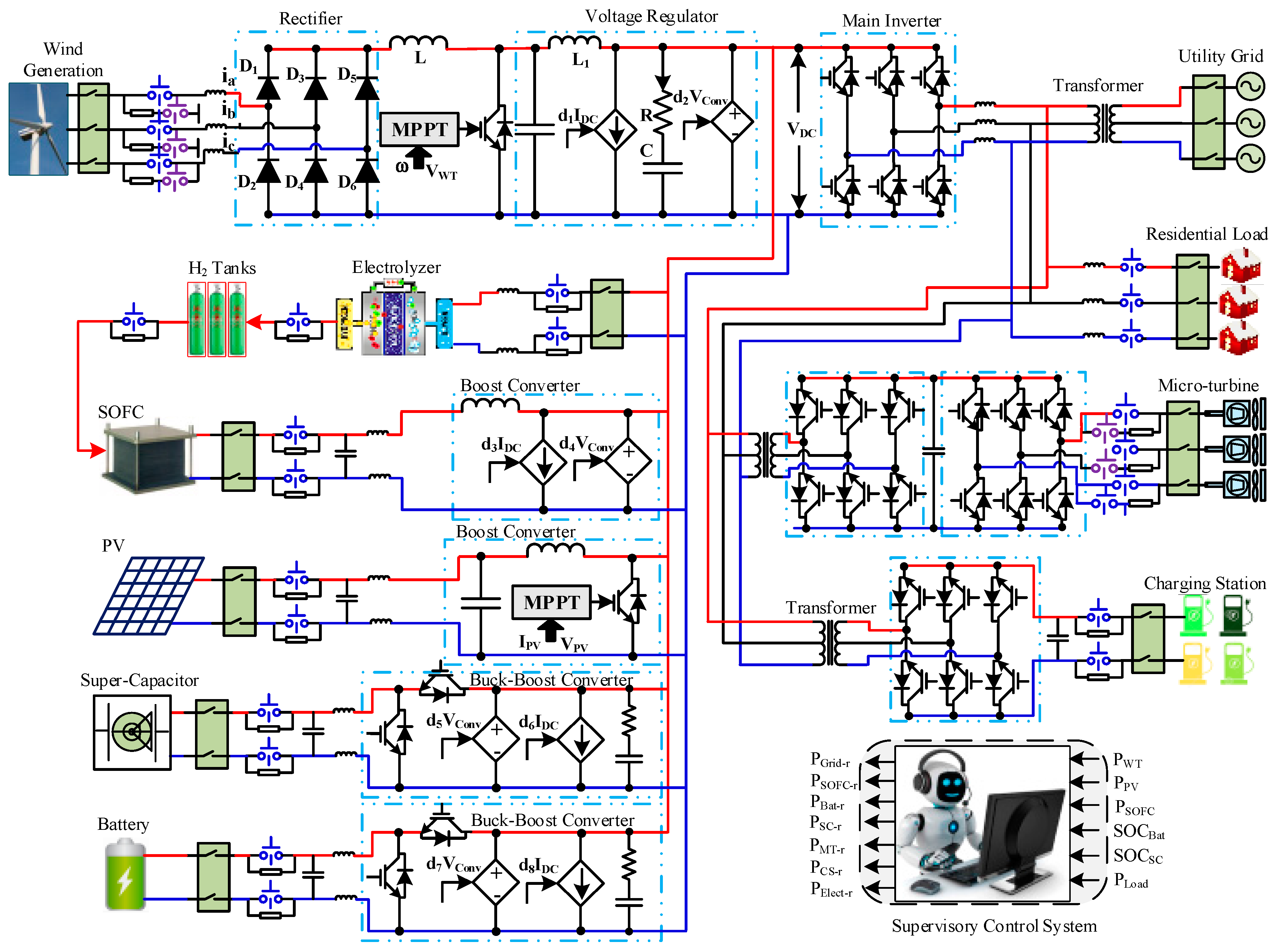
2. HRES Configuration and Problem Formulation

The HRES consists of a wind-turbine (WT), PV, solid oxide fuel cell (SOFC), electrolyzer, micro-turbine (MT), battery, super-capacitor (SC), and utility grid (UG) as sources, while the residential load and plug-in hybrid-electric vehicles (PHEVs) based charging station (CS) load are considered as the total demand [22].
In the stated HRES, the MPP from WT is extracted using an indirect adaptive NeuroFuzzy MPPT control scheme [22]. The load following problem of SOFC is resolved using an indirect adaptive NeuroFuzzy control scheme [22]. The WT, PV, SOFC, electrolyzer, battery, and SC are integrated to the DC-side, whereas UG, MT, CS, and residential loads are integrated to the AC-side. The grid side inverter (GInv) connects the DC-side to the AC-side, as shown in Figure 1. All the converters used in HRES are controlled by AdapPID.

Problem Formulation

The auto-regression NeuroFuzzy model of the nonlinear single-input-single-output (SISO) PV subsystem is represented as:
y ^ = f ( Ω ) = f ( y ( t 1 ) ,   ,   y ( t n ) ,   u ( t ) ,   u ( t 1 ) ,   ,   u ( t m ) )
where t represents the number of iterations; y = s is the slope of PV power w.r.t the operating voltage and y ^ = s ^ is the predictive output, i.e., the predictive slope of PV power w.r.t the operating voltage; and u represents the control input. The nonlinear dynamic model for a PV subsystem is caught online if:
l i m t   Ξ I d e = l i m t [ y y ^ ] ε I d e
where ε I d e is the identification error. The control law for a PV subsystem can be written as:
u M P P T = g A F B L N F M P P T ( y ,   y r e f )
where y = s is the actual output PV subsystem, y r e f = s r e f is the reference trajectory, and g A F B L N F M P P T represents the nonlinear function. Equation (4) is used to track the refernce trajectory of the PV subsystem for all t [ 0 ,   ] as:
l i m t   Ξ C o n t = l i m t [ y y r e f ] e C o n t
where e C o n t is the controller’s small tracking error. The MPP of the PV subsystem is achieved when the slope of PV power w.r.t the operating voltage becomes zero, as follows:
s | M P P = P P V V P V | M P P = 0
s | M P P = P P V V P V | M P P = ( I P V × V P V ) V P V | M P P = [ I P V V P V V P V + V P V I P V V P V ] M P P = [ I P V V P V + I P V V P V ] M P P = 0
s.t. (PV subsystem model constraints)
lim t { s ^ s s s r e f V P V V M P P P P V P M P P
where P M P P is the MPP of the PV subsystem, V M P P is the MPP voltage, and I M P P is the MPP current. The dynamic input conductance and the negativity of the static input conductance are the same at MPP for the PV subsystem. The impedance that appears at the input of the boost converter depends upon the duty cycle variation.

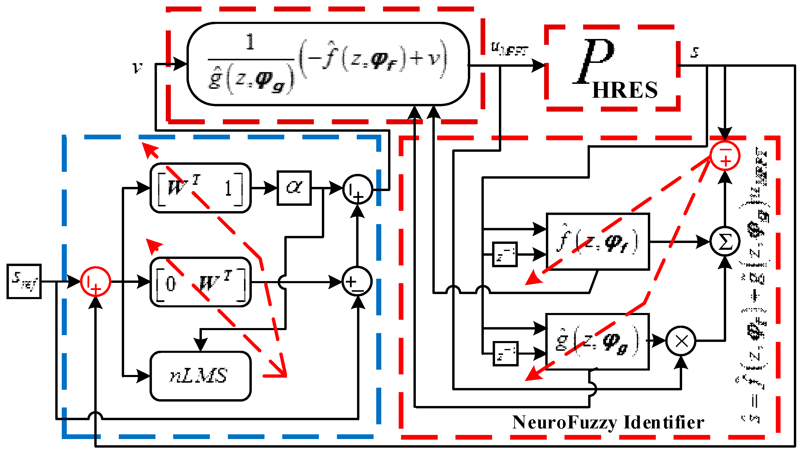
3. Adaptive Feedback Linearization Based NeuroFuzzy MPPT for PV Subsystem

3.1. Adaptive Feedback Linearization Control Law Design

The SISO PV subsystem of nth order is represented as follows:
z ˙ n = f ( z ) + g ( z ) u M P P T
where z n is a state variable, u M P P T m is a control input variable, and f ( z ) n and g ( z ) n × m are unknown nonlinear functions of the state vector with f ( 0 ) = 0 and g ( z ) > 0 . The SISO system is defined as follows:
y = z 1 ,   z ˙ 1 = z 2 ,   ,   z ˙ n 1 = z n
where y m is the output variable. An SISO system can be represented by a companion form after n-times by differentiating the y as follows:
y n = f ( z ) + g ( z ) u M P P T
The prime objective of feedback linearization control is to design the control law u M P P T to operate the PV subsystem on a reference trajectory y r e f with an acceptable accuracy. The output of the PV subsystem and reference trajectory is defined as follows:
z = [ y ,   y ˙ ,   ,   y n 1 ] T
z r e f = [ y r e f ,   y ˙ r e f ,   ,   y r e f n 1 ] T
A state error vector is calculated as:
e C o n t = [ y y r e f ,   y ˙ y ˙ r e f ,   ,   y n 1 y r e f n 1 ] T
or
e C o n t = [ e C o n t   e ˙ C o n t   ,   e C o n t n 1 ] T
The dot product of the weight vector and error vector is called filter tracking error, which is given as:
ϒ T = [ w 1 ,   w 2 ,   ,   w n 1 1 ] [ e C o n t e ˙ C o n t e C o n t n 1 ] = [ W T 1 ] e C o n t
where W T = [ w 1 ,   w 2 ,   ,   w n 1 ] is a vector of polynomial coefficients. The normalized Least Mean Square (nLMS) is used to tune the design constants W T given in Appendix A. W T is appropriately chosen to ensure that e C o n t 0 . The time derivative of filter tracking error is calculated as follows:
ϒ ˙ = e C o n t n + w n 1 e C o n t n 1 +     + w 1 e ˙ C o n t
= e C o n t n + [ 0 W T ] e C o n t
As e C o n t n = y n y r e f n , Equation (16) becomes:
ϒ ˙ = y n y r e f n + [ 0 W T ] e C o n t
Let θ = [ 0 W T ] e C o n t y r e f n and also substitute the value of y n from Equation (9), then Equation (17) becomes:
ϒ ˙ = f ( z ) + g ( z ) u M P P T + θ
According to the differentiation rule, ϒ = e α t ϒ ˙ = α ϒ with a constant α > 0 . In Equation (14), if ϒ is considered as the input and e C o n t as the output, then e C o n t 0 as ϒ 0 . Using ϒ ˙ = α ϒ in Equation (18), it becomes:
α ϒ = f ( z ) + g ( z ) u M P P T + θ
Let v = α ϒ θ , and the control law will be:
u M P P T = [ 1 g ( z ) { f ( z ) + v } ]
where ϒ T = [ W T 1 ] e C o n t and θ = [ 0 W T ] e C o n t y r e f n . The control law u M P P T is applicable only when nonlinear functions f ( z ) and g ( z ) are known. These unknown nonlinear functions are estimated using the adaptive NeuroFuzzy network. The feedback linearization control law u M P P T with estimated nonlinear functions for the MPPT of the PV subsystem is given as follows:
u M P P T = [ 1 g ^ ( z , φ g ) { f ^ ( z , φ f ) + v } ]
where f ^ ( z , φ f ) and g ^ ( z , φ g ) are the parameterized estimation of nonlinear terms f ( z ) and g ( z ) . φ f and φ g are adjustable parameters of the adaptive NeuroFuzzy identification architecture.

3.2. Adaptive NeuroFuzzy Identification

A six-layered adaptive NeuroFuzzy identifier is used to estimate the nonlinear f ^ ( z , φ f ) and g ^ ( z , φ g ) functions for the PV subsystem. The generalized ith rule for the adaptive NeuroFuzzy identifier is given as follows:
Rule   i f :   if   z 1   is   A 1 f i   and   z 2   is   A 2 f i   and     and   z m   is   A m f i   then   f ^   is   κ f i
Rule   i g :   if   z 1   is   A 1 g i   and   z 2   is   A 2 g i   and     and   z m   is   A m g i   then   g ^   is   κ g i
where z j represents the input variable, and A j i is the input fuzzy set for the jth input and ith rule. Where i = 1 ,   2 ,   ,   m and j = 1 ,   2 ,   ,   n . κ i is the singleton function which is used in the consequent part. The Gaussian membership function is implemented in the antecedent part and product T-norm is used to calculate the firing strength.
A i = j = 1 n A j i ( z j ) = j = 1 n exp ( 1 2 ( z j m j i σ j i ) 2 )
where m j i and σ j i are the mean and variance of the jth input and ith rule of the Gaussian membership function. The output of the adaptive NeuroFuzzy identifier is given as follows:
f ^ ( z , φ f ) = i = 1 m κ f i A f i i = 1 m A f i = i = 1 m κ f i χ f i
g ^ ( z , φ g ) = i = 1 m κ g i A g i i = 1 m A g i = i = 1 m κ g i χ g i
where κ f i = [ κ f 1 ,   κ f 2 ,   ,   κ f m ] and κ g i = [ κ g 1 ,   κ g 2 ,   ,   κ g m ] are linkage weights. χ f i = [ χ f 1 ,   χ f 2 ,   ,   χ f m ] and χ g i = [ χ g 1 ,   χ g 2 ,   ,   χ g m ] are fuzzy basis functions which are specified at the design stage. Also, χ i = A i i = 1 m A i . The identified SISO PV system is represented as follows:
y ^ = f ^ ( z , φ f ) + g ^ ( z , φ g ) u M P P T
y ^ = i = 1 m κ f i A f i i = 1 m A f i + i = 1 m κ g i A g i i = 1 m A g i u M P P T
The identification error can be written as:
ε I d e = 1 2 [ y y ^ ] 2
The adaptive parameters of the NeuroFuzzy identifier are represented as follows:
φ = [ φ f φ g ] = [ m j , f i   σ j , f i   κ f i   m j , g i   σ j , g i   κ g i ]
These antecedent and consequent parameters are updated online using a gradient descent algorithm. The generalized parameter update law is given as:
φ ( t + 1 ) = φ ( t ) β ε I d e φ ( t )
where 0 < β < 1 is the learning rate. The term ε I d e φ ( t ) is calculated as follows:
ε I d e m j , f i = ε I d e y ^ y ^ f ^ f ^ A f i A f i m j , f i
ε I d e σ j , f i = ε I d e y ^ y ^ f ^ f ^ A f i A f i σ j , f i
ε I d e κ f i = ε I d e y ^ y ^ f ^ f ^ κ f i
ε I d e m j , g i = ε I d e y ^ y ^ g ^ g ^ A g i A g i m j , g i
ε I d e σ j , g i = ε I d e y ^ y ^ g ^ g ^ A g i A g i σ j , g i
ε I d e κ g i = ε I d e y ^ y ^ g ^ g ^ κ g i
The above differentials for each parameter are simplified as follows:
ε I d e m j , f i = e ( κ f i f ^ i = i m A f i ) A f i ( z j m j , f i ( σ j , f i ) 2 )
ε I d e σ j , f i = e ( κ f i f ^ i = i m A f i ) A f i ( ( z j m j , f i ) 2 ( σ j , f i ) 3 )
ε I d e w f i = e χ f i
ε I d e m j , g i = e ( κ g i g ^ i = i m A g i ) A g i ( z j m j , g i ( σ j , g i ) 2 ) u M P P T
ε I d e σ j , g i = e ( κ g i g ^ i = i m A g i ) A g i ( ( z j m j , g i ) 2 ( σ j , g i ) 3 ) u M P P T
ε I d e w g i = e χ g i u M P P T
where ε I d e y ^ = ( s s ^ ) = e , y ^ f ^ = 1 , y ^ g ^ = u M P P T . The adaptive feedback linearization-based NeuroFuzzy PV MPPT algorithm is shown in Figure 2.
The adaptive NeuroFuzzy identifier estimates the nonlinear terms f ^ ( z , φ f ) and g ^ ( z , φ g ) . These nonlinear terms are cancelled out by control law u M P P T mentioned in Equation (21), as follows:
y ^ = f ^ ( z , φ f ) + g ^ ( z , φ g ) u M P P T = f ^ ( z , φ f ) + g ^ ( z , φ g ) [ 1 g ^ ( z , φ g ) { f ^ ( z , φ f ) + v } ]
The input-output multiple integral form is represented as follows:
y ^ = v
The estimated nonlinear SISO PV subsystem has been linearized.

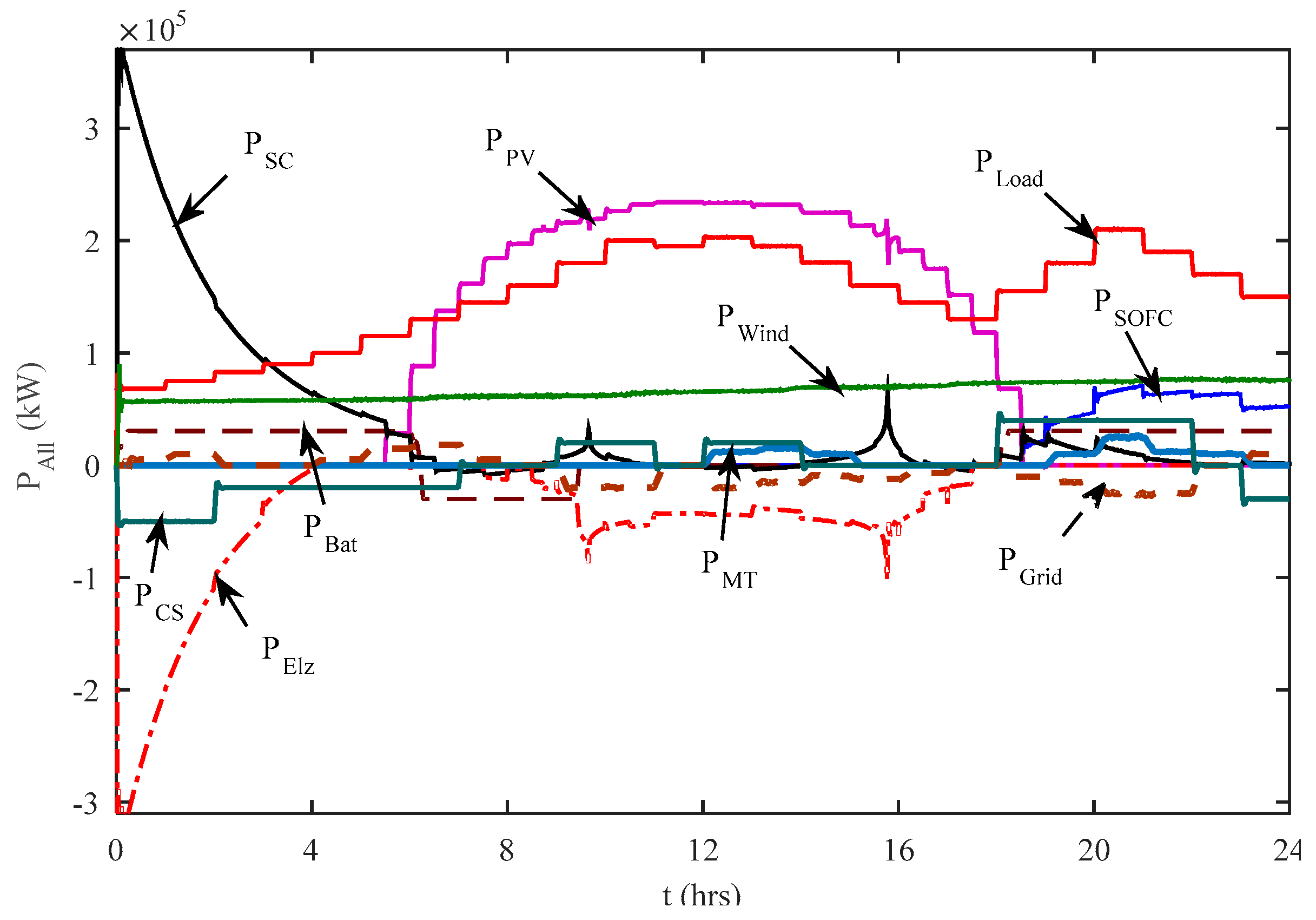
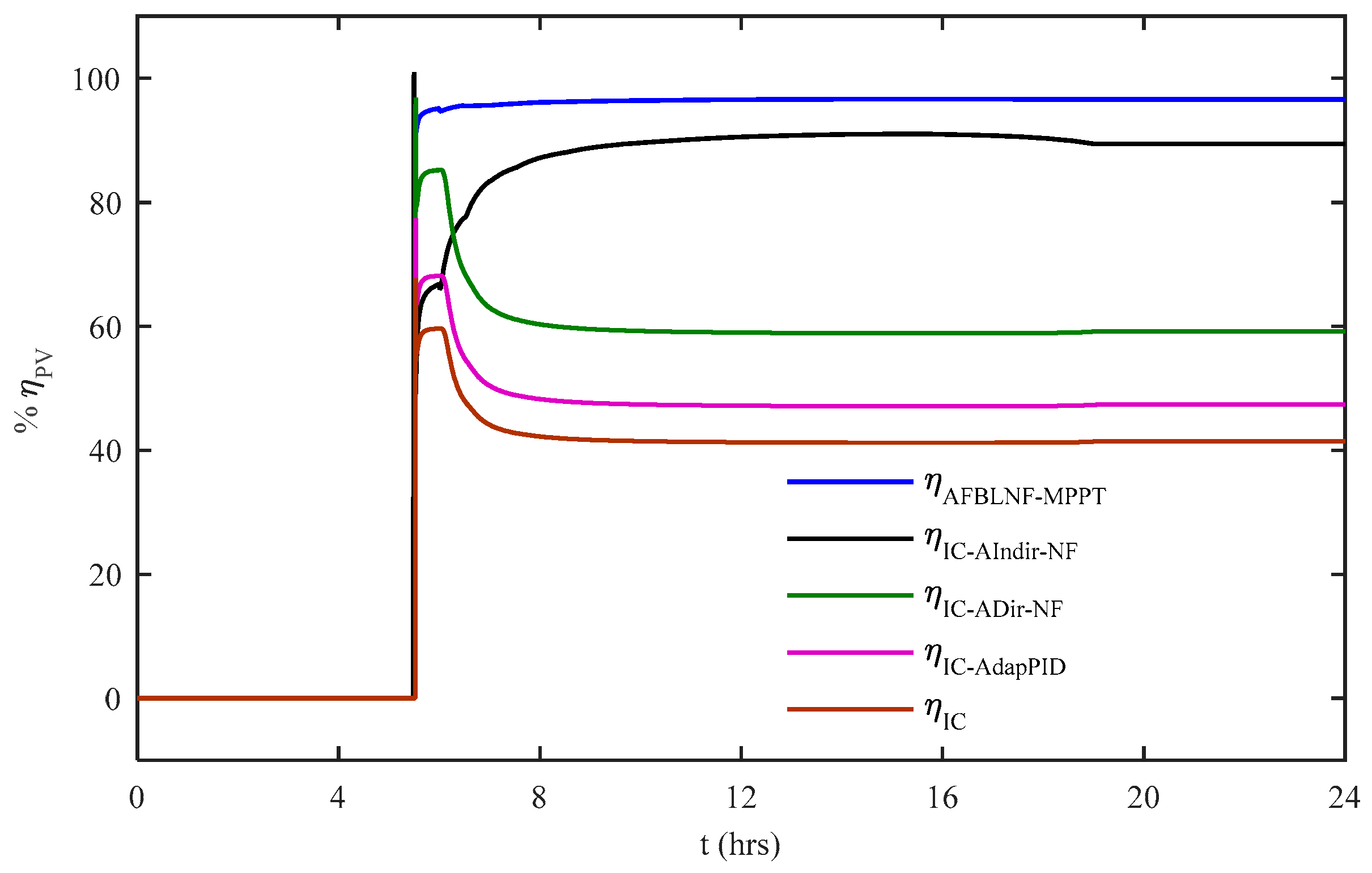
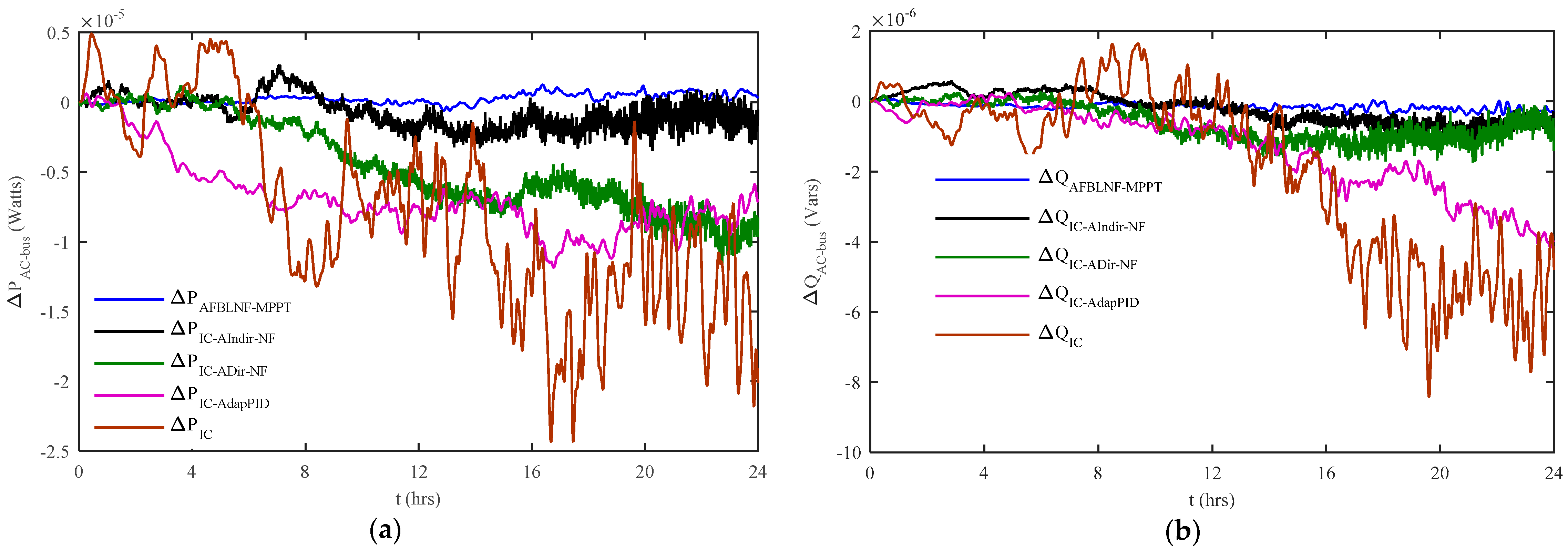
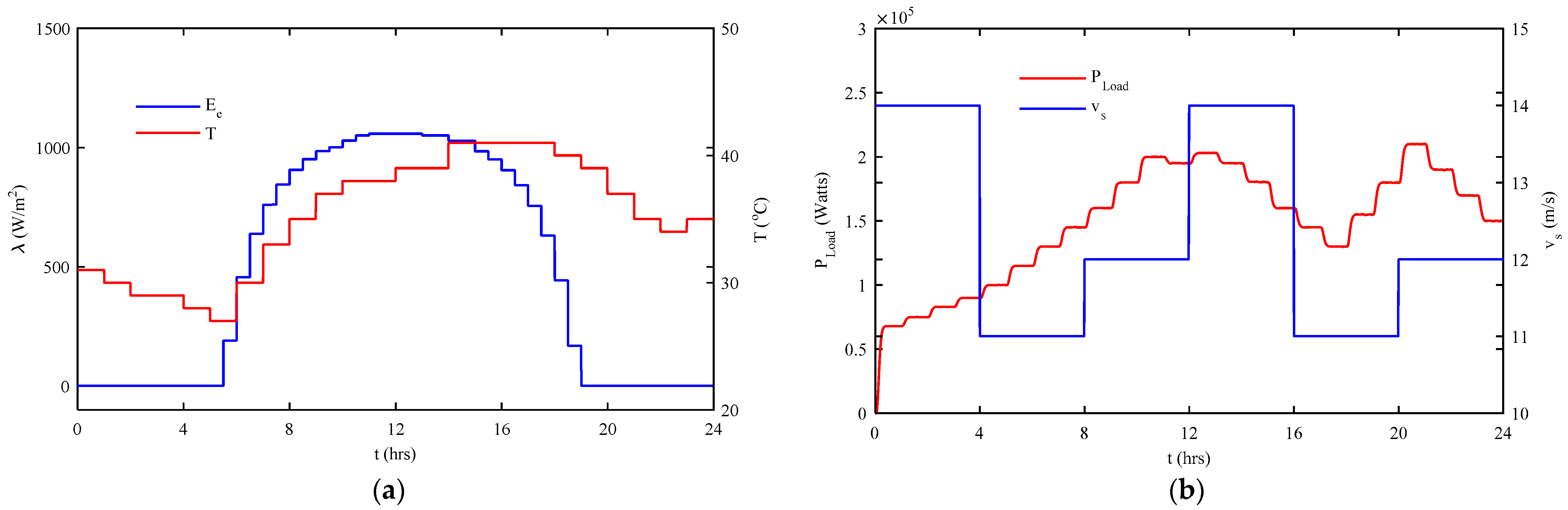
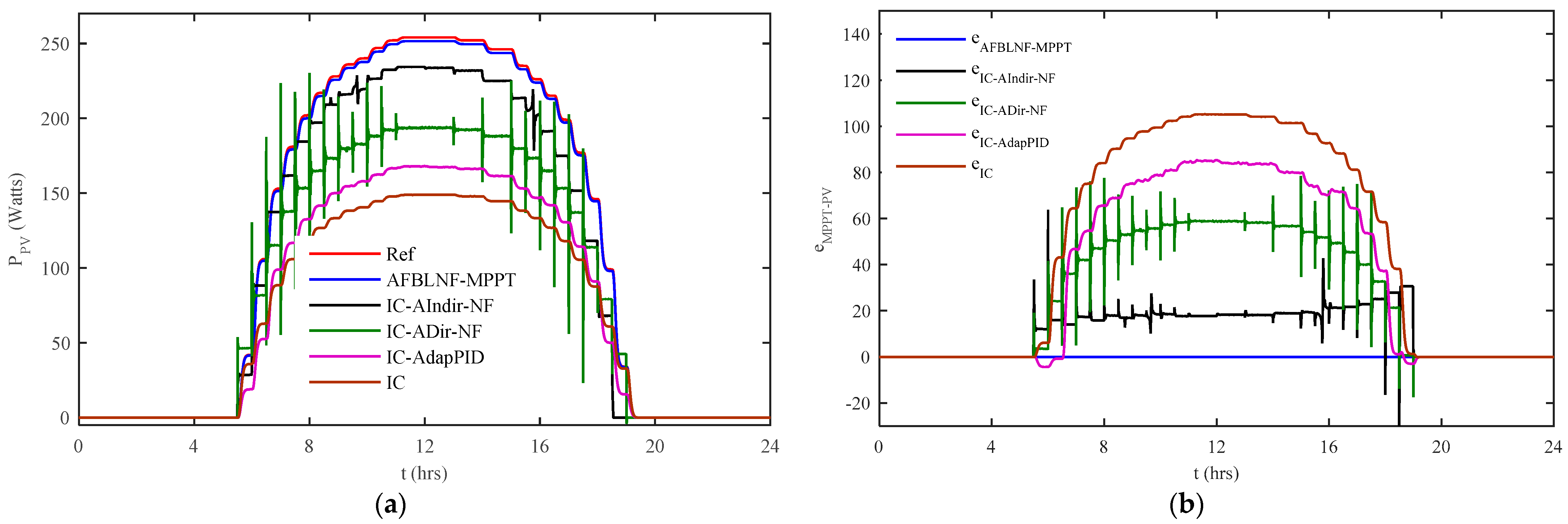
4. Results and Discussion Massachusetts

The performance of AFBLNF-MPPT for the PV subsystem is evaluated in a grid-connected HRES using MATLAB/Simulink R2015a (2015a, The MathWorks, Inc., Natick, MA, USA). The HRES consists of a UG (11 kV), wind generation (100 kW), PV (260 kW), SOFC (260 kW), an electrolyzer (150 kW), and MT (200 kVA). The battery (200 Ah) and SC (165 F) are used as backup sources. The Simulink models of WT, PV, SOFC, the electrolyzer, the battery, SC, and MT used in this work have been presented in [21]. All the sources of HRES are modeled for the cumulative dynamic load of the residential and CS. Defense Housing Authority (DHA), Islamabad, Pakistan, is considered as a case study. The irradiance (λ), ambient temperature (T), and wind speed (vs) levels are obtained from the Pakistan Meteorological Department (PMD). Figure 3 shows the irradiance, ambient temperature, wind speed, and load levels for 22 June 2015.
The irradiance for 0–5.5 h and 18.5–24 h is zero due to the absence of sun power, while a maximum of 1058 (W/m2) irradiance level is recorded during 11–13 h. Temperature varies from 27–41 °C during 0–24 h, as shown in Figure 3a. Wind speed and load power are shown in Figure 3b. Wind speed varies between 11–14 m/s. According to Figure 3b, 10–15 h and 17–22 h are the peak demand hours.
The load and generated powers of all energy sources of the HRES are shown in Figure 4. In the stated HRES, the supervisory control policy is responsible for making sure that uninterrupted and reliable power is delivered to the load [22]. According to supervisory control policy, the power acquired from wind and PV is initially utilized by the load. When renewable power is unable to meet the load, then auxiliary sources of HRES play their role correspondingly to meet the load.
The maximum pobatwers extracted by the PV subsystem using AFBLNF-MPPT, IC-AIndir-NF, IC-ADir-NF, IC-AdapPID, and IC are shown in Figure 5a. The AFBLNF-MPPT acquires the PV subsystem output power with steady state error =2.5 kW, overshoot = 0%, and undershoot = −1%. The output PV power obtained by IC-AIndir-NF has steady state error = 19.7 kW, overshoot = 15%, and undershoot = −20%. The IC-ADir-NF extracts the PV output power with steady state error = 60 kW, overshoot = 61%, and undershoot = −60%. The IC-AdapPID has steady state error = 86.5 kW, overshoot = 0%, and undershoot = −5%. The IC has steady state error = 105 kW, overshoot = 0%, and undershoot = −14%. The AFBLNF-MPPT has minimal steady state error, percent overshoot, and percent undershoot as shown in Figure 5b.
The dynamic power conversion efficiency is the ratio of PV output power to the input power, for a given time period. The dynamic efficiency of adaptive MPPT of a PV subsystem can be calculated as follows:
η 100 = t 0 t f P P V d t t 0 t f P P V r e f d t × 100 = t 0 t f ( V P V × I P V ) d t t 0 t f P P V r e f d t × 100
where η 100 is the dynamic efficiency. t 0 = 0   h and t f = 24   h are initial and final time intervals, respectively. The dynamic efficiency for MPPT of the PV subsystem with all schemes is shown in Figure 6. The dynamic efficiency of MPPT of the PV subsystem with AFBLNF-MPPT is 97%, IC-AIndir-NF is 89.44%, IC-ADir-NF is 59.24%, IC-AdapPID is 47.38%, and IC is 41.46% at t = 24 h. The dynamic efficiency based on the AFBLNF-MPPT is at the maximum during the entire simulation time. This signifies that the AFBLNF-MPPT extracts the maximum PV output power.
In order to guarantee the stability of HRES, the DC bus power deviation and AC bus power deviation should be close to zero. Figure 7 shows the DC bus power deviation with all control schemes. It is clear from the Figure 7 that the AFBLNF-MPPT has DC bus power deviation which is close to zero.
Also, the power deviations on AC bus are presented in Figure 8. The power deviations on AC bus are near to zero using AFBLNF-MPPT compared to the remaining control techniques.
The harmonics in load voltage and current arise due to switching in the converters circuit which is not synchronized with the system frequency. Harmonics dissipate the power as heat. Harmonics with higher frequencies cause the voltage flickers and fluctuations in load voltage. The PV subsystem with AFBLNF-MPPT injects a constant voltage into the inverter input, which results in low magnitude harmonics. The lowest magnitude odd harmonics are injected into the AC bus with AFBLNF-MPPT, which improves the quality of load power as shown in Figure 9. The magnitude of critical odd harmonics, i.e., 3rd, 5th, 7th, and 9th, is at the minimum with AFBLNF-MPPT. A comparison of performance improvement in reducing load voltage and current harmonics with AFBLNF-MPPT compared to IC-AIndir-NF, IC-ADir-NF, IC-AdapPID, and IC control schemes is presented in Table 1. It is obvious that the percentage reduction with the AFBLNF-MPPT technique in all the concerned odd harmonics is considerably high w.r.t all other MPPT techniques.
The percentage change in total harmonic distortions (THD) for both voltage and current is shown in Figure 10. To guarantee the HRES stability and power quality, the percentage change in voltage THD and current THD complies with the IEEE Std. 1547 [30]. The AFBLNF-MPPT controller has a flat profile compared to the other control schemes for the percentage change in voltage THD and current THD.

5. Conclusions

In this article, an AFBLNF-MPPT technique for a PV subsystem in a grid-tied HRES has been presented The results clearly show that the proposed adaptive feedback linearization-based MPPT control scheme adequately tracks the PV maximum power trajectory compared to IC-AIndir-NF, IC-ADir-NF, IC-AdapPID, and IC. The proposed control paradigm, AFBLNF-MPPT, has a higher precision than IC-AIndir-NF, IC-ADir-NF, IC-AdapPID, and IC in terms of steady-state error, overshoot, undershoot, and efficiency. The simulation results verify the superiority of the proposed control scheme.

Acknowledgments

The authors received no specific funding for this work.

Author Contributions

Sidra Mumtaz and Laiq Khan conceived and designed the experiments; Sidra Mumtaz performed the experiments; Sidra Mumtaz and Saghir Ahmad analyzed the data; Sidra Mumtaz, Saima Ali, Saghir Ahmad, Laiq Khan, Syed Zulqadar Hassan, and Tariq Kamal contributed reagents/materials/analysis tools; Sidra Mumtaz wrote the paper.

Conflicts of Interest

The authors declare no conflict of interest.

Appendix A

nLMS Algorithm

If W ^ is the estimate of W , the nLMS update law based on Equation (14) is given as follows:
ϒ ^ = W ^ e C o n t + e C o n t n 1
Updating W ^ can be written as the follows:
{ min 1 2 | W ^ ( t ) W ^ ( t 1 ) | 2 s . t . ϒ = W ^ ( t ) e C o n t + e C o n t n 1
Use the Lagrangian multiplier ƛ , the objective function becomes:
J = 1 2 | W ^ ( t ) W ^ ( t 1 ) | 2 + ( ϒ W ^ ( t ) e C o n t e C o n t n 1 )
Differentiating Equation (A2) w.r.t W ^ ( t ) and ƛ . Then equate to zero as follows:
J W ^ ( t ) = W ^ ( t ) W ^ ( t 1 ) e C o n t = 0
J = ϒ W ^ ( t ) e C o n t e C o n t n 1 = 0
Using the value of W ^ ( t ) from Equation (A3) into Equation (A4),
= 1 | e C o n t | 2 { ϒ W ^ ( t 1 ) e C o n t e C o n t n 1 }
Solving Equation (A3) for W ^ ( t ) by substituting the value of ƛ :
W ^ ( t ) = W ^ ( t 1 ) + η n L M S e C o n t | e C o n t | 2 { ϒ W ^ ( t 1 ) e C o n t e C o n t n 1 }
where 0 < η n L M S < 1 is the step size. Equation (A6) defines the nLMS algorithm. In order to avoid | e C o n t | 2 = 0 , a design parameter 0 < γ > 0.1 is introduced as follows:
W ^ ( t ) = W ^ ( t 1 ) + η n L M S e C o n t | e C o n t | 2 + γ { ϒ W ^ ( t 1 ) e C o n t e C o n t n 1 }
For the very small value of errors, Equation (A7) is further simplified as follows:
W ^ ( t ) = W ^ ( t 1 ) + η n L M S e C o n t { ϒ W ^ ( t 1 ) e C o n t e C o n t n 1 }
The above update law adapts the feedback linearization controller coefficients vectors at each iteration based on tracking error to derive the most appropriate control input over a wide range of operating conditions. The initialization step for the adaptive feedback linearization controller is given as follows:
Initialization
W ^ T = [ w 1 ,   w 2 ,   ,   w n 1 ] ,   0 < η n L M S < 1   and   0 < γ > 0.1
Do it for k > 0
e C o n t = y y r e f   and   ϒ = [ W T 1 ] e C o n t
W ^ ( t ) = W ^ ( t 1 ) + η n L M S e C o n t { ϒ W ^ ( t 1 ) e C o n t e C o n t n 1 }
where t is the number of iterations.

References

  1. Mahmud, M.A.; Pota, H.R.; Hossain, M.J.; Roy, N.K. Robust partial feedback linearizing stabilization scheme for three-phase grid-connected photovoltaic systems. IEEE J. Photovolt. 2014, 2, 423–431. [Google Scholar] [CrossRef]
  2. Sidra, M.; Khan, L. Indirect adaptive neurofuzzy Hermite wavelet based control of PV in a grid-connected hybrid power system. Turk. J. Electr. Eng. Comput. Sci. 2017, 25, 4341–4353. [Google Scholar] [CrossRef]
  3. Devi, V.K.; Premkumar, K.; Beevi, A.B.; Ramaiyer, S. A modified Perturb & Observe MPPT technique to tackle steady state and rapidly varying atmospheric conditions. Sol. Energy 2017, 157, 419–426. [Google Scholar] [CrossRef]
  4. Tey, K.S.; Mekhilef, S. Modified incremental conductance MPPT algorithm to mitigate inaccurate responses under fast-changing solar irradiation level. Sol. Energy 2014, 101, 333–342. [Google Scholar] [CrossRef]
  5. Sivakumar, P.; Kader, A.A.; Kaliavaradhan, Y.; Arutchelvi, M. Analysis and enhancement of PV efficiency with incremental conductance MPPT technique under non-linear loading conditions. Renew. Energy 2015, 81, 543–550. [Google Scholar] [CrossRef]
  6. Gokmen, N.; Karatepe, E.; Ugranli, F.; Silvestre, S. Voltage band based global MPPT controller for photovoltaic systems. Sol. Energy 2013, 98, 322–334. [Google Scholar] [CrossRef]
  7. Dousoky, G.M.; Shoyama, M. New parameter for current-sensorless MPPT in grid-connected photovoltaic VSIs. Sol. Energy 2017, 143, 113–119. [Google Scholar] [CrossRef]
  8. Giustiniani, A.; Petrone, G.; Spagnuolo, G.; Vitelli, M. Low-frequency current oscillations and maximum power point tracking in grid-connected fuel-cell-based systems. IEEE Trans. Ind. Electron. 2010, 57, 2042–2053. [Google Scholar] [CrossRef]
  9. Sun, Y.; Li, S.; Lin, B.; Fu, X.; Ramezani, M.; Jaithwa, I. Artificial Neural Network for Control and Grid Integration of Residential Solar Photovoltaic Systems. IEEE Trans. Sustain. Energy 2017, 8, 1484–1495. [Google Scholar] [CrossRef]
  10. Sundarabalan, C.K.; Selvi, K.; Kubra, K.S. Performance investigation of fuzzy logic controlled MPPT for energy efficient solar PV systems. Lect. Notes Electr. Eng. 2015, 326, 761–770. [Google Scholar] [CrossRef]
  11. Daraban, S.; Petreus, D.; Morel, C. A novel MPPT (maximum power point tracking) algorithm based on a modified genetic algorithm specialized on tracking the global maximum power point in photovoltaic systems affected by partial shading. Energy 2014, 74, 374–388. [Google Scholar] [CrossRef]
  12. Babu, T.S.; Rajasekar, N.; Sangeetha, K. Modified particle swarm optimization technique based maximum power point tracking for uniform and under partial shading condition. Appl. Soft Comput. 2015, 34, 613–624. [Google Scholar] [CrossRef]
  13. Lalili, D.; Mellit, A.; Lourci, N.; Medjahed, B.; Berkouk, E.M. Input output feedback linearization control and variable step size MPPT algorithm of a grid-connected photovoltaic inverter. Renew. Energy 2011, 36, 3282–3291. [Google Scholar] [CrossRef]
  14. Lalili, D.; Mellit, A.; Lourci, N.; Medjahed, B.; Boubakir, C. State feedback control and variable step size MPPT algorithm of the three-level grid-connected photovoltaic inverter. Sol. Energy 2013, 98, 561–571. [Google Scholar] [CrossRef]
  15. Lu, Q.; Sun, Y.; Mei, S. Nonlinear Control Systems and Power System Dynamics; Springer Science & Business Media: New York, NY, USA, 2013; Volume 10, p. 376. [Google Scholar] [CrossRef]
  16. Eriksson, R.; Soder, L. On the coordinated control of multiple HVDC links using input–output exact linearization in large power systems. Int. J. Electr. Power Energy Syst. 2012, 43, 118–125. [Google Scholar] [CrossRef]
  17. Alonge, F.; Cirrincione, M.; Pucci, M.; Sferlazza, A. Input–output feedback linearization control with on-line MRAS-based inductor resistance estimation of linear induction motors including the dynamic end effects. IEEE Trans. Ind. Appl. 2016, 52, 254–266. [Google Scholar] [CrossRef]
  18. Liutanakul, P.; Pierfederici, S.; Meibody-Tabar, F. Application of SMC with I/O feedback linearization to the control of the cascade controlled-rectifier/inverter-motor drive system with a small dc-link capacitor. IEEE Trans. Power Electr. 2008, 23, 2489–2499. [Google Scholar] [CrossRef]
  19. Korayem, M.H.; Yousefzadeh, M.; Manteghi, S. Dynamics and input–output feedback linearization control of a wheeled mobile cable-driven parallel robot. Multibody Syst. Dyn. 2017, 40, 55–73. [Google Scholar] [CrossRef]
  20. Kim, J.; Croft, E.A. Full-State Tracking Control for Flexible Joint Robots with Singular Perturbation Techniques. IEEE Trans. Control Syst. Technol. 2017, PP, 1–11. [Google Scholar] [CrossRef]
  21. Ahmad, S.; Khan, L. Performance Analysis of Conjugate Gradient Algorithms Applied to the Neuro-Fuzzy Feedback Linearization-Based Adaptive Control Paradigm for Multiple HVDC Links in AC/DC Power System. Energies 2017, 10, 819. [Google Scholar] [CrossRef]
  22. Chaouachi, A.; Kamel, R.M.; Nagasaka, K. A novel multi-model neuro-fuzzy-based MPPT for three-phase grid-connected photovoltaic system. Sol. Energy 2010, 84, 2219–2229. [Google Scholar] [CrossRef]
  23. Rezvani, A.; Gandomkar, M. Modeling and control of grid connected intelligent hybrid photovoltaic system using new hybrid fuzzy-neural method. Sol. Energy 2016, 127, 1–8. [Google Scholar] [CrossRef]
  24. Sidra, M.; Khan, L. Adaptive control paradigm for photovoltaic and solid oxide fuel cell in a grid-integrated hybrid renewable energy system. PLoS ONE 2017, 12, e0173966. [Google Scholar] [CrossRef]
  25. Sidra, M.; Khan, L.; Ahmed, S.; Bader, R. Indirect adaptive soft computing based wavelet-embedded control paradigms for WT/PV/SOFC in a grid/charging station connected hybrid power system. PLoS ONE 2017, 12, e0183750. [Google Scholar] [CrossRef]
  26. Hassan, S.Z.; Li, H.; Kamal, T.; Arifoglu, U.; Sidra, M.; Khan, K. Neuro-Fuzzy Wavelet Based Adaptive MPPT Algorithm for Photovoltaic Systems. Energies 2017, 10, 394. [Google Scholar] [CrossRef]
  27. Sidra, M.; Ali, S.; Ahmad, S.; Khan, L.; Hassan, S.Z.; Kamal, T. Energy Management and Control of Plug-In Hybrid Electric Vehicle Charging Stations in a Grid-Connected Hybrid Power System. Energies 2017, 10, 1923. [Google Scholar] [CrossRef]
  28. Pradhan, R.; Subudhi, B. Design and real-time implementation of a new auto-tuned adaptive MPPT control for a photovoltaic system. Int. J. Electr. Power 2015, 64, 792–803. [Google Scholar] [CrossRef]
  29. Ahmad, S.; Khan, L. A self-tuning NeuroFuzzy feedback linearization-based damping control strategy for multiple HVDC links. Turk. J. Electr. Eng. Comput. Sci. 2017, 25, 913–938. [Google Scholar] [CrossRef]
  30. Thomas, B.; De Blasio, R. IEEE 1547 series of standards: Interconnection issues. IEEE Trans. Power Electron. 2004, 19, 1159–1162. [Google Scholar] [CrossRef]
Figure 1. Hybrid renewable energy system.
Energies 11 00606 g001
Figure 2. Adaptive Feedback linearization based NeuroFuzzy photovoltaic (PV) maximum power point tracking (MPPT). HRES: hybrid renewable energy system.
Energies 11 00606 g002
Figure 3. (a) Irradiance and ambient temperature levels; (b) wind speed and load for 22 June 2015.
Energies 11 00606 g003
Figure 4. Load vs. generated powers of all sources. SC: super-capacitor; SOFC: solid oxide fuel cell; MT: micro-turbine; CS: charging station; Bat: battery; Elz: electrolyzer.
Energies 11 00606 g004
Figure 5. PV (a) maximum power point (MPP) power (b) MPPT error with all controllers. IC: incremental conductance; AFBLNF-MPPT: adaptive feedback linearization-based NeuroFuzzy MPPT; IC-AIndir-NF: IC based adaptive indirect NeuroFuzzy; IC-ADir-NF: IC-based adaptive direct NeuroFuzzy; IC-AdapPID: IC-based adaptive proportional-integral-derivative.
Energies 11 00606 g005
Figure 6. Dynamic efficiency for MPPT of PV subsystem.
Energies 11 00606 g006
Figure 7. DC bus power deviation.
Energies 11 00606 g007
Figure 8. AC bus (a) Active power (b) Reactive power deviations.
Energies 11 00606 g008
Figure 9. Harmonics of load (a) voltage (b) current.
Energies 11 00606 g009
Figure 10. % change in load (a) voltage total harmonic distortions (THD) (b) current THD.
Energies 11 00606 g010
Table 1. Percentage improvement in odd harmonics reduction with AFBLNF-MPPT = A as compared to IC-AIndir-NF = B, IC-ADir-NF = C, IC-AdapPID = D, and IC = E control schemes.
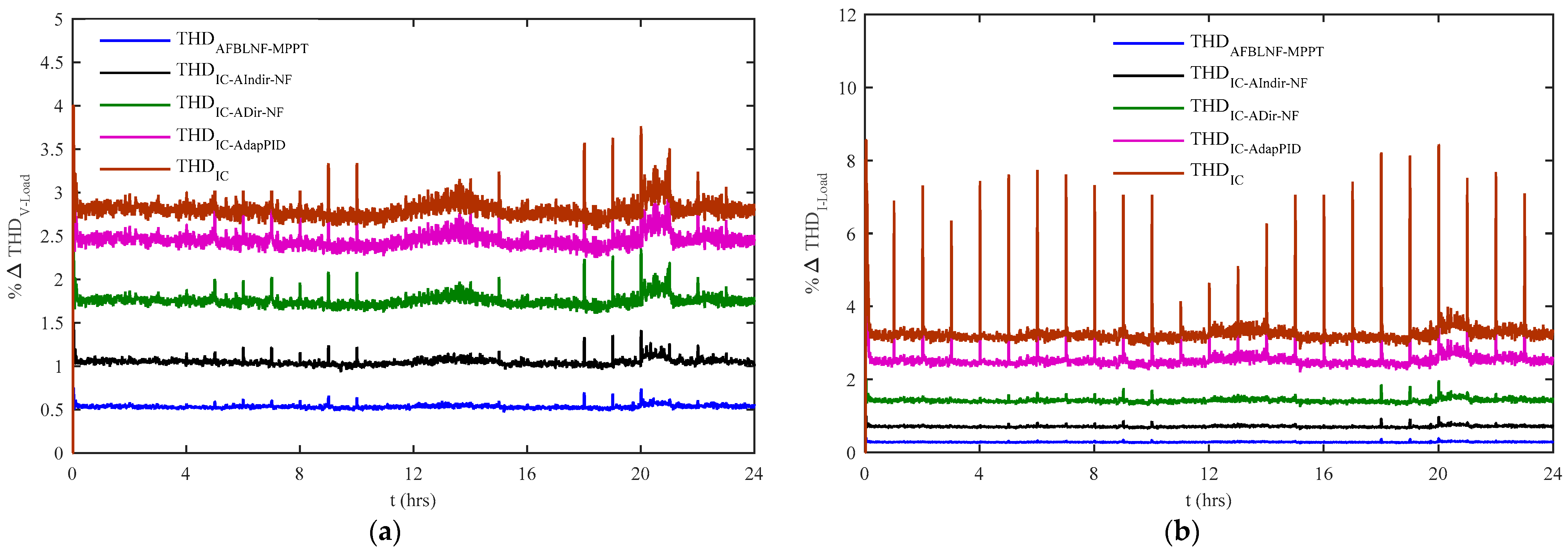
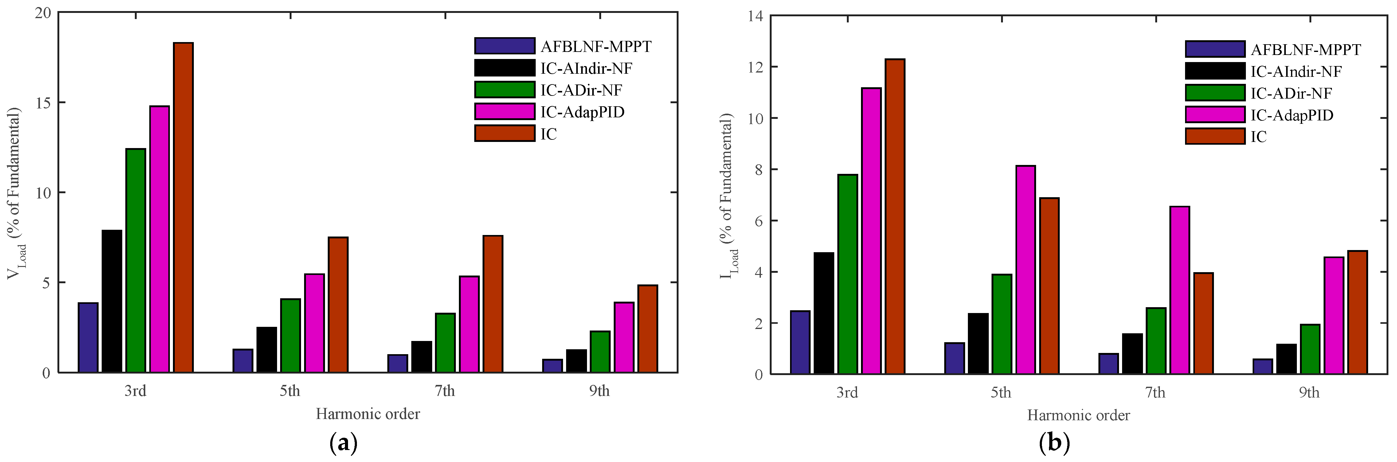
% Age Improvement in Odd Harmonics Reduction with AFBLNF-MPPT as Compared to IC-AIndir-NF, IC-ADir-NF, IC-AdapPID and IC Control Schemes
% Improvement3rd Harmonics5th Harmonics7th Harmonics9th Harmonics
VLoadILoadVLoadILoadVLoadILoadVLoadILoad
(B-A)/B %51%48%49%49%42%49%42%50%
(C-A)/C %69%68%69%69%70%69%69%70%
(D-A)/D %74%78%77%85%82%88%82%87%
(E-A)/E %79%80%83%82%87%80%85%90%

