A Fully Three Dimensional Semianalytical Model for Shale Gas Reservoirs with Hydraulic Fractures

Abstract

Two challenges exist for modeling gas transport in shale. One is the existence of complex gas transport mechanisms, and the other is the impact of hydraulic fracture networks. In this study, a truly three dimensional semianalytical model was developed for shale gas reservoirs with hydraulic fractures of various shapes. Using the instantaneous point source solution, the pressure are solved for a bounded reservoir with fully 3D, partially penetrated hydraulic fractures of different strike angles and dip angles. The fractures could have various shapes such as rectangles, disks and ellipses. The shale gas diffusion equations considers complex transport mechanism such as gas slippage and gas diffusion. This semianalytical model is verified with a commercial software and an analytical method for single fully penetrated rectangle fracture, and the production results of shale gas are consistent. The impacts of fracture height and strike angles are investigated by five systematically constructed models. The comparison shows that the production increases proportionally with the fracture height, and decreases with the increase of strike angles. The method proposed in this study could also be applied in well testing to analyze the reservoir properties and used to forecast the production for tight oil and conventional resources.

1. Introduction

Shale formations are characterized by low permeability, nanopores, high total organic carbon, and natural fractures. In shale, the gas content is mainly composed of free gas and adsorbed gas. Because of its low permeability, shale gas did not gain much success until the application of a horizontal well drilling and hydraulic fracturing technique. Currently, shale gas accounts for about half of the natural gas produced in the United States of America (U.S.A.) and that ratio will increase to 70% in 2040 according to a prediction by the U.S. Energy Information Agency [1,2] To simulate the gas production process in shales, many complex gas transport mechanisms such as gas slippage and desorption and the presence of natural fractures need to be considered, which makes the simulation of shale gas production a challenging work.

There are mainly three gas coexisting transport mechanisms during the gas production process, including gas diffusion, gas slippage and gas desorption [3]. The complexity of these mechanisms makes the classical free gas diffusivity equations inadequate to model the gas transport in shales. Despite the availability of some existing models for simulation of gas transport in shales [4,5], most of them do not fully capture the complex mechanisms, and a comprehensive gas transport equation is still needed.

Another challenge presented when dealing with shale gas transport simulation is the modeling of complex fracture patterns. The dual-porosity or dual permeability model [6,7] is widely used in numerical simulations of the fractures, but the model is usually over-simplified compared to the actual field complexities, and the resolution of this approach is not enough to capture the details of fractures. In that respect, discrete-fracture models (DFM), using finite-volume or finite-difference methods, have been developed [8]. To be compatible with the complex geometries of fractures, such as nonplanar fractures and fractures with variable aperture, reservoir simulators using unstructured grids have also been designed [9,10,11,12] in order to explicitly model the fractures. However, the use of unstructured grids leads to high computational cost so that it is only used in limited applications in real field studies. As a solution, a technique that directly incorporates complex fractures in a conventional structured grid was developed [13,14], and Moinfar et al. [15] named it embedded discrete fracture model (EDFM). The EDFM was further developed for 3D reservoir simulation by Moinfar et al. [16]. Recently, the EDFM has been widely used for naturally and hydraulically fractured reservoirs [17,18,19,20]. Despite the accurate capture of the fracture geometries, the EDFM method needs extra computation time to calculate the extra transmissibility caused by the non-neighborhood connections between fractures and matrix cells.

Assuming the rock properties are homogeneous, there are many analytical and semianalytical models derived to efficiently simulate the gas transport in shales. Gringarten et al. [21] used Green’s functions to solve unsteady flow problems for a wide variety of reservoir flow problems. Cinco-Lay and Samaniego [22] presented a new technique for analyzing pressure transient data for wells intercepted by a finite conductivity vertical fracture. Wan and Aziz [23] described a new semianalytical solution for horizontal wells with multiple fractures with different strike angles and fully/partially penetrating the formation in the vertical direction. With that solution, the authors calculated the well index combined with a numerically computed gridblock pressure. Lin and Zhu [24] studied the well performance for fractured horizontal wells in an infinite slab reservoir, by using the instantaneous solutions of plane sources. Zhou et al. [25] designed a semianalytical model to simulate the gas production in Barnett shales with fully penetrated planar fractures. Yu et al. [26] extended Zhou’s model to simulate well production for reservoirs with fully penetrated non-planar fractures, which have varying fracture width and fracture permeability. Their model was verified with a numerical reservoir simulator for single fracture case before being applied to several case studies based on Marcellus shale properties. Yang et al. [27] developed a robust and comprehensive model for real gas transport in shales with complex non-planar fracture network, with gas diffusion and gas slippage effect considered. He et al. [28] proposed a semianalytical method to diagnose the locations of underperforming fully penetrated hydraulic fractures through pressure transient analysis in tight gas reservoirs. Wang et al. [29] constructed a semianalytical model for simulating shale gas reservoirs with complex fully penetrated fractures.

In most of the above studies, due to the complexity of deriving the explicit pressure solutions for partially penetrated fractured in a bounded reservoir, the fractures are assumed to be fully penetrated rectangle shapes in a slab reservoir. Because coupling pressure and flow rate could bring an extra difficulty, most of the previous work concentrate on the pressure profile without being concerned about the production. In real situations, the fractures are most likely partially penetrated and have various shapes, such as disk and ellipse [30,31,32]. In this study, a novel semianalytical model is designed for bounded reservoir with multiple fully or partially penetrated fractures with various shapes such as rectangles, disks, and ellipses. First, the pressure solutions for fractures with dip angles or strike angles, and various shapes of fractures are derived, including rectangle, ellipse and disk shapes. Based on the pressure solutions and the mathematical equation developed for shale gas reservoirs with proper assumptions, the semianalytical model is introduced and described. The new model is verified against a commercial reservoir simulator and an analytical model for a bounded reservoir with a horizontal well and three fully penetrated fractures. In order to investigate the impact of fracture heights and strike angles on gas production, this model is then used to model the shale gas production for five bounded reservoirs with different hydraulic fracture patterns, varying from fully penetrated to partially penetrated, from fractures without strike angles to fractures with different strike angles. To the best of the authors’ knowledge, this study is the first to design a semianalytical model for shale gas reservoirs with partially penetrated fractures of various shapes. The methodology proposed in this study could be expanded and implemented in existing reservoir simulation tools to investigate various fracture patterns.

2. Materials and Methods

2.1. Model Development

For gas transport from shale matrix into fracture segment, the diffusivity equation is revised for conventional gas reservoirs by considering the important gas transport mechanisms such as gas slippage, gas diffusion, and gas desorption as follows:

$$\left[\varphi +\left(1-\varphi \right)K_a\right]c_g{\rho }_g\frac{\partial p}{\partial t}=\nabla \cdot \left\{\left(1-V_a\right)\left[\frac{{\rho }_{g}k\left(1+8\alpha K_n\right)}{{\mu }_g}+\frac{\delta }{\tau }\varphi D_g{\rho }_g{c}_g\right]\nabla p\right\}$$

(1)

where ${\rho }_g$ is gas density, $\varphi$ is rock porosity, $k$ is reservoir permeability, $C_g$ is the isothermal gas compressibility factor, $p$ is pressure, ${\mu }_g$ is gas viscosity, $V_a$ is pore volume fraction of adsorbed gas, $K_n$ is Knudsen number, $\alpha$ is a constant and close to 1, $8\alpha K_n$ is used to describe the gas slippage effect [33], $D_g$ is the Fickian diffusivity of gas component through the pore and used to describe the gas diffusion process, which might be the combination of three distinct mechanisms acting individually or simultaneously: bulk diffusion, Knudsen diffusion and surface diffusion [34]. $\delta$ is a dimensionless constrictivity factor (≤1), which accounts for variation of the pore size along its length caused by small pores and can be calculated by the empirical equation developed by Satterfield et al. [35]:

$$\delta ={\left(1-\frac{d_{\mathrm{gas}}}{d_{\mathrm{pore}}}\right)}^2$$

(2)

where $d_{\mathrm{gas}}$ is gas molecule diameter (methane molecular diameter is 0.38 nm) and $d_{\mathrm{pore}}$ is the pore diameter, $\tau$ is a dimensionless tortuosity factor (≥1), which can be estimated from porosity and gas saturation by [36]:

$$\tau =\frac{1}{{\varphi }^{1/3}{S}_g{}^{7/3}}$$

(3)

where $S_g$ is gas saturation, $K_a$ is the differential equilibrium partitioning coefficient of gas at a constant temperature, which is used to describe the gas desorption mechanism and defined as [37]:

$$K_a={\left(\frac{\partial {\rho }_a}{\partial {\rho }_g}\right)}_T$$

(4)

where ${\rho }_a$ is the adsorbed gas mass per unit shale volume (kilograms of adsorbed gas per cubic meter of solid). A general form of Brunauer–Emmett–Teller (BET) isotherm is used to model gas desorption effect [38], which is given below:

$$v(p)=\frac{v_{m}Cp/p_o}{1-p/p_o}\left[\frac{1-(n+1){\left(p/p_o\right)}^n+n{\left(p/p_o\right)}^{n+1}}{1+(C-1)p/p_o-C{\left(p/p_o\right)}^{n+1}}\right]$$

(5)

where $\nu \left(p\right)$ is the gas volume of adsorption at pressure $p$, $p_o$ is the saturation pressure of the gas, ${\nu }_m$ is the maximum adsorption gas volume when the entire adsorbent surface is being covered with a complete monomolecular layer, $C$ is a constant related to the net heat of adsorption, $n$ is number of the adsorption layers. Note that when $n=1$, Equation (5) will reduce to the standard Langmuir isotherm [39]. For the general form of BET isotherm, the differential equilibrium partitioning coefficient of gas can be expressed as:

$$K_a=\frac{{\rho }_g\left(p_{ST},T_{ST}\right){\rho }_b}{\left(1-\varphi \right)c_g{\rho }_g}\times \left(A-B+\frac{v{p}_o}{p\left(p_o-p\right)}\right)$$

(6)

$$A=\frac{v_{m}Cp}{p_o\left(p_o-p\right)}\times \frac{n\left(n+1\right){\left(p/p_o\right)}^n-n\left(n+1\right){\left(p/p_o\right)}^{n-1}}{1+\left(C-1\right)p/p_o-C{\left(p/p_o\right)}^{n+1}}$$

(7)

$$B=\frac{v}{p_o}\times \frac{C-1-C\left(n+1\right){\left(p/p_o\right)}^n}{1+\left(C-1\right)p/p_o-C{\left(p/p_o\right)}^{n+1}}$$

(8)

For gas flow from fracture to wellbore, the non-Darcy flow effect is considered by using the Forchheimer [40] modification to Darcy’s law below:

$$-\nabla p=\frac{{\mu }_g}{k}v+\beta {\rho }_g{v}^2$$

(9)

where $v$ is velocity, β is the non-Darcy Forchheimer coefficient, which can be determined using the correlation proposed by Evans and Civan [41] as given below:

$$\beta =\frac{1.485\times {10}^9}{k_f{}^{1.021}}$$

(10)

where $k_f$ is the fracture permeability.

2.2. 3D Semianalytical Methods

Using the method of images and considering the geometry, we can generate the solution for a unit-strength, instantaneous point source in an infinite-slab reservoir with impermeable boundaries at z = 0 and h, which is given below [42]:

$$\begin{array}{l}S(M,M^{\prime },t-\tau )=\frac{1}{8\sqrt{{\eta }_x{\eta }_y{\eta }_z}{[\pi (t-\tau )]}^{\raisebox{1ex}{$3$}\!\left/ \!\raisebox{-1ex}{$2$}\right.}}\exp \left[\frac{{(x-x^{\prime })}^2/{\eta }_x+{(y-y^{\prime })}^2/{\eta }_y}{4(t-\tau )}\right]\\ \cdot {\displaystyle \sum _{n=-\infty }^{+\infty }\left\{\exp \left[-\frac{{(z-z^{\prime }-2nh)}^2}{4{\eta }_z(t-\tau )}\right]+\exp \left[-\frac{{(z+z^{\prime }-2nh)}^2}{4{\eta }_z(t-\tau )}\right]\right\}}\end{array}$$

(11)

where ${\eta }_x,{\eta }_y,{\eta }_z$ is the hydraulic conductivity defined as ${\eta }_i=\frac{k_i}{\varphi \mu c_t}\left(i=x,y,z\right)$, and $M$ is the interest point and $M^{\prime }$ is the source point.

If we assume the hydraulic conductivity is isotropic, then Equation (11) could be rewritten as follows:

$$S(M,M^{\prime },t-\tau )=\frac{1}{8{[\eta \pi (t-\tau )]}^{\raisebox{1ex}{$3$}\!\left/ \!\raisebox{-1ex}{$2$}\right.}}\exp \left[\frac{{(x-x^{\prime })}^2+{(y-y^{\prime })}^2}{4\eta (t-\tau )}\right]\cdot {\displaystyle \sum _{n=-\infty }^{+\infty }\left\{\exp \left[-\frac{{(z-z^{\prime }-2nh)}^2}{4\eta (t-\tau )}\right]+\exp \left[-\frac{{(z+z^{\prime }-2nh)}^2}{4\eta (t-\tau )}\right]\right\}}$$

(12)

Using the superposition theory, we can get the pressure solution for rectangles with no strike angles (Figure 1a) as follows:

$$\begin{array}{l}p(x,y,z,t)=\frac{q_j/\rho }{8\varphi c_t{h}_f{(\pi \eta )}^{3/2}}{\displaystyle {\int }_0^t{\displaystyle {\int }_{y_1}^{y_2}\frac{1}{{\tau }^{3/2}}}}\exp \left[\frac{{(x-x_w)}^2+{(y-y^{\prime })}^2}{4\eta \tau }\right]\\ \cdot {\displaystyle {\int }_{z_w-\frac{hf}{2}}^{z_w+\frac{h_f}{2}}{\displaystyle \sum _{n=-\infty }^{+\infty }\left\{\exp \left[-\frac{{(z-z^{\prime }-2nh)}^2}{4\eta \tau }\right]+\exp \left[-\frac{{(z+z^{\prime }-2nh)}^2}{4\eta \tau }\right]\right\}}d{z}^{\prime }d{y}^{\prime }}d\tau \end{array}$$

(13)

Rewriting Equation (13) we get:

$$\begin{array}{l}p(x,y,z,t)=\frac{q_j/\rho }{8\varphi c_t{h}_f{(\pi \eta )}^{3/2}}{\displaystyle {\int }_0^t{\displaystyle {\int }_{y_1}^{y_2}\frac{1}{{\tau }^{3/2}}}}\exp \left[\frac{{(x-x_w)}^2+{(y-y^{\prime })}^2}{4\eta \tau }\right]\\ \cdot {\displaystyle {\int }_{-\frac{h_f}{2}}^{\frac{h_f}{2}}{\displaystyle \sum _{n=-\infty }^{+\infty }\left\{\begin{array}{l}\exp \left[-\frac{{((z-z_{\min })+(z_w-z^{\prime })-2nh)}^2}{4\eta \tau }\right]+\\ \exp \left[-\frac{{((z-z_{\min })+(-z_w-z^{\prime })-2nh)}^2}{4\eta \tau }\right]\end{array}\right\}}d{z}^{\prime }d{y}^{\prime }}d\tau \end{array}$$

(14)

where $x_w,y_w,z_w$ is the fracture center. Calculating the integration with respect to Z gives:

$$\begin{array}{l}{\displaystyle {\int }_{-\frac{h_f}{2}}^{\frac{h_f}{2}}{\displaystyle \sum _{n=-\infty }^{+\infty }\left\{\exp \left[-\frac{{((z-z_{\min })+(z_w-z^{\prime })-2nh)}^2}{4\eta \tau }\right]\right\}}dz=}\\ -2\sqrt{\eta \tau }\left[erf(\frac{((z-z_{\min })+(z_w-\frac{h_f}{2})-2nh)}{2\sqrt{\eta \tau }})-erf(\frac{((z-z_{\min })+(z_w+\frac{h_f}{2})-2nh)}{2\sqrt{\eta \tau }})\right]\end{array}$$

(15)

Similarly:

$$\begin{array}{l}{\displaystyle {\int }_{-\frac{h_f}{2}}^{\frac{h_f}{2}}{\displaystyle \sum _{n=-\infty }^{+\infty }\left\{\exp \left[-\frac{{((z-z_{\min })+(-z_w-z^{\prime })-2nh)}^2}{4\eta \tau }\right]\right\}}dz=}\\ -2\sqrt{\eta \tau }\left[erf(\frac{((z-z_{\min })+(-z_w-\frac{h_f}{2})-2nh)}{2\sqrt{\eta \tau }})-erf(\frac{((z-z_{\min })+(-z_w+\frac{h_f}{2})-2nh)}{2\sqrt{\eta \tau }})\right]\end{array}$$

(16)

Thus Equation (14) could be simplified to double integral expression, as follows:

$$\begin{gathered} p(x,y,z,t)=\frac{q_j/\rho }{8\varphi c_t{h}_f{(\pi \eta )}^{3/2}}{\displaystyle {\int }_0^t{\displaystyle {\int }_{y_1}^{y_2}\frac{1}{{\tau }^{3/2}}}}\exp \left[\frac{{(x-x_w)}^2+{(y-y^{\prime })}^2}{4\eta \tau }\right]\cdot \\ \left(\begin{array}{l}-2\sqrt{\eta \tau }\left[erf(\frac{((z-z_{\min })+(z_w-\frac{h_f}{2})-2nh)}{2\sqrt{\eta \tau }})-erf(\frac{((z-z_{\min })+(z_w+\frac{h_f}{2})-2nh)}{2\sqrt{\eta \tau }})\right]-\\ 2\sqrt{\eta \tau }\left[erf(\frac{((z-z_{\min })+(-z_w-\frac{h_f}{2})-2nh)}{2\sqrt{\eta \tau }})-erf(\frac{((z-z_{\min })+(-z_w+\frac{h_f}{2})-2nh)}{2\sqrt{\eta \tau }})\right]\end{array}\right)d{y}^{\prime }d\tau \end{gathered}$$

(17)

2.3. Slanted Rectangles Fracture with Strike Angle

Sometimes the fracture plane is not orthogonal to the x-y plane, but rather has a strike angle $\theta$ as plotted in Figure 1b. In this case, the pressure solution corresponding to Equation (14) will be derived as follows:

$$\begin{gathered} p(x,y,z,t)=\frac{q_j/\rho }{8\varphi c_t{h}_f{(\pi \eta )}^{3/2}}{\displaystyle {\int }_0^t{\displaystyle {\int }_{y_w-x_f\sin \theta }^{y_w+x_f\sin \theta }\frac{1}{{\tau }^{3/2}}}}\exp \left[\frac{{(x-(x_w+(y^{\prime }-y_w)\cot \theta ))}^2+{(y-y^{\prime })}^2}{4\eta \tau }\right] \\ \cdot \csc \theta \cdot {\displaystyle {\int }_{z_w-\frac{h_w}{2}}^{z_w+\frac{h_w}{2}}{\displaystyle \sum _{n=-\infty }^{+\infty }\left\{\begin{array}{l}\exp \left[-\frac{{((z-z_{\min })+(z_w-z^{\prime })-2nh)}^2}{4\eta \tau }\right]+\\ \exp \left[-\frac{{((z-z_{\min })+(-z_w-z^{\prime })-2nh)}^2}{4\eta \tau }\right]\end{array}\right\}}d{z}^{\prime }dy}d\tau \end{gathered}$$

(18)

It is necessary to point out that “$\csc \theta$” term in Equation (18) is obtained when the plane integration is performed for each fracture plane. Applying the same technique as in Equations (15) and (16), we can simplify this to the following expression:

$$\begin{gathered} p(x,y,z,t)=\frac{q_j/\rho }{8\varphi c_t{h}_f{(\pi \eta )}^{3/2}}{\displaystyle {\int }_0^t{\displaystyle {\int }_{y_w-x_f\sin \theta }^{y_w+x_f\sin \theta }\frac{1}{{\tau }^{3/2}}}}\exp \left[-\frac{{(x-(x_w+(y^{\prime }-y_w)\cot \theta ))}^2+{(y-y^{\prime })}^2}{4\eta \tau }\right]\cdot \csc \theta \\ \cdot {\displaystyle \sum _{n=-\infty }^{+\infty }2\sqrt{\eta \tau }\left\{\begin{array}{l}\left[erf(\frac{((z-z_{\min })+z_w-\frac{h_w}{2}-2nh)}{2\sqrt{\eta \tau }})-erf(\frac{((z-z_{\min })+z_w+\frac{h_w}{2}-2nh)}{2\sqrt{\eta \tau }})\right]+\\ \left[erf(\frac{((z-z_{\min })-z_w+\frac{h_w}{2}-2nh)}{2\sqrt{\eta \tau }})-erf(\frac{((z-z_{\min })-z_w-\frac{h_w}{2}-2nh)}{2\sqrt{\eta \tau }})\right]\end{array}\right\}}d{y}^{\prime }d\tau \end{gathered}$$

(19)

The corresponding bounded domain formula will become:

$$\begin{array}{l}p(x,y,z,t)=\frac{\csc \theta \cdot q_j/\rho }{8\varphi c_t{h}_f{(\pi \eta )}^{3/2}}{\displaystyle {\int }_0^t{\displaystyle {\int }_{y_w-x_f\sin \theta }^{y_w+x_f\sin \theta }\frac{1}{{\tau }^{3/2}}}}{\displaystyle \sum _{n=-\infty }^{\infty }\left\{\begin{array}{l}\exp \left[-\frac{{(x-(x_w+(y^{\prime }-y_w)\cot \theta )-2n{L}_x)}^2}{4\eta \tau }\right]+\dots \\ \exp \left[-\frac{{(x+(x_w+(y^{\prime }-y_w)\cot \theta )-2n{L}_x)}^2}{4\eta \tau }\right]\end{array}\right\}}\\ \begin{array}{l}\cdot {\displaystyle \sum _{n=-\infty }^{\infty }\left\{\exp \left[-\frac{{(y-y^{\prime }-2n{L}_y)}^2}{4\eta \tau }\right]+\exp \left[-\frac{{(y+y^{\prime }-2n{L}_y)}^2}{4\eta \tau }\right]\right\}}\\ \cdot {\displaystyle \sum _{n=-\infty }^{+\infty }2\sqrt{\eta \tau }\left\{\begin{array}{l}\left[erf(\frac{((z-z_{\min })+z_w-\frac{h_w}{2}-2nh)}{2\sqrt{\eta \tau }})-erf(\frac{((z-z_{\min })+z_w+\frac{h_w}{2}-2nh)}{2\sqrt{\eta \tau }})\right]+\\ \left[erf(\frac{((z-z_{\min })-z_w+\frac{h_w}{2}-2nh)}{2\sqrt{\eta \tau }})-erf(\frac{((z-z_{\min })-z_w-\frac{h_w}{2}-2nh)}{2\sqrt{\eta \tau }})\right]\end{array}\right\}}d{y}^{\prime }d\tau \end{array}\end{array}$$

(20)

Equation (20) will be the primary equation to be used hereafter for rectangle fractures.

2.4. Slanted Rectangles Fracture with Dip Angle

Next we study the cases in which the fracture plane is not necessarily orthogonal to the x-y plane, and instead the angle between the fracture plane and the x-y plane is set to be $\theta$.

In this case, the pressure drop solution corresponding to Equation (14) will be as follows:

$$\begin{array}{l}p(x,y,z,t)=\frac{q_j/\rho }{8\varphi c_t{h}_f{(\pi \eta )}^{3/2}}{\displaystyle {\int }_0^t{\displaystyle {\int }_{y_1}^{y_2}\frac{1}{{\tau }^{3/2}}}}\exp \left[\frac{{(x-(x_w+(z^{\prime }-z_w)\cot \theta ))}^2+{(y-y^{\prime })}^2}{4\eta \tau }\right]\cdot \csc \theta \\ \cdot {\displaystyle {\int }_{-\frac{h_w}{2}\sin \theta }^{\frac{h_w}{2}\sin \theta }{\displaystyle \sum _{n=-\infty }^{+\infty }\left\{\exp \left[-\frac{{((z-z_{\min })+(z_w-z^{\prime })-2nh)}^2}{4\eta \tau }\right]+\exp \left[-\frac{{((z-z_{\min })+(-z_w-z^{\prime })-2nh)}^2}{4\eta \tau }\right]\right\}}d{z}^{\prime }d{y}^{\prime }}d\tau \end{array}$$

which could be written as:

$$\begin{array}{l}p(x,y,z,t)=\frac{q_j/\rho }{8\varphi c_t{h}_f{(\pi \eta )}^{3/2}}{\displaystyle {\int }_0^t{\displaystyle {\int }_{y_1}^{y_2}{\displaystyle {\int }_{z_w-\frac{h_w}{2}\sin \theta }^{z_w+\frac{h_w}{2}\sin \theta }\frac{1}{{\tau }^{3/2}}\exp \left[-\frac{{(x-(x_w+(z^{\prime }-z_w)\cot \theta ))}^2+{(y-y^{\prime })}^2}{4\eta \tau }\right]}}}\\ \cdot \csc \theta \cdot {\displaystyle \sum _{n=-\infty }^{+\infty }\left\{\exp \left[-\frac{{((z-z_{\min })-z^{\prime }-2nh)}^2}{4\eta \tau }\right]+\exp \left[-\frac{{((z-z_{\min })+z^{\prime }-2nh)}^2}{4\eta \tau }\right]\right\}}d{z}^{\prime }d{y}^{\prime }d\tau \end{array}$$

(21)

If $\theta =90$, then Equation (21) will be simplified to Equation (20). The corresponding bounded domain formula will then become:

$$\begin{array}{l}p(x,y,z,t)=\frac{\csc \theta \cdot q_j/\rho }{8\varphi c_t{h}_f{(\pi \eta )}^{3/2}}{\displaystyle {\int }_0^t{\displaystyle {\int }_{y_1}^{y_2}{\displaystyle {\int }_{z_w-\frac{h_w}{2}\sin \theta }^{z_w+\frac{h_w}{2}\sin \theta }\frac{1}{{\tau }^{3/2}}}}}\\ {\displaystyle \sum _{n=-\infty }^{\infty }\left\{\begin{array}{l}\exp \left[-\frac{{(x-(x_w+(z^{\prime }-z_w)\cot \theta )-2n{L}_x)}^2}{4\eta \tau }\right]+\dots \\ \exp \left[-\frac{{(x+(x_w+(z^{\prime }-z_w)\cot \theta )-2n{L}_x)}^2}{4\eta \tau }\right]\end{array}\right\}}\\ {\displaystyle \sum _{n=-\infty }^{\infty }\left\{\exp \left[-\frac{{(y-y^{\prime }-2n{L}_y)}^2}{4\eta \tau }\right]+\exp \left[-\frac{{(y+y^{\prime }-2n{L}_y)}^2}{4\eta \tau }\right]\right\}}\\ \cdot {\displaystyle \sum _{n=-\infty }^{+\infty }\left\{\exp \left[-\frac{{((z-z_{\min })-z^{\prime }-2nh)}^2}{4\eta \tau }\right]+\exp \left[-\frac{{((z-z_{\min })+z^{\prime }-2nh)}^2}{4\eta \tau }\right]\right\}}dz\prime dy\prime d\tau \end{array}$$

(22)

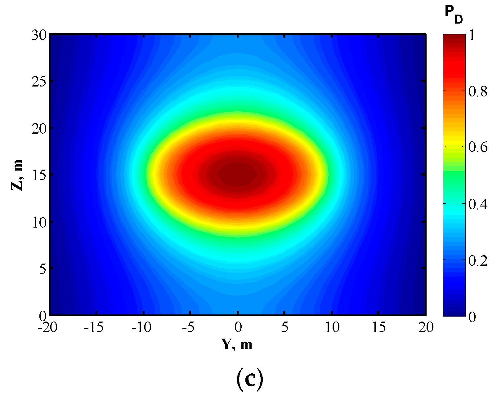
2.5. Pressure Solutions for Rectangle, Ellipse, and Disk Fractures

To show the versatility of our method, and for the purpose of faster computation, the pressure solutions for three other shapes of fractures are constructed in a slab reservoir. Following the same logic as for the rectangle fracture in a bounded reservoir, the pressure solution of other shapes could also be derived. The pressure solution for a disk fracture in a slab reservoir is given as below:

$$\begin{array}{l}p(x,y,z,t)=\frac{q_j/\rho }{8\varphi c_t{r}_w{(\pi \eta )}^{3/2}}{\displaystyle {\int }_0^t{\displaystyle {\int }_0^{2\pi }{\displaystyle {\int }_0^{r_w}\frac{1}{{\tau }^{3/2}}\exp \left[\frac{{(x-x_w)}^2+{(y-(r_w+r\cos \alpha ))}^2}{4\eta \tau }\right]}}}\\ \cdot {\displaystyle \sum _{n=-\infty }^{+\infty }\left\{\exp \left[-\frac{{((z-z_{\min })+(z_w-r\sin \alpha )-2nh)}^2}{4\eta \tau }\right]+\exp \left[-\frac{{((z-z_{\min })+(-z_w-r\sin \alpha )-2nh)}^2}{4\eta \tau }\right]\right\}}drd\alpha d\tau \end{array}$$

(23)

Similarly, the pressure solution for an ellipse fracture in a slab reservoir is given as:

$$\begin{array}{l}p(x,y,z,t)=\frac{q_j/\rho }{8\varphi c_t{r}_w{(\pi \eta )}^{3/2}}{\displaystyle {\int }_0^t{\displaystyle {\int }_0^{2\pi }{\displaystyle {\int }_0^1\frac{1}{{\tau }^{3/2}}\exp \left[\frac{{(x-x_w)}^2+{(y-(y_w+ar\cos \alpha ))}^2}{4\eta \tau }\right]}}}\cdot r\\ \cdot {\displaystyle \sum _{n=-\infty }^{+\infty }\left\{\exp \left[-\frac{{((z-z_{\min })+(z_w+br\sin \alpha )-2nh)}^2}{4\eta \tau }\right]+\exp \left[-\frac{{((z-z_{\min })+(-z_w-br\sin \alpha )-2nh)}^2}{4\eta \tau }\right]\right\}}drd\alpha d\tau \end{array}$$

(24)

Three cases are designed with three different shapes of fractures. In all three cases, the depth of the slab reservoir is 30 m, and the center of all three fractures is at (0, 15). The dimensionless pressure results after 1000 days are plotted in Figure 2. The dimensionless pressure is defined as the actual minimum and maximum pressure being translated to [0, 1] range by the linear translation. Figure 2a is a fracture with rectangular shape, where the length of the rectangle equals 20 m and the height equals 10 m. Figure 2b has a disk fracture, with radius equal to 10 m. Figure 2c has an elliptical fracture, with a long radius equal to 10 m and short radius equal to 5 m. Using Equation (17) and Equations (23) and (24), the pressure solution could be calculated. To concentrate on different pressure distribution contours caused by different shapes of the fractures, only the dimensionless pressure values are plotted. The dimensionless pressure solutions are shown in Figure 2.

Comparing Figure 2a–c, there are two observations to make. First, it shows that our pressure solutions capture the pressure contours accurately, with the boundary effect clearly seen from the top and bottom of the reservoir. Second, the fracture shape impact the pressure distribution thus the shale gas production significantly, so that it is worthwhile obtaining better measurement about the fracture shapes.

2.6. Semianalytical Model for 3D Fractures in Shale Gas Reservoir

For the non-planar fracture geometry with varying fracture width and fracture permeability along fracture length, a semi-analytical model is developed to efficiently simulate the shale gas production. The semi-analytical model discretizes the non-planar fracture geometry into a number of small fracture segments in order to approximately describe the non-planar fracture geometry. Each fracture segment can have different fracture properties such as fracture length, width, and permeability to approximately represent the non-planar fracture geometry. The semi-analytical model mainly consists of two parts for simulating shale gas production: gas flow from shale matrix into fracture and gas flow from fracture to wellbore. First, we used an analytical solution to approximately solve the revised diffusivity equation for gas transport from shale matrix into fracture segments. Second, gas flow in each fracture segment is described by the non-Darcy flow equation. For the first part, an analytical solution is used to solve the gas diffusivity equation with the following assumptions:

(1)

The reservoir is bounded;

(2)

The reservoir is isotropic and homogeneous;

(3)

It only allows gas flow from fractures to wellbore;

(4)

There is no gravity effect.

According to the superposition principle, one can calculate the pressure change at any location in the system by adding the contributions from all fracture segments. The pressure solution p_jc at the center of the j-th fracture segment $x_{jc},y_{jc},z_{jc}$ for fluid flow in shale with the following expressions:

$$p_{jc}(x_{jc},y_{jc},z_{jc},t)={\displaystyle \sum _{j=1}^{N_f}{p}_j(x_{jc},y_{jc},z_{jc},t)}$$

(25)

where $p_j\left(x_{jc},y_{jc},z_{jc},t\right)$ is defined as Equation (20) and:

$$x_{jc}=\frac{1}{2}\left(x_j+x_{j+1}\right)$$

(26)

$$y_{jc}=\frac{1}{2}\left(y_j+y_{j+1}\right)$$

(27)

$$z_{jc}=\frac{1}{2}\left(z_j+z_{j+1}\right)$$

(28)

In all cases of this study, the constant pressure well condition is assumed. In this case, the semianalytical model will discretize a fracture into N_f fracture segments with N_v nodes ($N_{\nu }=N_f+1$). All unknown that need to be solved include:

(1)

$N_f$ gas flux at fracture segments, $q_{fi}=\left(i=1,2,\cdots ,N_f\right)$.

(2)

$N_{\nu }$ gas flow rates at all nodes $q_i\left(i=1,2.\cdots N_{\nu }\right)$.

(3)

$N_{\nu }$ pressure at all nodes $p_i\left(i=1,2.\cdots N_{\nu }\right)$, but the pressure at the well node is known, so that there are $N_f$ pressure unknowns at nodes.

So there are $2N_f+N_{\nu }$ unknown variables. The corresponding equations needed to solve include:

(1)

$N_{\nu }$ mass balance equations at all nodes:

$${(q_i)}_{in\_flow}={(q_i)}_{out\_flow}$$

(29)

(2)

$N_f$ non-Darcy flow equations at all fracture segments, which are described by Equation (9).

(3)

$N_f$ pressure continuity equations of all fracture segments by equating Equations (9) and (25).

Totally there are $2N_f+N_{\nu }$ equations, equal to the number of unknowns. Thus the model is well-defined. The Newton-Raphson iterative method was used to solve the final nonlinear system of governing equations, caused by the non-Darcy effect of gas flow. In the simulation, it is assumed that there is only gas flow under the condition of residual water saturation and the reservoir is homogeneous with a constant height, porosity, and permeability. It should be noted that the current semi-analytical model did not capture the effect of pressure-dependent matrix permeability with reservoir depletion. In order to analyze this effect, numerical reservoir simulation is recommended.

3. Results

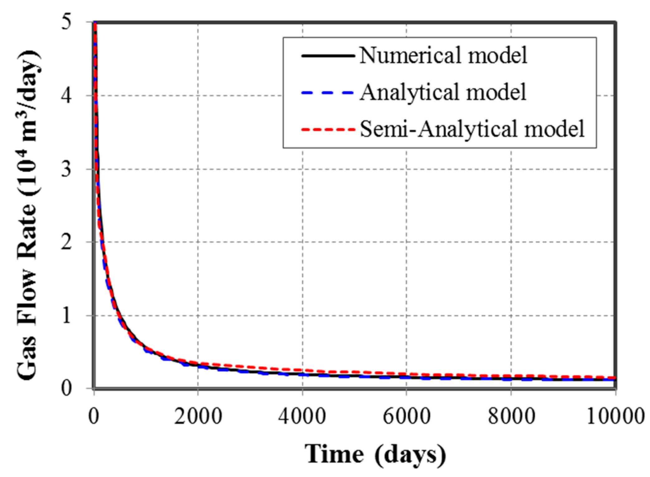
3.1. Model Validation

Before the newly derived 3D semianalytical model is used to investigate the effects of fracture height and fracture strike angles, a commercial simulator and an analytical model are used to verify the accuracy of this model. The verification case has three bi-wing hydraulic fractures and each fracture is discretized equally into 10 segments. The model dimension is 260 m × 600 m × 50 m, which corresponds to the reservoir length, width and thickness, respectively. The bottomhole pressure is held at 7.5 MPa for all simulations. Other basic reservoir, fluid and fracture parameters are listed in

Table 1. Basic parameters used for the reservoir model.

Parameter	Symbol	SI Unit	Value
Reservoir temperature	$T$	K	353.15
Initial reservoir pressure	$p_i$	MPa	38
Initial reservoir permeability	$k_i$	nD	100
Reservoir thickness	$h$	m	50
Reservoir porosity	$\varphi$	-	4%
Initial gas saturation	$S_g$	-	100%
Specific gas gravity	-	-	0.5432
Molar mass of methane	$M$	kg/mol	0.016
Diameter of methane molecule	$d$	nm	0.41
Universal gas constant	$R$	J/mol/K	8.3145
Critical pressure of methane	$p_c$	MPa	4.64
Langmuir pressure	$p_L$	MPa	6
Langmuir volume	$v_L$	m3/ton	2.5
Bulk density of shale	${\rho }_b$	kg/m3	2.6 × 103
Fracture half-length	$x_f$	m	150
Fracture height	$h_f$	m	50
Fracture spacing	-	m	30
Fracture conductivity	FC	m2∙m	3.048 × 10−14
Fracture width	$w_f$	m	0.003

.

The simulation was run for 10,000 days, for the newly developed 3D semianalytical model, an analytical model (Kappa Topaz) and a commercial reservoir simulator (CMG). The comparison results of the gas flow rates are plotted in Figure 3. The three curves in Figure 3 are so close to each other, with relative error less than 3%, illustrating that the newly developed 3D semianalytical model can accurately calculate the shale gas production for reservoirs with fully penetrated fractures. For the detailed description of the comparison, readers could refer to the authors’ another work [29].

3.2. Model Applications

After the accuracy and effectiveness of the 3D semianalytical model are verified, five cases of shale gas reservoirs with different fracture patterns are constructed, in order to study the impact of fracture height and strike angles on shale gas production. In general, the gas production is controlled by many properties of the fracture and matrix, such as permeability, fracture conductivity, but to focus on the major innovations of this study, which is the construction of a truly three dimensional hydraulic fracture model, with different strike/dip angles, we only analyze the impacts of fracture heights and strike angles. The five cases are summarized as follows:

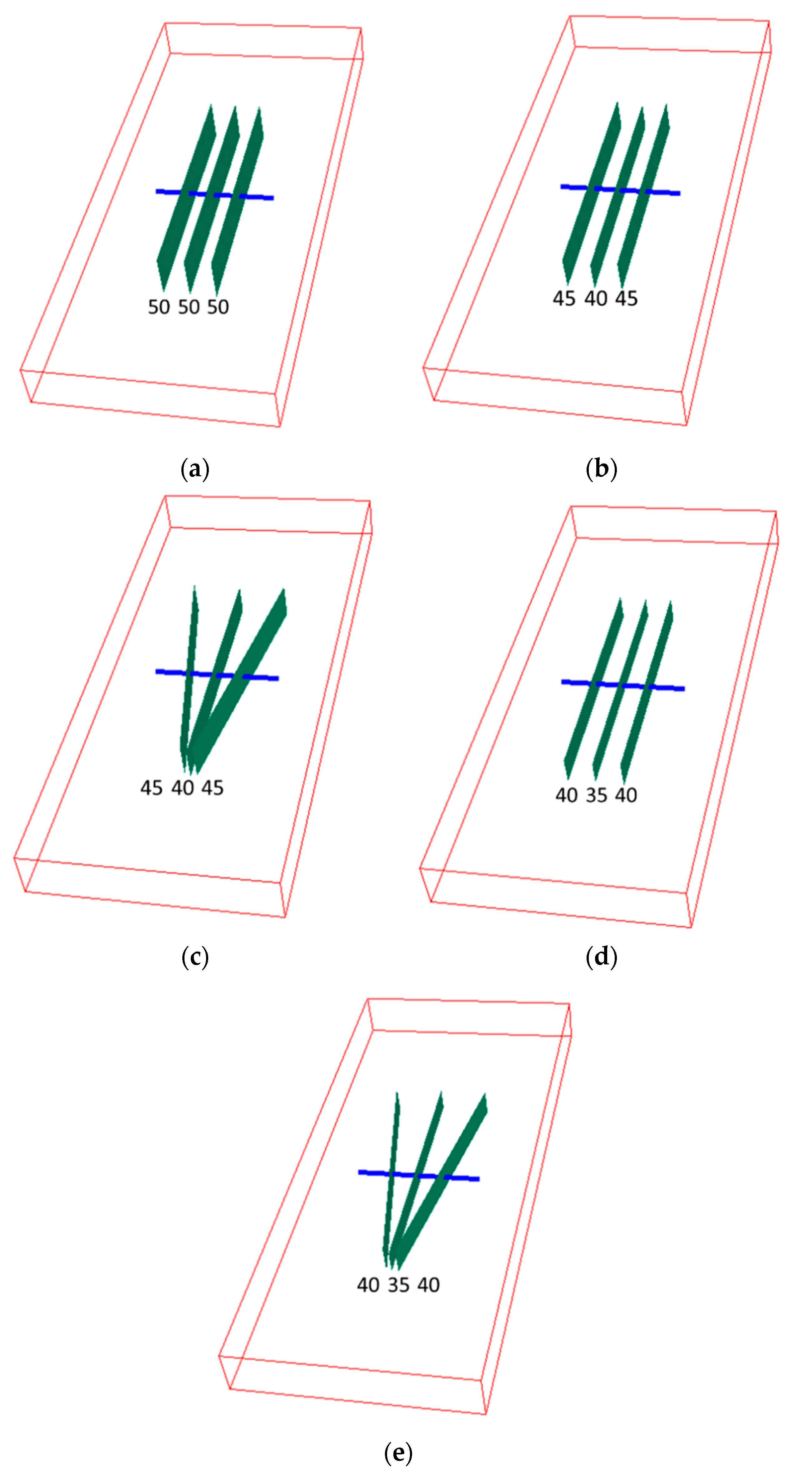
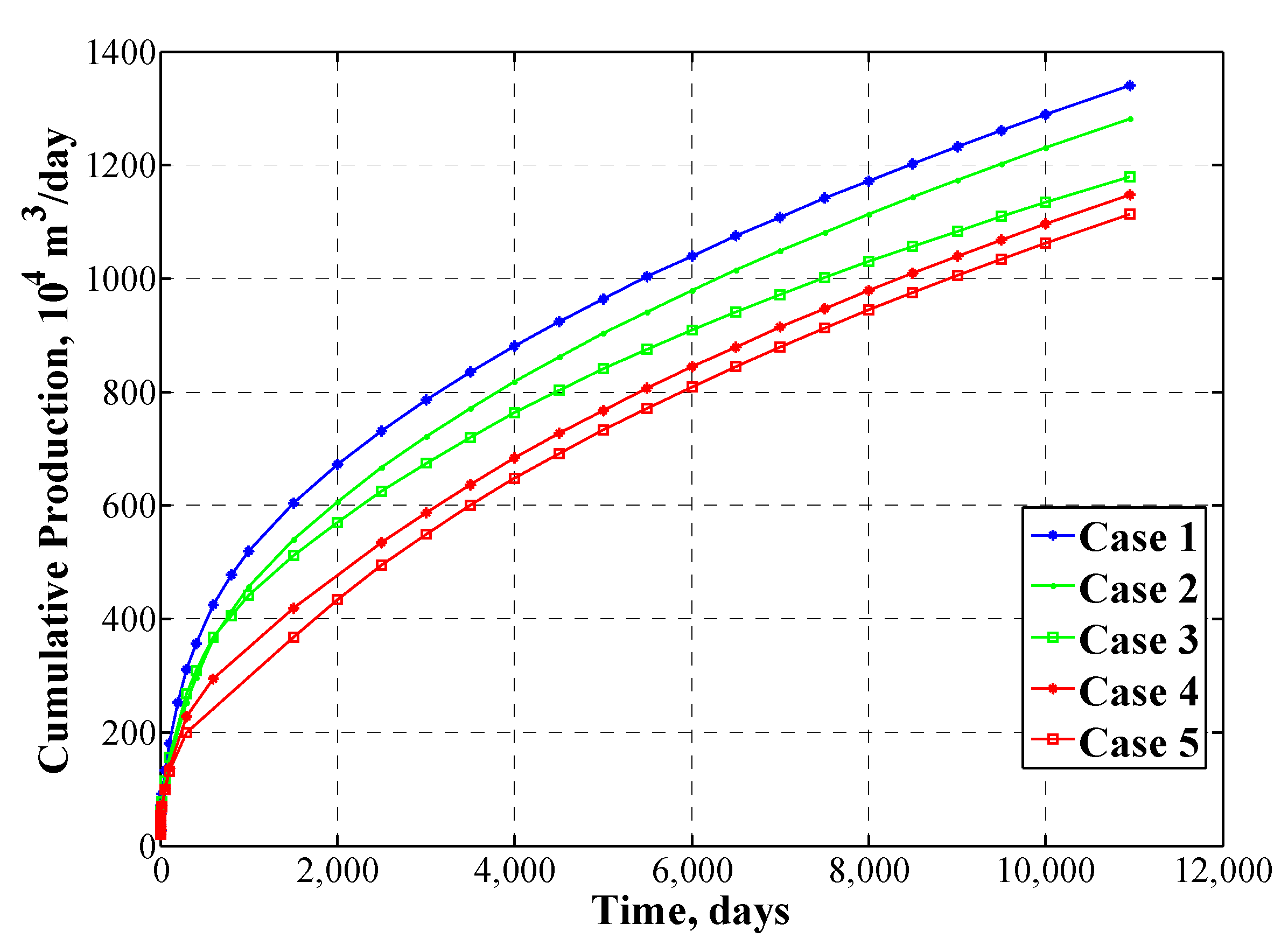
• Case 1: Three fully penetrated fractures, with fracture heights 50 m, 50 m and 50 m, and strike angles 0°, 0°and 0°.
• Case 2: Three partially penetrated fractures, with fracture heights are 45 m, 40 m, and 45 m, and strike angles 0°, 0°and 0°.
• Case 3: Three partially penetrated fractures, with fracture heights are 45 m, 40 m, and 45 m, and strike angles −10°, 0°and 10°.
• Case 4: Three partially penetrated fractures, with fracture heights are 40 m, 35 m, and 40 m, and strike angles 0°, 0°and 0°.
• Case 5: Three partially penetrated fractures, with fracture heights are 40 m, 35 m, and 40 m, and strike angles −10°, 0°and 10°.

The fracture patterns of these five cases and the corresponding reservoir models are plotted in Figure 4. The green planes are the fractures, with different strike angles and fracture heights. The blue lines are the horizontal wells. The reservoir size and well properties are the same for all five cases, but the fracture heights and strike angles are different.

The differences between Case 1, Case 2/3 and Case 4/5 are the fracture heights. Case 1 (Figure 4a) has three hydraulic fractures with 50 m height, which are fully penetrated in the reservoir. Cases 2 and 3 (Figure 4b, c) have three fractures with variant heights, 45 m, 40 m and 45 m from left to right. Case 4 and Case 5 (Figure 4d and Figure 2e) have three fracture with heights 40 m, 35 m and 40 m. The differences between Case 2 and Case 3 are the strike angles. Case 2 has three fractures with 0° strike angles, but Case 3 has tree fractures with strike angles −10°, 0°and 10°. The same strike angle difference exists for Case 4 (Figure 4d) and Case 5 (Figure 4e).

The model dimensions (length, width and thickness) for the five cases are the same: 260 m × 600 m × 50 m. The bottomhole pressure is held at 7.5 MPa for all simulations. Other basic reservoir, fluid and fracture parameters are still the same with Table 1. Using the semianalytical model we just developed and verified, the gas production of five cases are computed.

First, by just analyzing Case 2, the impact of fracture height could be investigated. Figure 5 shows the production data for each fracture in Case 2. To show the difference, the semi-log plot on y axis is used. The blue line is the daily production rate of the first and third fractures with 45 m height, and the red line is for the second fracture with 40 m height. It is clear that the higher fractures have more shale gas produced than the lower one. In fact, at the early stage (from day 1 to day 50), the increase of production for higher fracture is about 12.5%. But in late stage (after 4000 days), that increment could become 400%. The production data of single fractures for other cases have similar comparison results (15% and 500%).

To investigate the impact of fracture height and strike angles, we compare the cumulative production data for these five cases, which are plotted in Figure 6, which shows that the cumulative production data for these five cases are decreasing as the fracture heights decrease and the strike angle variates. In fact, after 2500 days, the decreasing production caused by fracture height between Case 1 and Case 2 is around 10% to 15%. The corresponding ratio from Case 2 to Case 4 is about 10–20%. The decrease ratio caused by strike angles change is approximately 6–8% between Case 2 and Case 3, while the corresponding decrease ratio between Case 4 and Case 5 is approximately 3% to 8%.

Figure 6 shows clearly that the impacts of fracture areas for the shale gas productions. With decreasing fracture heights from Case 1 to Case 2 and Case 4, while their lengths are the same, the fracture areas are correspondingly decreasing. It is seen from Figure 6 that the cumulative productions of Case 1, Case 2 and Case 4 are decreasing too, with the similar ratio as the fracture heights. For example, the total fracture heights of Case 1 and Case 2 are 150 m and 130 m, respectively, and the ratio of the total heights are 87%, which is very close to the cumulative production ratio of Case 1 and Case 2. The same comparison result holds true for Case 4.

The well interference effect has also been widely studied recently [43,44,45]. In Figure 6, comparing Case 2 and Case 3, the only difference is that Case 3 has nonzero strike angles. The difference between their cumulative productions is very clear. The cumulative production of Case 3 is about 7% less than Case 4. This quantitatively verifies the impact of strike angles on shale gas production, which provides measurement criteria for fracturing design and evaluations.

4. Discussion

Shale gas production has become an important part of the energy supply of the world, especially for the United States. It will become even more dominant in the next 20 years, but modelling shale gas reservoirs production has proved challenging due to the complex fluid flow mechanisms and the existence of various fracture patterns. Although many techniques have been proposed, such as numerical methods (Finite Volume Method, Finite Element Method) based on structured or unstructured grids, analytical methods, and decline curve analysis, there is still a need to design a method that honors the complex fracture geometry while having faster computation speed. In this study, a new truly 3D semianalytical model for bounded shale gas reservoirs with various fracture patterns is designed and validated with a commercial simulator and an analytical model. Then this model is applied to investigate the impacts of fracture heights and strike angles on daily production rate and cumulative production.

To the best of the authors’ knowledge, this study is the first to rigorously derive the pressure solution for three dimensional fracture plane in a bounded shale gas reservoir. The fractures could be fully penetrated or partially penetrated. They can also have any strike angle or dip angle. The shapes are not constrained either. The pressure solutions for fractures with shapes of rectangles, disks, and ellipses have been derived explicitly. The same derivation technique could be adopted to derive pressure solutions for any shape of fractures with explicit expressions of the planes.

For complicate shapes of fractures such as disks and ellipses, the pressure solutions have the form of triple integrals. The computation of these triple integrals will be time-consuming because of the singularity existing at the end points of integral interval. In order to efficiently model shale gas reservoirs with complex fracture shapes and patterns, a better numerical integration algorithm needs to be developed and implemented into the current semianalytical model.

This study concentrates on single phase, shale gas reservoirs, but the technique proposed here could be easily expanded to simulate multiphase reservoirs. For multiphase reservoirs with fully penetrated, rectangle shape fractures, several researchers have made great effort to develop semianalytical models to model the pressure profile and production [46]. The pressure solution derived in this study could be directly implemented into multiphase semianalytical model to model more complex fluid physics.

Finally, the fractures in this study are all synthetic with uniform fracture widths, permeability, and fracture conductivity, in the purpose of concentrating on investigating the impact of fracture heights and angles systematically and quantitatively. In the future, more practical fracture patterns will be implemented into the semianalytical model by integrating seismic data or well logging data. The fracture patterns could be generated based on microseismic data and fracture outcrop figures [47,48], which will make the semianalytical model more realistic. The fracture widths, fracture conductivity could also be variables as what the authors have done before for fully penetrated nonplanar fractures [26]. The classical gas transport equations used in this study could also be replaced with fractional gas diffusion equations to include the historical dependence effect of the shales [49,50,51,52,53].

5. Conclusions

With the rapidly growing interest in unconventional resources such as shale gas, studying the impact of hydraulic fractures on shale gas production has become an urgent task for petroleum engineers. In this study, based on the gas transport equation considering multiple fluid mechanisms such as gas desorption, gas diffusion and gas slippage, a semianalytical model was constructed and solved for shale gas reservoirs with fully 3D hydraulic fractures. This method could model hydraulic fractures with different strike/dip angles and different shapes. This semianalytical model was verified with a commercial software and an analytical method. The shale gas production of reservoirs with different fracture heights and strike angles are simulated and compared. Based on our study, the following conclusions could be drawn:

• The pressure for partially penetrated fractures with different strike angles, dip angles and shapes could be derived by integrating the instantaneous point source solution on the fracture plane;
• Based on comprehensive shale gas transport equations considering complex gas transport mechanisms and complex fracture patterns, a novel semianalytical model to simulate the gas transport and production is developed by discretizing each fracture to multiple segments;
• This semianalytical mode has been verified with a commercial simulator and an analytical model for a shale gas reservoir with three fully penetrated fractures, and the relative error is within 3%;
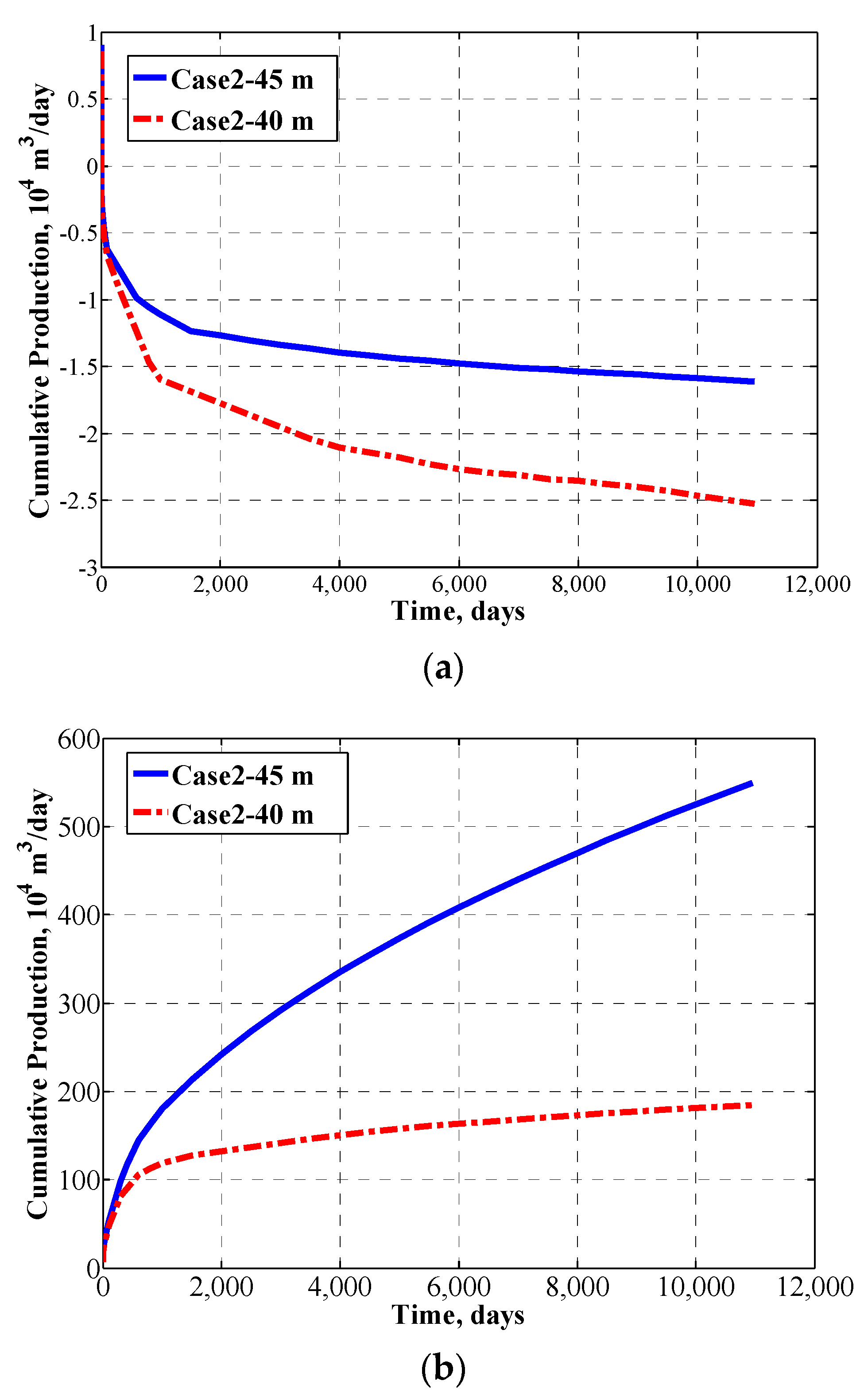
• Five shale gas reservoir cases with different fracture heights and strike angles have been investigated by using this semianalytical model. It is found that the decreasing of fracture height will lead to decreasing production rate and cumulative shale gas production, by a ratio close to the fracture areas ratio; and strike angles could cause well interference and decrease the daily production rate and cumulative shale gas production.
• The technique proposed in this study and the partial results shed a light on the importance of fracture shapes and heights. In most of the shale gas models, the hydraulic fractures are always assumed to be rectangle and fully penetrated in the pay zone. But from the results of this study, the fracture shapes and heights play essential roles in influencing the shale gas production. On the other hand, these explicit pressure results derived in this study for fracture planes with different shapes and angles could also be used in well testing to investigate the fracture and reservoir properties. Thirdly, although the cases studied here are all synthetic and simple, the methods could still be used for complex fracture patterns with the help of more accurate geophysical measurement. In conclusion, the method proposed in this work will be widely used by petroleum engineers dealing with unconventional reservoirs with complex fractures.

References

1. Energy Information Administration (EIA). Shale Gas Production Drives World Natural Gas Production Growth. 2016. Available online: http://www.eia.gov/todayinenergy/detail.cfm?id527512 (accessed on 20 December 2017).
2. Energy Information Administration (EIA). Annual Energy Outlook. 2017. Available online: https://www.eia.gov/outlooks/aeo/pdf/0383(2017).pdf (accessed on 10 December 2017).
3. Wu, K.; Li, X.; Wang, C.; Yu, W.; Chen, Z. Model for surface diffusion of adsorbed gas in nanopores of shale gas reservoirs. Ind. Eng. Chem. Res. 2015, 54, 3225–3236. [Google Scholar] [CrossRef]
4. Wang, K.; Liu, H.; Luo, J.; Wu, K.; Chen, Z. A comprehensive model coupling embedded discrete fractures, multiple interacting continua, and geomechanics in shale gas reservoirs with multiscale fractures. Energy Fuel 2017, 31, 7758–7776. [Google Scholar] [CrossRef]
5. Wu, K.; Chen, Z.; Li, J.; Li, X.; Xu, J.; Dong, X. Wettability effect on nanoconfined water flow. Proc. Natl. Acad. Sci. USA 2017, 114, 3358–3363. [Google Scholar] [CrossRef] [PubMed]
6. Warren, J.E.; Root, P.J. The Behavior of Naturally Fractured Reservoirs. Soc. Pet. Eng. J. 1963, 3, 245–255. [Google Scholar] [CrossRef]
7. Kazemi, H.; Gilman, J.R.; Eisharkawy, A.M. Analytical and numerical solution of oil recovery from fractured reservoirs with empirical transfer functions. SPE Reserv. Eng. 1992, 7, 219–227. [Google Scholar] [CrossRef]
8. Zhang, Y.; Gong, B.; Li, J.; Li, H. Discrete Fracture Modeling of 3D Heterogeneous Enhanced Coalbed Methane Recovery with Prismatic Meshing. Energies 2015, 8, 6153–6176. [Google Scholar] [CrossRef]
9. Noorishad, J.; Mehran, M. An upstream finite element method for solution of transient transport equation in fractured porous media. Water Resour. Res. 1982, 18, 588–596. [Google Scholar] [CrossRef]
10. Matthäi, S.K.; Mezentsev, A.; Belayneh, M. Control-Volume Finite-Element Two-Phase Flow Experiments with Fractured Rock Represented by Unstructured 3D Hybrid Meshes. In Proceedings of the SPE Reservoir Simulation Symposium, The Woodlands, TX, USA, 31 January–2 February 2005; Society of Petroleum Engineers: Richardson, TX, USA, 2005. [Google Scholar]
11. Sandve, T.H.; Berre, I.; Nordbotten, J.M. An efficient multi-point flux approximation method for Discrete Fracture–Matrix simulations. J. Comput. Phys. 2012, 231, 3784–3800. [Google Scholar] [CrossRef]
12. Olorode, O.; Freeman, C.M.; Moridis, G.; Blasingame, T.A. High-Resolution Numerical Modeling of Complex and Irregular Fracture Patterns in Shale-Gas Reservoirs and Tight Gas Reservoirs. SPE Reserv. Eval. Eng. 2013, 16, 443–455. [Google Scholar] [CrossRef]
13. Lee, S.H.; Lough, M.F.; Jensen, C.L. Hierarchical modeling of flow in naturally fractured formations with multiple length scales. Water Resour. Res. 2001, 37, 443–455. [Google Scholar] [CrossRef]
14. Li, L.Y.; Lee, S.H. Efficient Field-Scale Simulation of Black Oil in a Naturally Fractured Reservoir through Discrete Fracture Networks and Homogenized Media. SPE Reserv. Eval. Eng. 2008, 11, 750–758. [Google Scholar] [CrossRef]
15. Moinfar, A.; Varavei, A.; Sepehrnoori, K.; Johns, R.T. Development of a Coupled Dual Continuum and Discrete Fracture Model for the Simulation of Unconventional Reservoirs. In Proceedings of the SPE Reservoir Simulation Symposium, The Woodlands, TX, USA, 18–20 February 2013; Society of Petroleum Engineers: Richardson, TX, USA, 2013. [Google Scholar]
16. Moinfar, A.; Varavei, A.; Sepehrnoori, K.; Johns, R.T. Development of an Efficient Embedded Discrete Fracture Model for 3D Compositional Reservoir Simulation in Fractured Reservoirs. SPE J. 2014, 19, 289–303. [Google Scholar] [CrossRef]
17. Hajibeygi, H.; Karvounis, D.; Jenny, P. A hierarchical fracture model for the iterative multiscale finite volume method. J. Comput. Phys. 2011, 230, 8729–8743. [Google Scholar] [CrossRef]
18. De Araujo Cavalcante Filho, J.S.; Shakiba, M.; Moinfar, A.; Sepehrnoori, K. Implementation of a preprocessor for embedded discrete fracture modeling in an IMPEC compositional reservoir simulator. In Proceedings of the SPE Reservoir Simulation Symposium, Houston, TX, USA, 23–25 February 2005; pp. 219–227. [Google Scholar]
19. Shakiba, M.; Sepehrnoori, K. Using Embedded Discrete Fracture Model (EDFM) and Microseismic Monitoring Data to Characterize the Complex Hydraulic Fracture Networks. In Proceedings of the SPE Annual Technical Conference and Exhibition, Houston, TX, USA, 28–30 September 2015; Society of Petroleum Engineers: Richardson, TX, USA, 2015. [Google Scholar]
20. Xu, Y.; Yu, W.; Sepehrnoori, K. Discrete-Fracture Modeling of Complex Hydraulic-Fracture Geometries in Reservoir Simulators. SPE Reserv. Eval. Eng. 2016, 20, 403–422. [Google Scholar] [CrossRef]
21. Gringarten, A.C.; Ramey, H.J., Jr. The Use of Source and Green’s Functions in Solving Unsteady-flow Problems in Reservoirs. Soc. Pet. Eng. J. 1973, 13, 285–296. [Google Scholar] [CrossRef]
22. Cinco-Ley, H. Transient Pressure Analysis for Fractured Wells. J. Pet. Technol. 1981, 33, 1749–1766. [Google Scholar] [CrossRef]
23. Wan, J.; Aziz, K. Semi-Analytical Well Model of Horizontal Wells with Multiple Hydraulic Fractures. SPE J. 2002, 7, 437–445. [Google Scholar] [CrossRef]
24. Lin, J.; Zhu, D. Modeling well performance for fractured horizontal gas wells. J. Nat. Gas Sci. Eng. 2014, 18, 180–193. [Google Scholar] [CrossRef]
25. Zhou, W.; Banerjee, R.; Poe, B.D.; Spath, J.; Thambynayagam, M. Semianalytical Production Simulation of Complex Hydraulic-Fracture Networks. SPE J. 2014, 19, 6–18. [Google Scholar] [CrossRef]
26. Yu, W.; Wu, K.; Sepehrnoori, K. A Semianalytical Model for Production Simulation from Nonplanar Hydraulic-Fracture Geometry in Tight Oil Reservoirs. SPE J. 2016, 21, 1028–1040. [Google Scholar] [CrossRef]
27. Yang, R.; Huang, Z.; Yu, W.; Li, G.; Ren, W.; Zuo, L.; Tan, X.; Sepehrnoori, K.; Tian, S.; Sheng, M. A Comprehensive Model for Real Gas Transport in Shale Formations with Complex Non-planar Fracture Networks. Sci. Rep. 2016, 6, 36673. [Google Scholar] [CrossRef] [PubMed]
28. He, Y.; Cheng, S.; Li, S.; Huang, Y.; Qin, J.; Hu, L.; Yu, H. A Semianalytical Methodology to Diagnose the Locations of Underperforming Hydraulic Fractures through Pressure-Transient Analysis in Tight Gas Reservoir. SPE J. 2017, 22, 924–939. [Google Scholar] [CrossRef]
29. Wang, W.; Yu, W.; Hu, X.; Liu, H.; Chen, Y.; Wu, K.; Wu, B. A semianalytical model for simulating real gas transport in nanopores and complex fractures of shale gas reservoirs. AIChE J. 2017, 64, 326–337. [Google Scholar] [CrossRef]
30. Castonguay, S.T.; Mear, M.E.; Dean, R.H.; Schmidt, J.H. Predictions of the Growth of Multiple Interacting Hydraulic Fractures in Three Dimensions. In Proceedings of the SPE Annual Technical Conference and Exhibition, New Orleans, LA, USA, 30 September–2 October 2013; Society of Petroleum Engineers: Richardson, TX, USA, 2013. [Google Scholar]
31. Lee, S.; Wheeler, M.F.; Wick, T. Pressure and fluid-driven fracture propagation in porous media using an adaptive finite element phase field model. Comput. Methods Appl. Mech. Eng. 2016, 305, 111–132. [Google Scholar] [CrossRef]
32. Weng, X. Modeling of complex hydraulic fractures in naturally fractured formation. J. Unconv. Oil Gas Resour. 2015, 9, 114–135. [Google Scholar] [CrossRef]
33. Xu, W. Modeling Gas Transport in Shale Reservoir—Conservation Laws Revisited. In Proceedings of the Unconventional Resources Technology Conference, Denver, CO, USA, 25–27 August 2014. [Google Scholar]
34. Satterfield, C.N.; Colton, C.K.; Pitcher, W.H., Jr. Restricted diffusion in liquids within fine pores. AIChE J. 1973, 19, 628–635. [Google Scholar] [CrossRef]
35. Smith, D.M.; Williams, F.L. Diffusional Effects in the Recovery of Methane from Coalbeds. Soc. Pet. Eng. J. 1982, 24, 529–535. [Google Scholar] [CrossRef]
36. Dullien, F.A.L. Porous Media; Fluid Transport and Pore Structure; Academic Press: New York, NY, USA; London, UK, 1979. [Google Scholar]
37. Patzek, T.W.; Male, F.; Marder, M. Gas production in the Barnett Shale obeys a simple scaling theory. Proc. Natl. Acad. Sci. USA 2013, 110, 19731–19736. [Google Scholar] [CrossRef] [PubMed]
38. Brunauer, S.; Emmett, P.H.; Teller, E. Adsorption of Gases in Multimolecular Layers. J. Am. Chem. Soc. 1938, 60, 309–319. [Google Scholar] [CrossRef]
39. Langmuir, I. The Adsorption of Gases on Plane Surfaces of Glass, Mica and Platinum. J. Chem. Phys. 1918, 40, 1361–1403. [Google Scholar] [CrossRef]
40. Forchheimer, P.H. Wasserbewegung durch boden [Movement of water through soil]. Z. Acker Pflanzenbau 1901, 49, 1736–1749. [Google Scholar]
41. Evans, R.D.; Civan, F. Characterization of Non-Darcy Multiphase Flow in Petroleum Bearing Formations. Final Report; U.S. DOE Contract No. DE-AC22-90BC14659; School of Petroleum and Geological Engineering, University of Oklahoma: Norman, OK, USA, 1994. [Google Scholar]
42. Thambynayagam, R.K.M. The Diffusion Handbook: Applied Solutions for Engineers; Mcgraw Hill Book Co.: New York, NY, USA, 2000. [Google Scholar]
43. Yu, W.; Wu, K.; Zuo, L.H.; Tan, X.S.; Weijermars, R. Physical Models for Inter-Well Interference in Shale Reservoirs: Relative Impacts of Fracture Hits and Matrix Permeability. In Proceedings of the Unconventional Resources Technology Conference, San Antonio, TX, USA, 1–3 August 2016. [Google Scholar]
44. Yu, W.; Xu, Y.; Weijermars, R.; Wu, K.; Sepehrnoori, K. A Numerical Model for Simulating Pressure Response of Well Interference and Well Performance in Tight Oil Reservoirs With Complex-Fracture Geometries Using the Fast Embedded-Discrete-Fracture-Model Method. SPE Reserv. Eval. Eng. 2017. [Google Scholar] [CrossRef]
45. He, K.; Xu, L.; Lord, P.; Lozano, M.; Kenzhekhanov, S.; Yin, X.; Neeves, K.; Huang, T. Rock-On-A-Chip approach provides new insight for well interference in Liquids-rich shale plays. In Proceedings of the SPE Annual Technical Conference and Exhibition, San Antonio, TX, USA, 9–11 October 2017. [Google Scholar]
46. Yang, R.; Huang, Z.; Li, G.; Yu, W.; Sepehrnoori, K.; Lashgari, H.R.; Tian, S.; Song, X.; Sheng, M. A Semianalytical Approach to Model Two-Phase Flowback of Shale-Gas Wells with Complex-Fracture-Network Geometries. SPE J. 2017, 22. [Google Scholar] [CrossRef]
47. Weijermars, R.; van Harmelen, A.; Zuo, L.; Alves, I.N.; Yu, W. High-Resolution Visualization of Flow Interference Between Frac Clusters (Part 1): Model Verification and Basic Cases. In Proceedings of the Unconventional Resources Technology Conference, Austin, TX, USA, 24–26 July 2017; pp. 963–988. [Google Scholar] [CrossRef]
48. Weijermars, R.; van Harmelen, A.; Zuo, L. Flow Interference Between Frac Clusters (Part 2): Field Example From the Midland Basin (Wolfcamp Formation, Spraberry Trend Field) with Implications for Hydraulic Fracture Design. In Proceedings of the Unconventional Resources Technology Conference, Austin, TX, USA, 24–26 July 2017; pp. 989–1004. [Google Scholar] [CrossRef]
49. Luchko, Y.; Zuo, L.H. Theta-function method for a time-fractional reaction-diffusion equation. J. Algerian Math. Soc. 2014, 1, 1–15. [Google Scholar]
50. Luchko, Y.; Rundell, W.; Yamamoto, M.; Zuo, L.H. Uniqueness and reconstruction of an unknown semilinear term in a time-fractional reaction-diffusion equation. Inverse Probl. 2013, 29. [Google Scholar] [CrossRef]
51. Rundell, W.; Xu, X.; Zuo, L.H. Determination of an unknown boundary condition in a fractional diffusion equation. Appl. Anal. 2013, 92, 1511–1526. [Google Scholar] [CrossRef]
52. Yu, W.; Tan, X.; Zuo, L.H.; Liang, J.T.; Liang, H.C.; Wang, S. A New Probabilistic Approach for Uncertainty Quantification in Well Performance of Shale Gas Reservoirs. SPE J. 2016, 21, 2038–2048. [Google Scholar] [CrossRef]
53. Zuo, L.H.; Yu, W.; Wu, K. A fractional decline curve analysis model for shale gas reservoirs. Int. J. Coal Geol. 2016, 163, 140–148. [Google Scholar] [CrossRef]
Figure 1. Illustration of three fracture geometries: (a) Rectangle fracture plane which is parallel to the y-z plane and x-z plane; (b) Rectangle fracture plane with strike angle θ ; (c) Rectangle fracture plane with dip angle θ .
Energies 11 00436 g001
Figure 2. Illustrations of dimensionless pressure distributions for various shapes of fractures. (a) Rectangle fracture located at (−10, 10) × (10, 20); (b) Disk fracture, centered at (0, 15), and radius equals to 10 m; (c) Ellipse fracture, centered at (0, 15), with long radius a = 10, and short radius b = 5.
Energies 11 00436 g002aEnergies 11 00436 g002b
Figure 3. The benchmark result of the 3D semianalytical model with a numerical model and an analytical model.
Energies 11 00436 g003
Figure 4. Illustration of five reservoir cases. The numbers underneath each fracture segment is its fracture height, units in m. (a) Case 1; (b) Case 2; (c) Case 3; (d) Case 4; (e) Case 5 as defined in the text.
Energies 11 00436 g004
Figure 5. Production comparison between single fractures of Case 2. (a) Daily production rate comparison, in semi-log plot; (b) Cumulative gas production. The blue line is the production data of the fracture with 45 m height, and the red line is for the fracture with 40 m height.
Energies 11 00436 g005
Figure 6. Comparisons of shale gas cumulative production for five cases.
Energies 11 00436 g006