Coordination of Heat Pumps, Electric Vehicles and AGC for Efficient LFC in a Smart Hybrid Power System via SCA-Based Optimized FOPID Controllers

Abstract

Due to the high price of fossil fuels, the increased carbon footprint in conventional generation units and the intermittent functionality of renewable units, alternative sources must contribute to the load frequency control (LFC) of the power system. To tackle the challenge, dealing with controllable loads, the ongoing study aims at efficient LFC in smart hybrid power systems. To achieve this goal, heat pumps (HPs) and electric vehicles (EVs) are selected as the most effective controllable loads to contribute to the LFC issue. In this regard, the EVs can be controlled in a bidirectional manner as known charging and discharging states under a smart structure. In addition, regarding the HPs, the power consumption is controllable. As the main task, this paper proposes a fractional order proportional integral differential (FOPID) controller for coordinated control of power consumption in HPs, the discharging state in EVs and automatic generation control (AGC). The parameters of the FOPID controllers are optimized simultaneously by the sine cosine algorithm (SCA), which is a new method for optimization problems. In the sequel, four scenarios, including step and random load changes, aggregated intermittent generated power from wind turbines, a random load change scenario and a sensitivity analysis scenario, are selected to demonstrate the efficiency of the proposed SCA-based FOPID controllers in a hybrid two-area power system.

1. Introduction

The load frequency control (LFC) issue has become critical and complex in power systems. The LFC problems may cause momentary and permanent interruptions and even power system blackouts [1,2]. Energy pricing policies, new air-pollution-related provisions, oversupply of renewable energies and their intermittent performance can be considered as the complexities in modern power systems against the frequency control problem. Along with such problems, the generation rate of conventional synchronous generators should be minimized, and the frequency problems related to intermittent renewable generators must be attenuated [3].

In the last decade, re-electrification of controllable loads has reached the spotlight. This type of contribution through controllable loads can be categorized by the concept of demand response. The demand response proposes a modification in electric utilization by industrial, commercial and residential consumers from their normal consumption patterns in response to improving system reliability, voltage or frequency performance or directions from grid operators [4,5]. A two-way communication between producers and consumers became easier by the appearance of smart grid technology. Therefore, by the demand response concept, as the power consumption of controllable loads can be controlled, they can release their electric power to the grid. This means a bidirectional power flow between the controllable loads and the power grid. The contribution of water heaters and heating, ventilation and air conditioning (HVAC) systems as controllable loads is investigated for frequency regulation by [6,7]. Among the controllable loads, of particular interest is the capability of electric vehicles (EVs) and heat pump (HPs) to contribute in LFC of power systems [8,9]. A forecast of the state of e-mobility in the coming years for EVs is investigated by [10] for the European project for developing fast charging station.

There has been a vast body of literature interrogating efficient methods to improve the frequency performance of power systems by EVs [11,12,13,14,15,16,17,18,19,20,21]. In the case of EVs, it should be mentioned that a generic single EV’s battery storage could provide just 10–30 kW of its power capacity for ancillary service. Therefore, to provide frequency support in large-scale power systems, it is necessary to deal with an aggregate model of EVs. An optimal model of aggregator EVs has been proposed by [12] for efficient frequency regulation. In addition, regarding the primary frequency control, which is conventionally referred to as short-term frequency control, an aggregator model of plug-in EVs has been designed in [13] by considering some constraints in the distribution network. In the same context, [14,15] have designed a decentralized control structure for EVs to improve the primary and supplementary frequency control regarding the charging state of EVs. In the state-of-the-art methods of controllable loads modelling, the authors in [16] have propounded a new lumped model of EVs in the LFC structure of power systems. This model considers all the available data of EVs to attain a desirable state of charge (SOC) for the EV station. Then, the effectiveness of the proposed model is examined in a hybrid power system. The control section of their model is very simple, and it should be more elaborated.

In further attempts, regarding the travelling behaviour of EV users, a dynamic strategy has been proposed for frequency control in [17]. Additionally, the charging and discharging states of EVs have been regulated by extending a droop control to the proposed dynamic strategy based on frequency deviations. To control the charging and discharging states of EVs, ref. [18] has proposed a novel fuzzy controller. This fuzzy controller is optimized to enhance the frequency performance in a smart power grid. In order to attenuate the frequency fluctuations of renewable-integrated power systems, ref. [19] has introduced an impressive LFC scheme in the presence of EVs and wind turbines by the multiple model predictive control (MMPC) method. In this context, a robust coordination strategy between EVs and the conventional frequency controller of generators in a smart grid structure has been demonstrated by [20]. The application of the fractional order controller optimized by the flower pollination algorithm has been proposed by [21]. Although the performance of the controller is presented, the simple model for EV and ignoring other controllable loads reduce the value of that study. An improved particle swarm optimization (IPSO) method has been applied to optimize the EV controller to enhance the frequency control of the three-area power system in [22]. In addition, ref. [23] has shown another coordination strategy among EVs, battery energy storage systems and conventional generators in a smart grid structure of automatic generation control (AGC).

Although there is a strong literature about EVs’ contribution to frequency control, the efficiency of heat pumps (HPs) for the LFC purpose could not be found at the same level as EVs. This can be more acceptable by enumerating the characteristics of EVs such as availability, abundance and simple connection to the grid. Nevertheless, the HPs deserve for more attention due to the high controllability of their power consumption during the time that heating is completed. In this regard, ref. [16] has introduced a new modelling method for HPs. Again, the control section of the model needs modification. In [24], a robust control structure based on a mixed technique has been applied to design a proportional integral differential (PID) controller of EVs and HPs in a smart microgrid. As seen, it seems necessary to apply efficient control methods to the control structure of HPs in multi-area power systems.

Keeping the preceding discussions in mind, this paper aims to design coordinated fractional order PID (fractional order proportional integral differential (FOPID)) controllers for a dynamic model of EVs, HPs and AGC in a hybrid two-area power system. In this study, a sine cosine algorithm (SCA) is employed to optimize the proportional, integral and differential parameters of FOPID controllers in the EV, HP and AGC structures simultaneously. The main functionality of the SCA-optimized FOPID controller is followed by four major contributions in this study:

• Enhancement of frequency and tie-line power variations in load changes. As is obvious, the multi-area power systems experience many load disturbances during daily operation.
• Alleviating frequency fluctuations and the tie-line power deviations between control areas due to the intermittent performance of wind turbines.
• Diminishing the generation rate of conventional generators in disturbances.
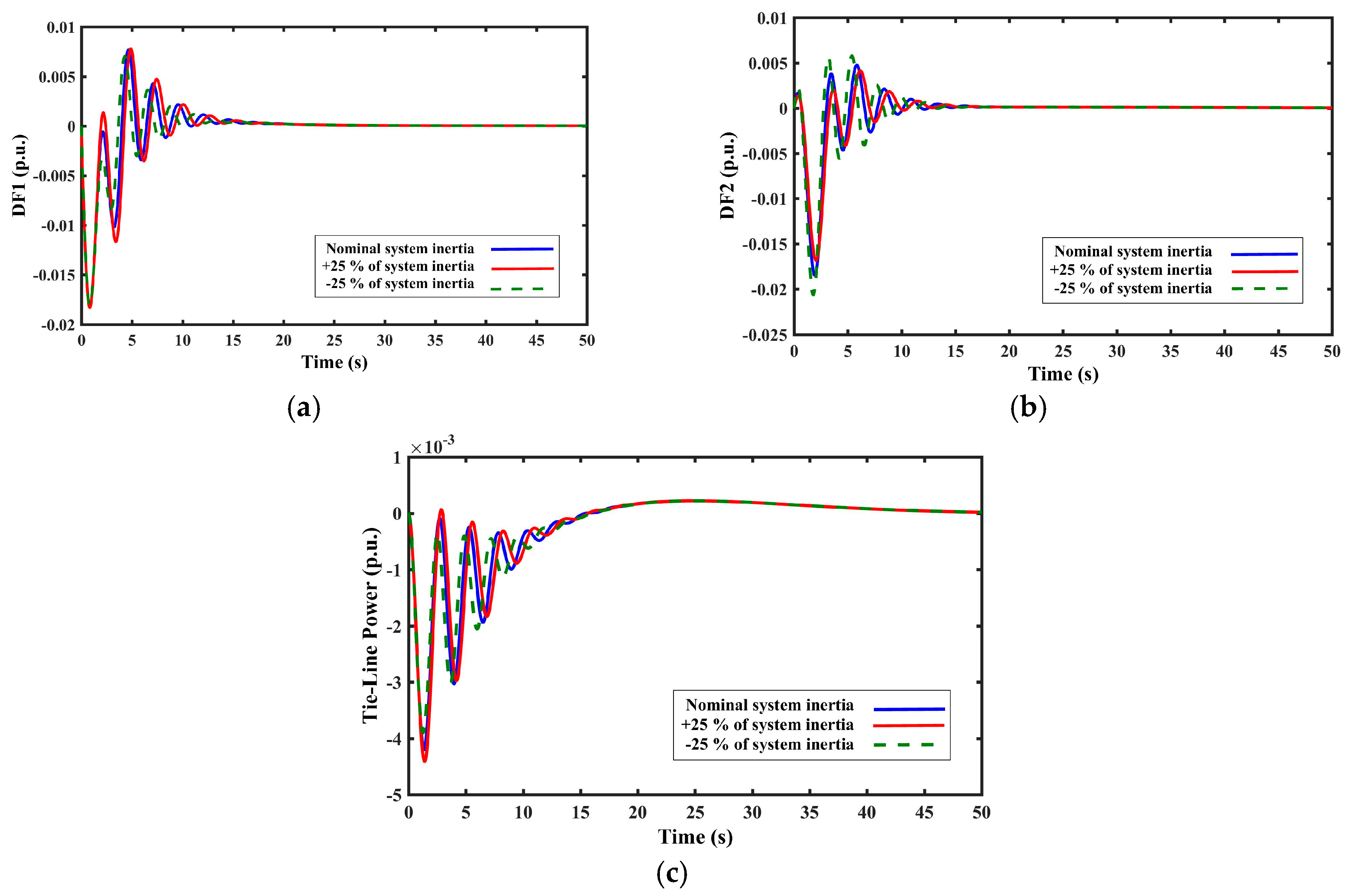
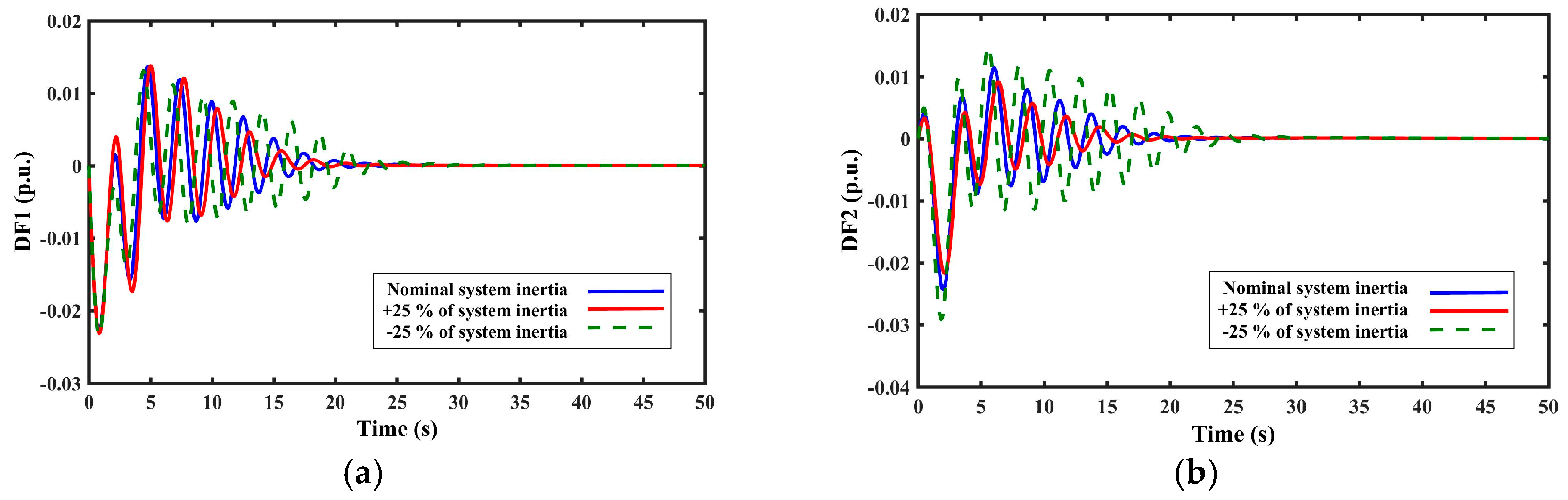
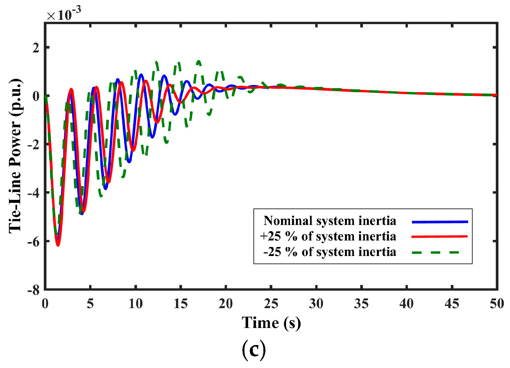
• Reliable performance for sensitivity analysis of the inertia parameter.

The remainder of this paper is comprised of four sections. Following the Introduction, the modelling method of EVs and HPs is described in Section 2. In addition, the study of the EV-HP integrated hybrid power system is given in this section. The design procedure of the FOPID controller optimized by SCA is explained in Section 3. The performance evaluation of the proposed FOPID controller through simulation results is interrogated in Section 4. Finally, the conclusion in Section 5 closes the paper.

2. System Modelling

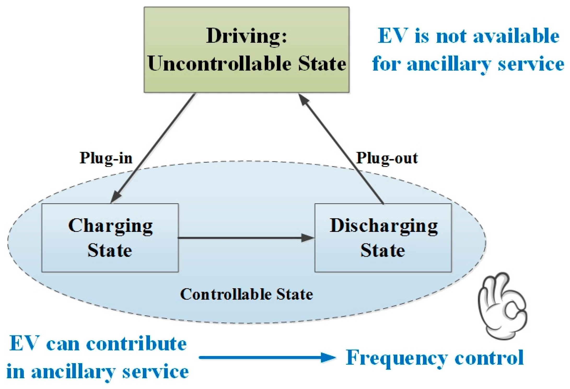
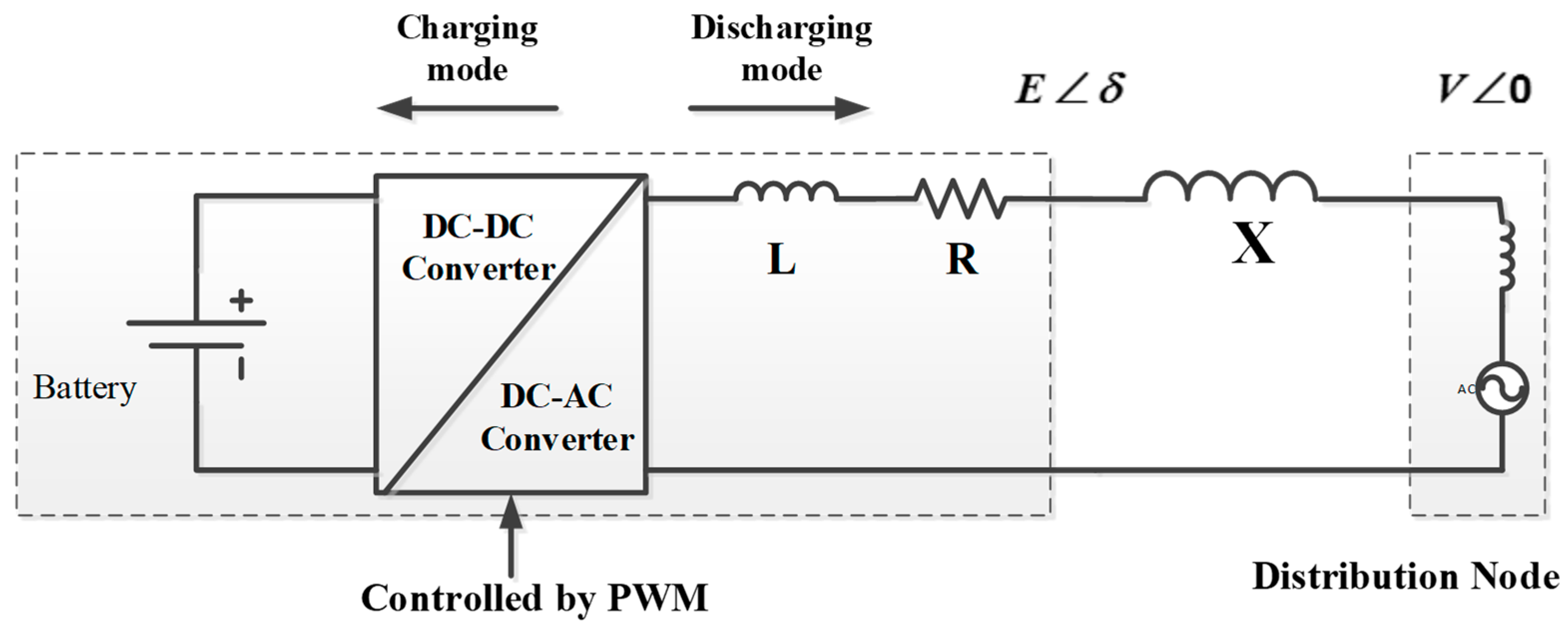
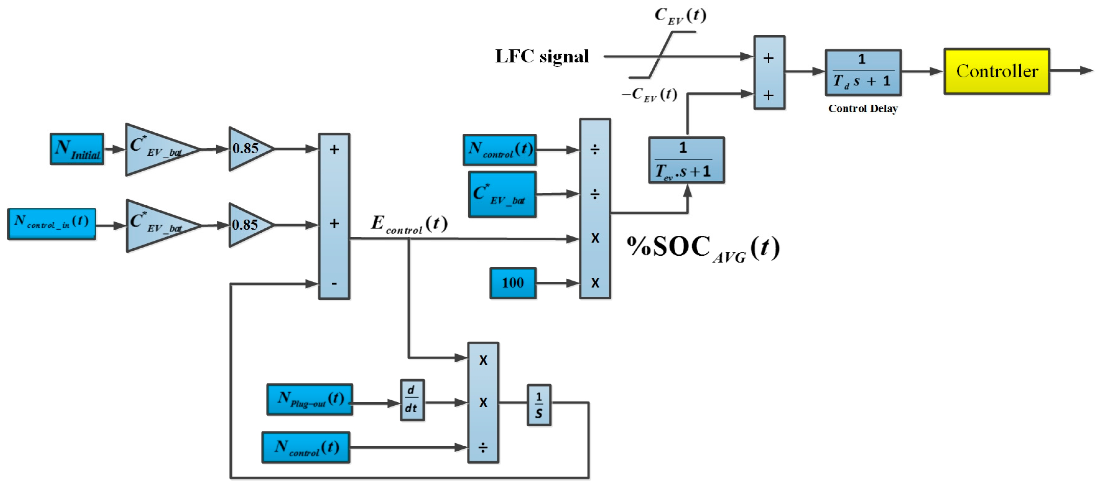
2.1. Modelling of EVs

The bidirectional connection capability of converters in EVs’ structure has made them a secure backup for frequency support in power systems. Hence, the EVs could affect the frequency performance in both charging and discharging states. The state transition property of the EVs to contribute to the LFC structure is shown in Figure 1.

As demonstrated, EVs can be controlled in charging and discharging states. However, utilization of EVs in the charging state for frequency control can reduce the useful life of their batteries. Hence, it is more rational to use EVs in the discharging state for the purpose of frequency control. By plugging in the EVs, the SOC of their batteries will be fully charged in a few hours due to the lesser driving distance of users [16].

2.1.1. SOC Concept of an EV

The SOC of an EV can be defined by exhibiting the battery and bidirectional charger diagram connected to a grid [25]. As can be seen, Figure 2 illustrates this structure in which the bidirectional converter is coupled with a distribution grid.

The power of the battery can be determined as follows:

$$S_{EV}=V{I}^{*}$$

(1)

where V is the voltage of the node and I is the current supplied by the battery, which can be calculated as follows:

$$I=\frac{E\angle \delta -V\angle 0}{jX}$$

(2)

where E, δ and X are the voltage in the terminal, the angle between V and E and the line reactance between the converter and the distribution node. The active power can be calculated as [19]:

$$P_{EV}=\frac{E\times V\sin \left(\delta \right)}{X}$$

(3)

Furthermore, it has been assumed that the considered pulse-width modulation (PWM) switching technique controls the converter so that the reactive power of the EV becomes zero (Q_EV = 0). The fast dynamics of converters are not modelled in the simulations. Therefore, the SOC of the EV can be calculated as follows [19]:

$$\mathrm{SOC}=\frac{P_1-P_2}{P_1}$$

(4)

where P₁ is the battery capacity and P₂ is the output capacity.

As is obvious, the active power exchanged between the grid and the EV’s battery could be presented by a differential equation. This is why the frequency model of EVs is made using the first-order lag function with a time constant T_ev. The time constant of EV and the first-order transfer function for modelling the delay of EV can be calculated as follows:

$$\begin{array}{l}{T}_{ev}=\frac{L}{R}\\ G\left(s\right)=\frac{1}{T_{ev}·s+1}\end{array}$$

(5)

2.1.2. Lumped Model of EVs

The lumped model of EVs in this paper is a modified version of the lumped model in [16]. The application of this model requires smart construction and control centres in the power system. The controllable EVs are defined as the EVs charged up to 80% of SOC. Furthermore, the EVs with an SOC larger than 80% are controlled in the range of 85 ± 5% of SOC. The purpose of these selections can be described as follows:

• The minimum range, which is 80%, is defined to consider the satisfaction of the EV users. The users wish to use their EVs at a high SOC level for the next trip.
• The maximum range, which is 90%, is defined to consider the lifetime of the battery. It is well known that the charging and discharging states of batteries near 100% SOC can result in deteriorated efficiency and decreased lifetime.

It is assumed that the converter of each EV has a capacity of about 30 kW to discharge in the system. From these explanations, Figure 3 exhibits the lumped model of EVs considered in this paper. From this configuration, the average SOC in a multi-area power system can be calculated to be used in frequency control.

In this model, the SOC of the lumped EVs is calculated from the existing data from different dispatching centres in the network. In the considered model, C_EV (t) is the total inverter capacity of the controllable EVs and can be defined by (6):

$$\begin{array}{l}{C}_{EV}\left(t\right)=N_{control}\left(t\right)·C_{EV-inv}^{*}\\ N_{control}\left(t\right)=N_{initial}+N_{control-in}\left(t\right)-N_{plug-out}\left(t\right)\end{array}$$

(6)

where N_control (t) and N_initial are the number of the controllable EVs and the initial number of the controllable EVs, N_control−in (t) illustrates how often the EVs are controlled and N_plug−out (t) illustrates how often the EVs are unplugged. Furthermore, the other parameters in Figure 3 can be defined as: C*_EV−bat (t) is the average battery capacity of the EVs; T_d, T_ev and E_control (t) are the communication delay, the EV’s time constant and the total stored energy of the controllable EVs. The SOC_AVG (t) can be mathematically written as follows:

$${\mathrm{SOC}}_{AVG}\left(t\right)=100\times \frac{E_{control}\left(t\right)}{N_{control}\left(t\right)·C_{EV-bat}^{*}}(\%)$$

(7)

After modelling the SOC of the lumped EVs, the main controller should be added to the model for the purpose of efficient frequency control. The controller block in Figure 3 demonstrates the main controller of EVs in the LFC structure.

2.2. Modelling of HPs

The HPs are used to supply the necessary hot water of homes. There is a tank to store hot water of a determined volume. The standard type of HP consumes 4 kW to heat 370 L of water between 55 °C in summers and 85 °C in winters. The penetration level of these appliances has increased nowadays. In 2008, the number of HPs was about two million; also, for 2020, it is expected that the number of connected HPs will be 10 million [16]. The power consumption of HPs during the heating process can be controlled. Regarding this issue, researchers can concentrate on HPs as efficient controllable loads for frequency control purposes. To model the HPs, a first-order lag transfer function can be utilized [26] in the LFC studies.

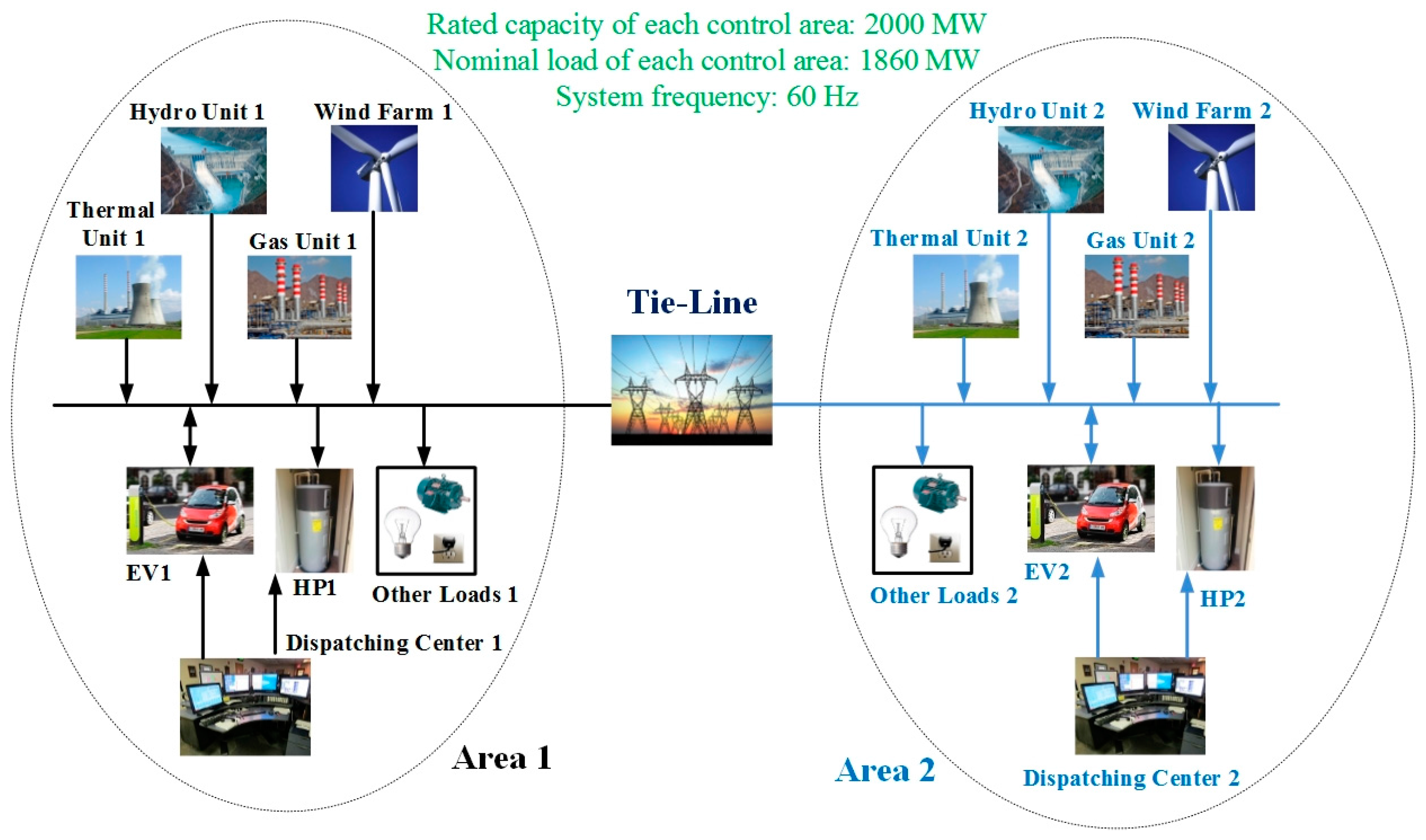
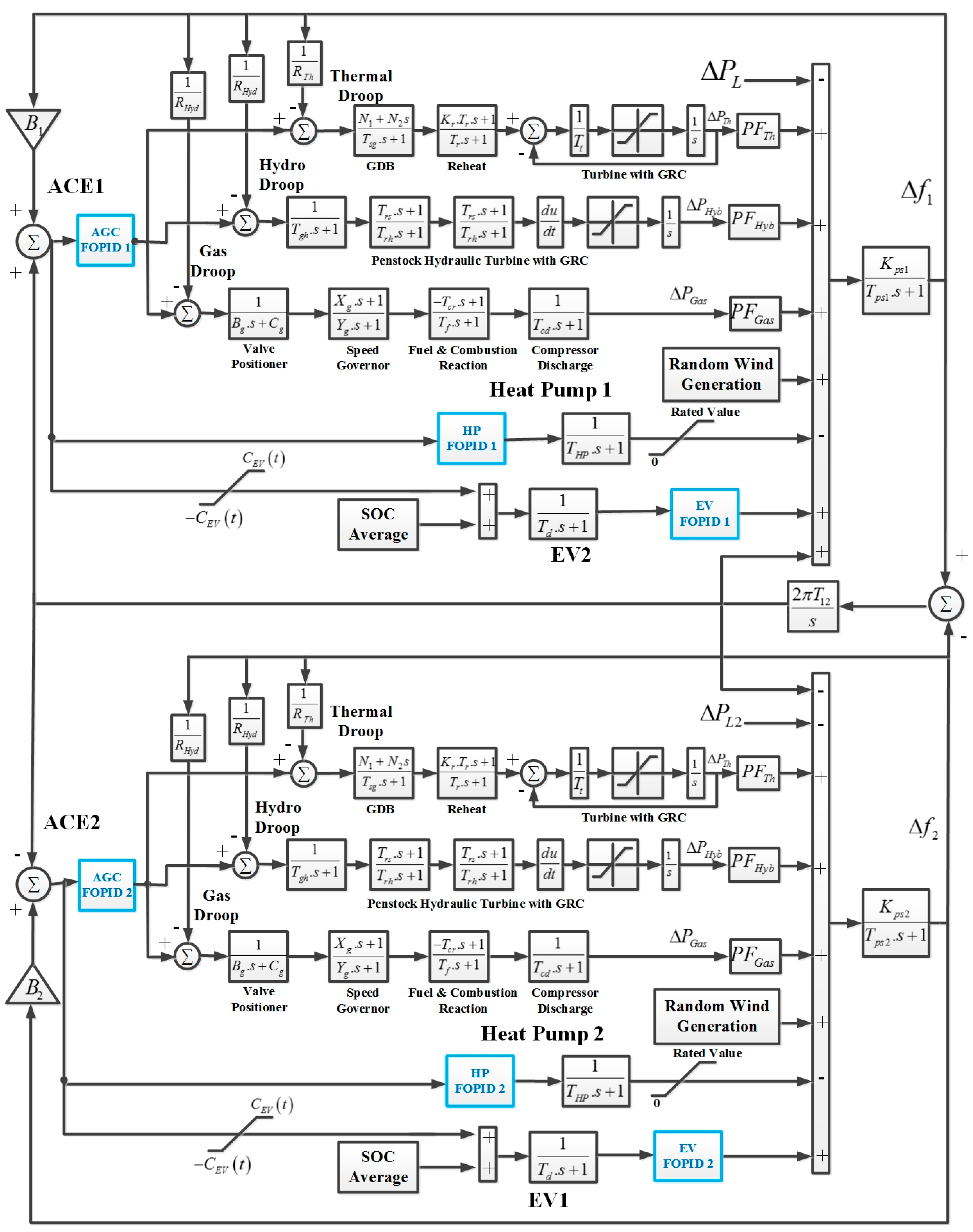
2.3. Power System under Study

A hybrid two-area power system is considered as the test bed in this paper to study the performance of the proposed controller. A schematic diagram of the considered power system is demonstrated in Figure 4. There are four generation units consisting of wind farm, reheat thermal, gas and hydro power plants in each area. As illustrated, EVs and HPs as controllable loads are connected to each area. Furthermore, general loads are connected in Area 1 and Area 2. Moreover, dispatching centres are responsible for providing adequate data about the controllable loads in each control area. The areas are connected via a tie-line, which is responsible for the power exchange between them.

In spite of the complicated and nonlinear simulation of power systems in dynamic investigations, a simplified and linear model can satisfy the analysis of frequency performance [27,28]. The linear transfer function-based model of the considered power system is depicted in Figure 5. The parameters definition of the test case are given in Nomenclature and their values are given in Appendix A. To be more adequate, the physical constraints of the generation rate (GRC) nonlinearity and governor dead-band (GDB) are included. The aim of these considerations is to validate the performance of the proposed controllers and to obtain precise and realistic simulation results. As demonstrated, the two areas are connected through a tie-line. In this figure, T_HP is the time constant of HP, and it is assumed as 0.1 s. Furthermore, T_d is the time constant of EVs, which is assumed as 0.15 s [16]. There are six FOPID controllers for EVs, HPs and AGC in the system. The design process of the FOPID controller and optimal tuning of its parameters are described in the next section.

3. Design Procedure of the FOPID Controller

3.1. A Brief Glossary on Fractional Order Calculus

The main concept behind fractional order calculus (FOC) is the extension of integer order integration and differentiation to any arbitrary real number, non-integer powers of integration and differentiation or the fractional order operator. Mathematically, this operator can be written as follows:

$$a^{D_t^{\alpha }}=\{\begin{array}{l}\raisebox{1ex}{$d^{\alpha }$}\!\left/ \!\raisebox{-1ex}{$d{t}^{\alpha }$}\right.,\Re \left(\alpha \right)>0\\ 1,\Re \left(\alpha \right)=0\\ {\displaystyle {\int }_a^t{\left(d\tau \right)}^a,\Re \left(\alpha \right)<0}\end{array}$$

(8)

In Equation (8), $a$ and t are the limits of the operation, and the fractional order is marked by α as a complex number. Generally, the definition and approximation methods for FOC should be defined. Regarding the definition, there are some methods to definite the FOC process, including Grünwald–Letnikov (G-L), Riemann–Liouville (R-L) and Caputo. In this context, the R-L definition method is more common, and its definition for the derivative section of FOC can be defined as follows:

$$a^{D_t^{\alpha }}f\left(t\right)=\frac{1}{\mathsf{\Gamma }\left(n-\alpha \right)}\frac{d^n}{d{t}^n}{{\displaystyle {\int }_a^t\left(t-\tau \right)}}^{n-\alpha -1}f\left(\tau \right)d\tau$$

(9)

In (9), $\mathsf{\Gamma }(.)$ is Euler’s gamma function, n is an integer and $a$ can be specified by $n-1\le \alpha \le n$. Furthermore, the R-L definition for the integral section of FOC can be given by (10).

$$a^{D_t^{-\alpha }}f\left(t\right)=\frac{1}{\mathsf{\Gamma }\left(\alpha \right)}{{\displaystyle {\int }_a^t\left(t-\tau \right)}}^{\alpha -1}f\left(\tau \right)d\tau$$

(10)

Moreover, the Laplace transformation, which is more typical for the explanation of the R-L definition, is given by (11) for both sections of the R-L definition.

$$L\left\{a^{D_t^{\alpha }}f\left(t\right)\right\}=s^{\alpha }F\left(s\right)-{\displaystyle \sum _{k=0}^{n-1}{s}^k{a}^{D_t^{\alpha -k-1}}f\left(t\right)}{|}_{t=0},n-1\le \alpha \le n$$

(11)

Herein, $L\left\{f\left(t\right)\right\}$ is the Laplace transform statement of $f\left(t\right)$. As a consequence, the dynamic behaviour of an FOC-based described system rises to transfer functions with a fractional order of “s” when the zero initial conditions are assumed.

On the other hand, for the purpose of approximation, there are some other approaches including Crone, Carlson, Matsuda, high or low frequency continued fraction approximations. In this paper, the Oustaloup method as known from Crone is utilized for the FOPID controller. This approximation uses high order analogue filters to approximate the fractional order differential term $S^{\alpha }$, which can be represented as:

$$S^{\alpha }=K{\displaystyle \prod _{n=1}^N\frac{S+{\omega }_k^{\prime }}{S+{\omega }_k}}$$

(12)

where N is the number of poles and zeroes. The evaluation of frequencies of poles and zeroes and also the gain of the filter can be represented respectively by:

$${\omega }_k={\omega }_b{\left(\raisebox{1ex}{${\omega }_h$}\!\left/ \!\raisebox{-1ex}{${\omega }_b$}\right.\right)}^{\frac{k+N+\raisebox{1ex}{$1$}\!\left/ \!\raisebox{-1ex}{$2$}\right.\left(1+\alpha \right)}{2N+1}}; {\omega }_k^{\prime }={\omega }_b{\left(\raisebox{1ex}{${\omega }_h$}\!\left/ \!\raisebox{-1ex}{${\omega }_b$}\right.\right)}^{\frac{k+N+\raisebox{1ex}{$1$}\!\left/ \!\raisebox{-1ex}{$2$}\right.\left(1-\alpha \right)}{2N+1}}; K={\omega }_h^{\alpha };$$

(13)

As stated earlier, $a$ is the fractional order. Furthermore, (2N + 1) is the order of the considered approximation filter. Generally, a trade-off exists between the complication of the FOC realization and accuracy. Moreover, a fifth-order Oustaloup recursive approximation is assumed within the frequency range of $\omega \in \left({10}^{-2},{10}^2\right)$ rad/s for the design process of the FOPID controller in this research.

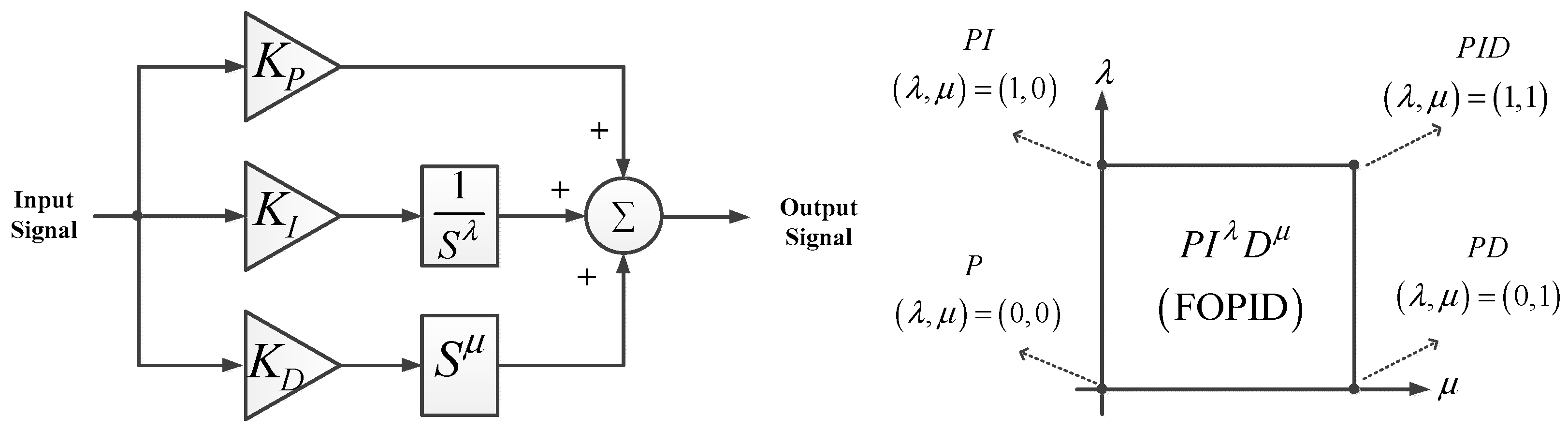
3.2. Fractional Order PID Controller

Generally, PID controllers because of their uncomplicated structure and simple design process are the most utilized controllers in industry. Despite the appealing features of simple PID controllers, they may lose their efficient performance with disturbances. This is the reason for the endeavours to examine other control methods like intelligent [29] and robust [30] controllers in the LFC structure. Recently, the fractional order concept in the design process of PID controllers has attracted much attention [31,32,33]. In [31], the FOPID controller is utilized in a hybrid power system to improve frequency oscillation damping. In [32], it is demonstrated that the FOPID controllers have more flexibility, and they are able to simultaneously satisfy multiple conflicting design objectives for a wider dynamic range than the simple PID structure, which traditionally is used in the industry. Furthermore, as another attempt, in [33], an FOPID controller was designed for a single-area LFC for all three types of turbines, including non-reheated, reheated and hydro turbines.

The general form of FOPID controllers is depicted in Figure 6 and mathematically represented as:

$$P{I}^{\lambda }{D}^{\mu }=K_P+\frac{K_I}{S^{\lambda }}+K_D{S}^{\mu }$$

(14)

In (14), K_P, K_I and K_D represent the proportional, integral and differential gains of the FOPID controller respectively. Furthermore, λ and µ denote the fractional order operators, which are often adjustable in the range of (0, 1). As demonstrated in Figure 6, the FOPID controller can performs like various models of a simple PID controller by selecting zero and one for λ and µ.

It can be recognized from (14) that there are five parameters for each FOPID controller, which should be optimized by different control methods. Recently, optimization methods have been utilized for optimizing issues in LFC problems [34]. In this study, the SCA is utilized for optimization of the FOPID controller. For this purpose, the objective function and adjustable parameters of the controllers should be determined.

3.3. Problem Formulation for the Optimization Process

In this paper, the FOPID controllers are optimized by SCA and utilized for EVs, HPs and AGC in each area of the power system. To perform a comparison of the SCA-optimized FOPID controller, the SCA-optimized simple PID controllers are also utilized for EVs, HPs and the AGC system in each area. In order to improve the frequency performance of the considered two-area power system and enhance the tie-line power exchange between the areas, the integral of time multiplied squared error (ITSE) performance index as written in (15) is selected as the objective function:

$$\text{ITSE}={\displaystyle {\int }_0^{T_S}t\left[\Delta f_1^2+\Delta f_2^2+\Delta P_{12}^2\right]}dt$$

(15)

where T_S is the simulation time. It can be simply grasped that the ITSE performance index benefits from both the integral of squared error (ISE) and the integral of time multiplied absolute error (ITAE) performance indices, as it employs squared error and time multiplication to mitigate large deviations and to reduce long settling times.

The adjustable parameters of the coordinated controllers are optimized simultaneously via minimizing the ITSE index subject to constraints. There are three parameters in simple PID controllers and five parameters in FOPID controllers that should be optimized. The constraints for a sample FOPID controller are shown below, and this can be assumed for all of the FOPID controllers.

$$\begin{array}{l}{K}_P^{\min }\le K_P\le K_P^{\max },K_I^{\min }\le K_I\le K_I^{\max }\\ K_D^{\min }\le K_D\le K_D^{\max },0\le \lambda \le 1,0\le \mu \le 1\end{array}$$

(16)

It should be noted that the three parameters of a simple PID controller are the previously-described proportional, integral and differential parameters. The range of parameters is determined by the knowledge of experts about the main system and the SCA optimization method.

3.4. Sine Cosine Algorithm

Developed by Mirjalili [35], the sine cosine algorithm (SCA) is a new population-based optimization method for solving optimization problems. The optimization process in SCA is based on a set of random solutions that applies sine and cosine functions based on the mathematical model to fluctuate away from or towards the best solution. SCA has two phases named exploration and exploitation in the optimization process. To establish exploration and exploitation of the search space for the rapid achievement of the optimal solution, this algorithm uses many random and adaptive variables. The position updating equation related to any search agent $X_i$ can be written as follows:

$$X_i^{t+1}=\{\begin{array}{l}{X}_i^t+r_1\times \sin (r_2)\times \left|r_3{P}_i^t-X_i^t\right|r_4<0.5\\ X_i^t+r_1\times \cos (r_2)\times \left|r_3{P}_i^t-X_i^t\right|r_4\ge 0.5\end{array}$$

(17)

$$r_1=c-t\frac{c}{T}$$

(18)

where $X_i^t$ and $P_i^t$ are the position of the current solution and the position of the best solution in the $j\mathrm{th}$ dimension at the $t\mathrm{th}$ iteration, respectively. $r_1,r_2,r_3$ and $r_4$ are random numbers. $r_1$ is a control parameter that states the next position, which could be either in the space between the solution and destination or outside. Furthermore, in (18), t is the current iteration, T is the maximum number of iterations and c is a constant. The superiority of the SCA algorithm over other heuristic techniques (PSO, genetic algorithm (GA), etc.) has been shown in [35]. In this research, the adjustable parameters for this algorithm are considered as follows: number of iterations = 50, number of search agents = 10 and c = 2.

4. Numerical Studies and Discussion

As discussed earlier, a hybrid two-area power system is selected as the system under study. Each area consists of four different generation units including gas, hydro, wind and reheat thermal power plants. The controllable loads (EVs and HPs) are connected to each area and equipped with the FOPID controller. To be more accurate, the simulation data about the EVs are obtained from [16]. In order to have an effective SOC, the numbers of N_control (t), N_initial and N_plug-out (t) are selected so as to produce the SOC in the range of 80–90%. Furthermore, the optimized parameters by SCA are demonstrated in

Table 1. Optimized parameters by the sine cosine algorithm (SCA) algorithm. AGC: automatic generation control; FOPID: fractional order proportional integral differential; EV: electric vehicle; HP: heat pump.

Controller Type	Areas	${\mathit{K}}_{\mathit{P}}$	${\mathit{K}}_{\mathit{I}}$	${\mathit{K}}_{\mathit{D}}$	λ	μ
FOPID-EV	Area 1	0.9884	−49.5249	0.7378	0.6704	0.6544
FOPID-HP	Area 1	0.6021	4.0225	0.699	0.4755	0.5298
FOPID-AGC	Area 1	0.9123	0.3865	0.5927	0.7014	0.6839
PID-EV	Area 1	0.8382	−33.0185	0.4237	-	-
PID-HP	Area 1	0.7707	−29.1804	0.359	-	-
PID-AGC	Area 1	0.8544	0.2979	0.584	-	-
FOPID-EV	Area 2	0.2218	−27.2737	0.382	0.454	0.4059
FOPID-HP	Area 2	0.7942	2.9808	0.2378	0.4235	0.382
FOPID-AGC	Area 2	0.5284	0.2517	0.232	0.5012	0.4631
PID-EV	Area 2	0.5465	−42.1408	0.2954	-	-
PID-HP	Area 2	0.4119	−40.1123	0.1785	-	-
PID-AGC	Area 2	0.4811	0.2977	0.5133	-	-

. As illustrated, each FOPID controller has five parameters, and each simple PI controller has three parameters, which are optimized by the SCA.

To validate the performance of the proposed FOPID controller optimized by SCA, four scenarios are investigated. The simulations are fulfilled in MATLAB/Simulink software. As the first scenario, a step load change is investigated. In the second scenario, the performance of the proposed controller is studied for a random load change, which is common in power systems. For both scenarios, the frequency performance, output power generation of conventional generators and tie-line power are shown. As the third scenario, the frequency performance and tie-line active power are investigated in an aggregated scenario including intermittent power generation of wind turbines and load changes. Eventually, a sensitivity analysis is been done in the fourth scenario.

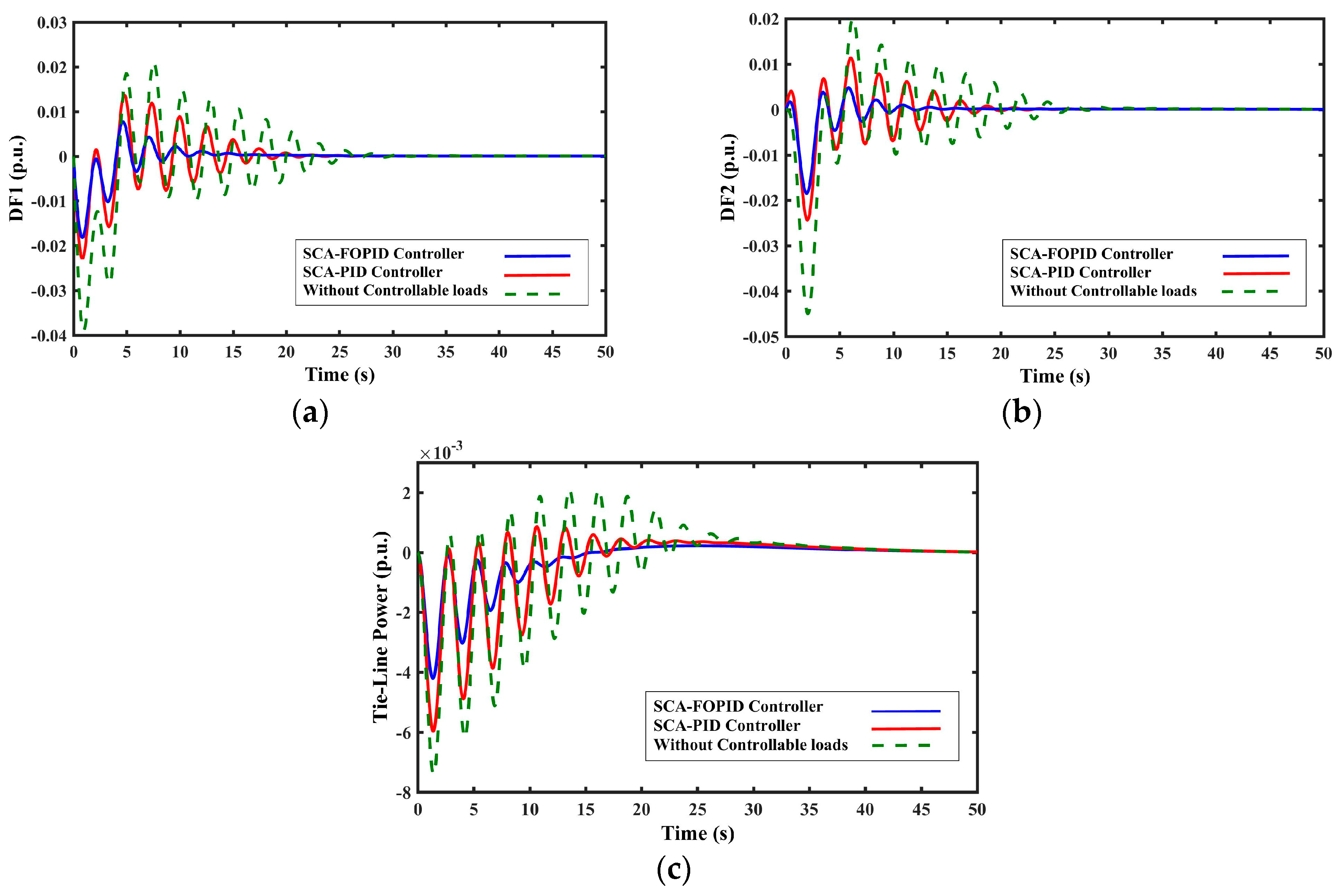
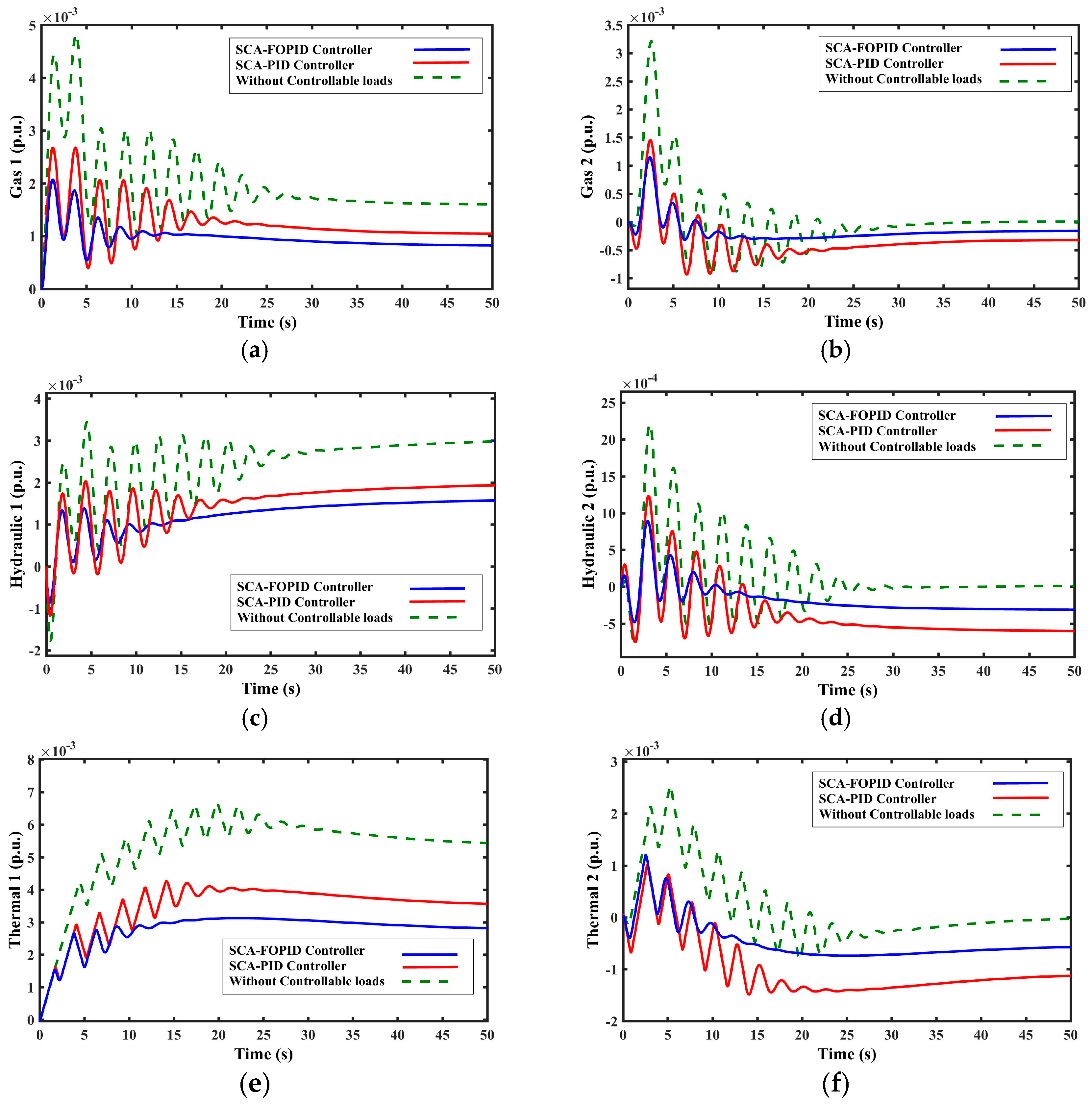
4.1. First Scenario: Step Load Change

As the first scenario, the performance of the SCA-based FOPID controller is investigated under a 0.01 p.u. step load change in area 1. Following this disturbance, the frequency performance of two areas and tie-line active power are demonstrated in Figure 7.

As shown, the proposed SCA-based FOPID controller is compared with the simple PI controller, again optimized by SCA, and the condition that there are no controllable loads in the considered power system. As can be seen, the frequency performance of the FOPID controller is better than the other conditions. In addition, the oscillations of tie-line active power are rather damped by the FOPID controller. For this scenario, the output power of generation units is investigated for the FOPID controller in comparison with the two other conditions. Figure 8 exhibits the output power deviation of gas, hydro and thermal generation units after the disturbance. The salient feature of the proposed FOPID is the better damping performance in the whole of the generation units. It is a well-known fact that oscillations can deteriorate the shaft performance in the long term. Furthermore, as depicted, by applying the FOPID controller, the increment of the generation rate of conventional units in the load has decreased.

To better demonstrate the efficiency of the proposed FOPID controller in the step scenario,

Table 2. Frequency deviation and tie-line power characteristics of FOPID, PID and AGC alone. ITSE: integral of time multiplied squared error.

Controller Type	Signal	MDR	PO	PT	ST	ITSE
FOPID EV, HP and AGC	$\Delta f_1$	0.1914	0.82	0.8265	15.0637	0.002
	$\Delta f_2$		0.8493	1.9337	11.3998
	$\Delta P_{12}$		−0.5798	1.353	9.831
PID EV, HP and AGC	$\Delta f_1$	0.3172	1.2918	0.8457	20.2843	0.0085
	$\Delta f_2$		1.4368	2.0081	19.0228
	$\Delta P_{12}$		−0.4027	1.3988	15.9148
Just AGC	$\Delta f_1$	0.0498	2.8985	0.9309	28.1927	0.0333
	$\Delta f_2$		3.494	2.0776	27.1289
	$\Delta P_{12}$		−0.2607	1.3934	26.5925

MDR: minim damping ratio, PO: peak overshoot, PT: peak time, ST: settling time.

demonstrates the damping ratios, ITSE performance index, peak overshoot, peak time and settling time of frequency deviations in Areas 1 and 2 and also the tie-line active power for the first scenario. As exhibited, the ITSE performance index has the minimum value for the case of the FOPID controller. In addition, the peak overshoot, peak time and settling time have decreased after utilization of the considered controller.

The obtained results from the step load change scenario for the FOPID controller can be summarized by the following comments:

• Decreasing the peak value of frequency and tie-line power deviations;
• Fast damping of oscillations in tie-line power deviations;
• Reduction of the generation rate in generation units;
• Better performance indices compared to the PID controller.

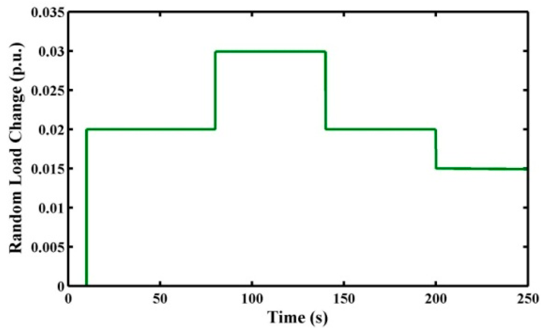
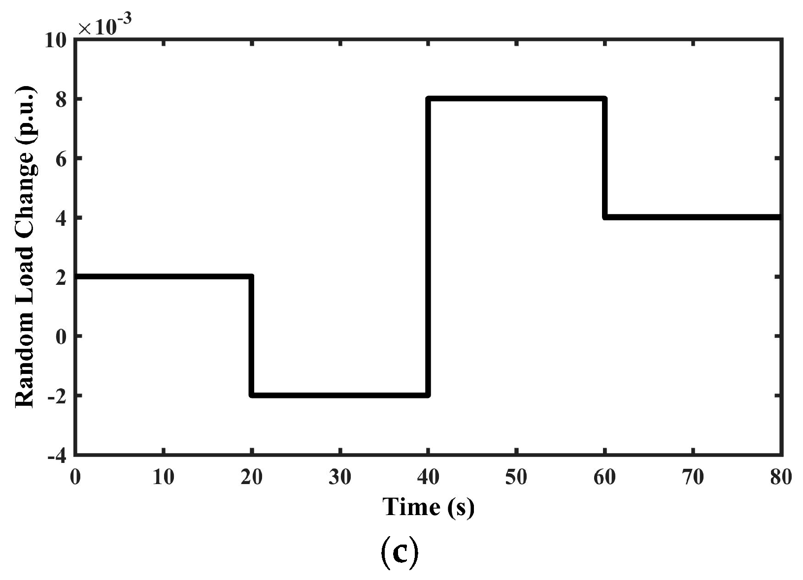
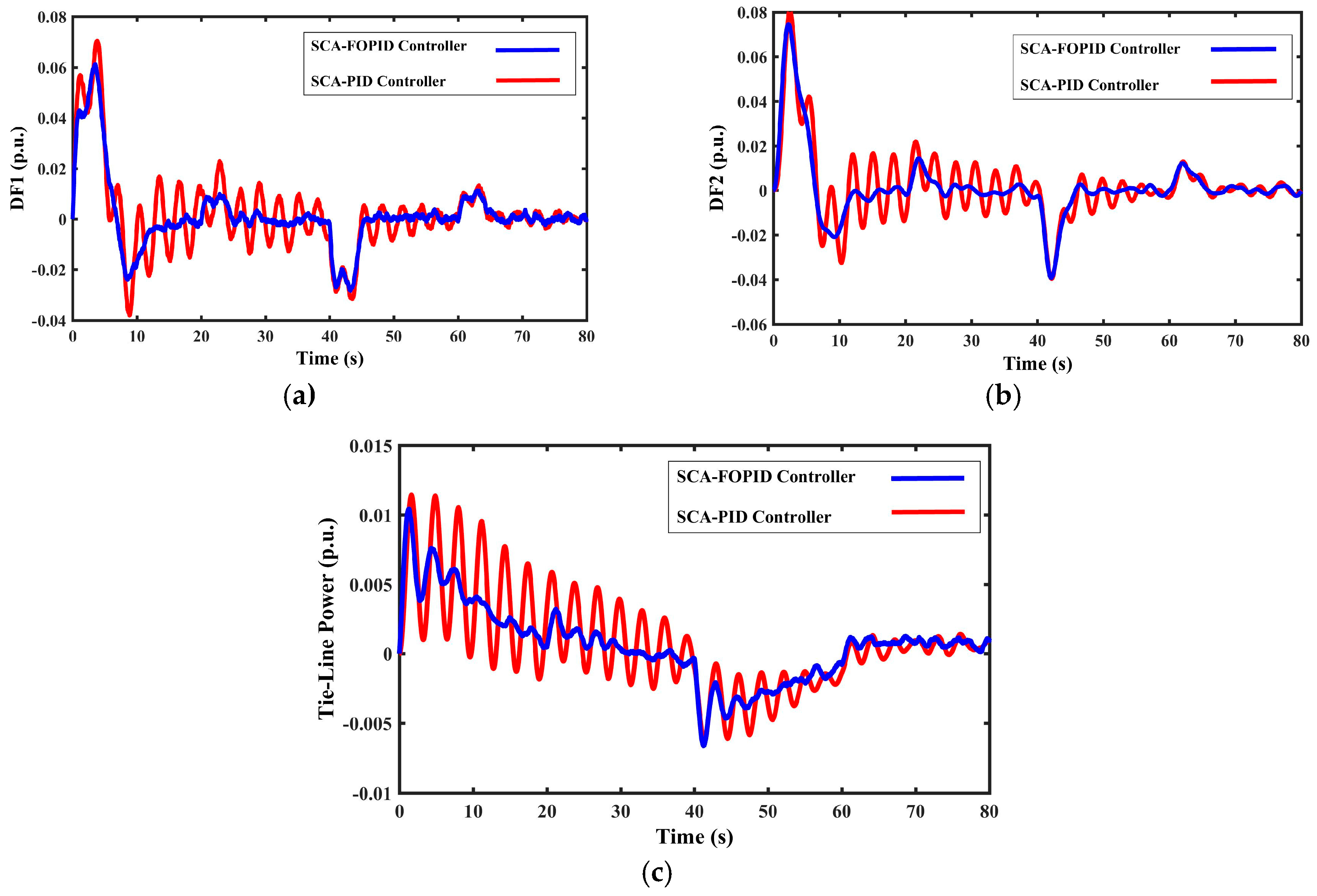
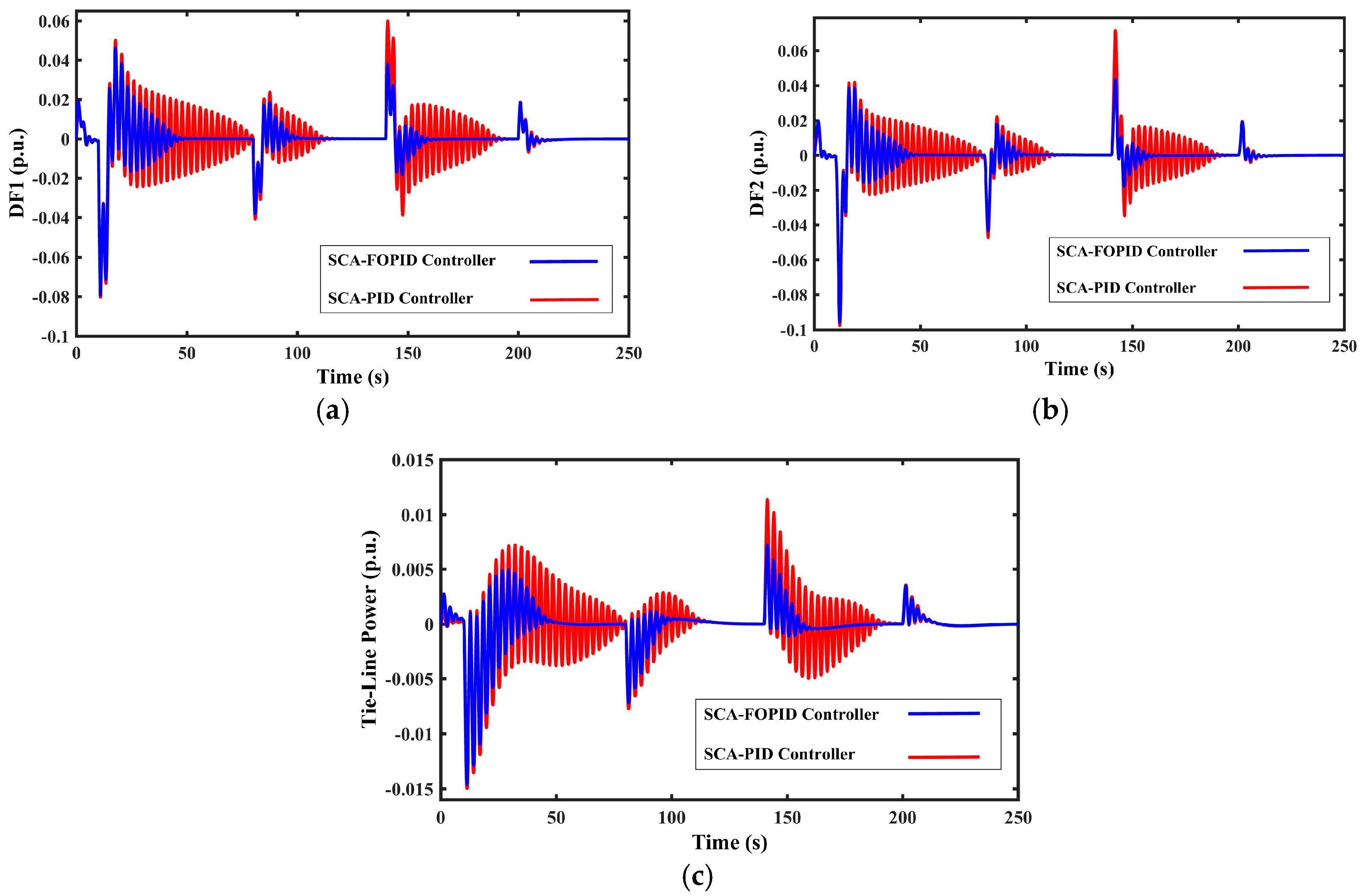
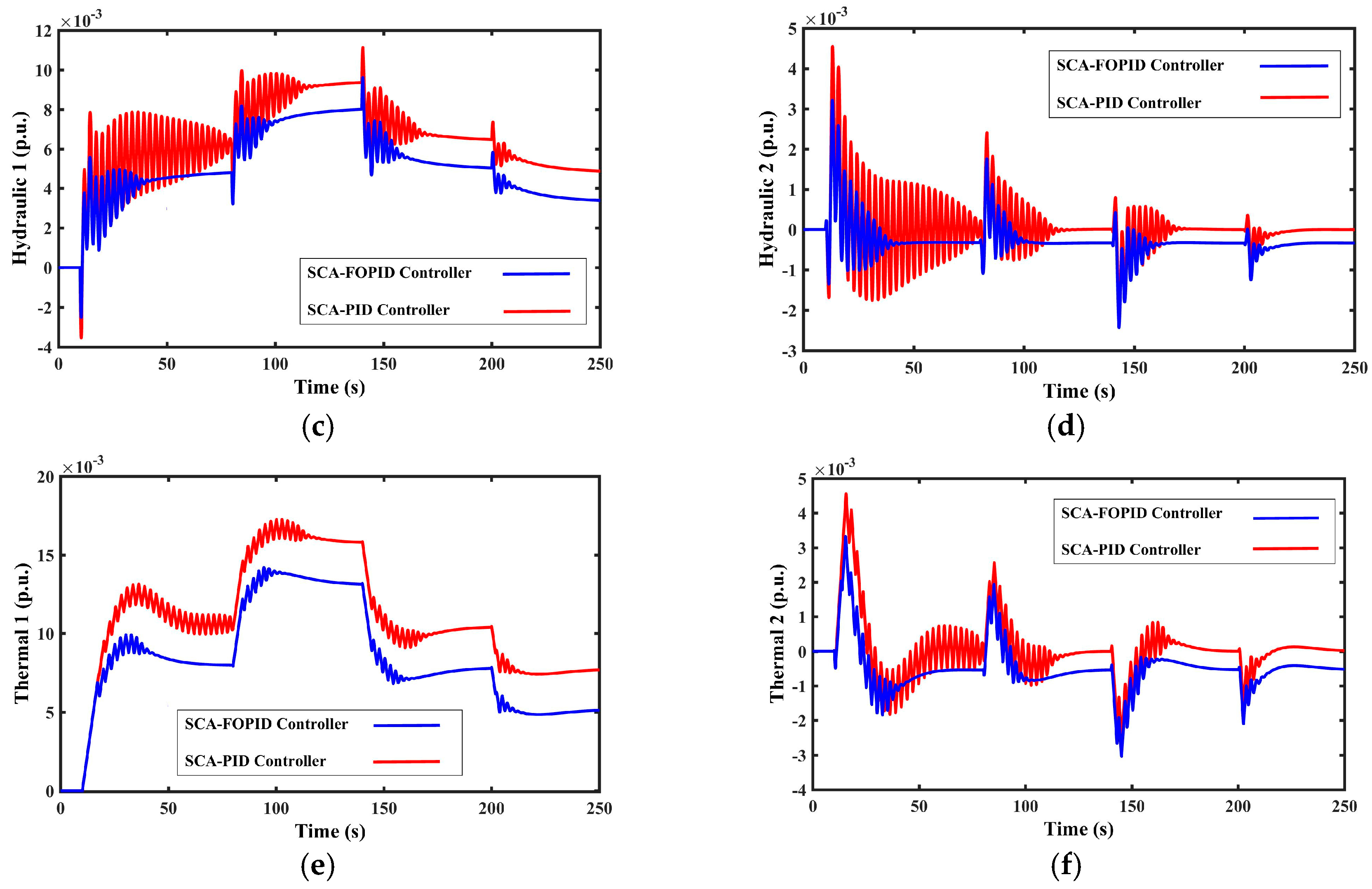
4.2. Second Scenario: Random Load Change

The optimal performance of the FOPID controller was illustrated in the previous scenario for step load change. In this scenario, to model a disturbance in demand-generation balance, a random load change as a more realistic occasion in real power systems is considered to demonstrate the tracking accuracy and damping potency of the coordinated FOPID controller for EVs, HPs and AGC. This random load change is depicted in Figure 9.

Following the mentioned random load variation, the frequency performance of Areas 1 and 2 and the tie-line power deviation are represented in Figure 10. In this case, the performance of the FOPID controller is compared with the simple PI controller. This is so because of the weak performance of the power system without controllable loads. Although the simulated disturbance is more complicated than the first one, the FOPID controller is more robust than the simple PI controller. The robustness of the FOPID is obvious, and also, the frequency deviations are damped rapidly after the load changes. In a similar manner, the FOPID has stabilized the tie-line power.

Similarly, the output power performance of generation units is exhibited in this scenario. Figure 11 demonstrates their performance following the random load change. As can be seen, the FOPID controller has stabilized the output oscillation of conventional units more rapidly. Furthermore, the generated power is decreased for all the cases by utilization of the proposed controller. The near unstable behaviour of generation rates in the generation units may be because of low inertia in the system for the both PID and FOPID controllers. However, it is more because of the basis of the scenario. In this scenario, the load of the system changes quickly, and the generation units do not have appropriate time to recover their generation rates completely. Therefore, it seems that the generation rates are near unstable for this scenario.

The obtained results from the random load change scenario can be summarized by the following comments:

• Good frequency tracking after load changes in the system;
• Desirable oscillation damping due to;
• Reduction of the generation rate in generation units.

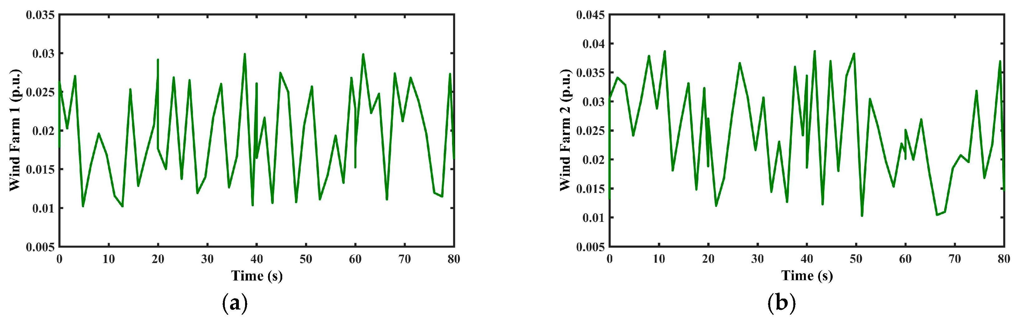
4.3. Third Scenario: Intermittent Generated Power by Wind Farm and Load Change

As the third scenario, the intermittent generated power of wind farms and load change are investigated simultaneously, and the performance of the SCA-based FOPID controller for EV, HP and AGC is analysed. Figure 12 indicates the rendered power from wind farms to Areas 1 and 2 and load change in the considered hybrid power system. As can be seen, the generated power changes constantly over time. This can conceivably affect the frequency performance of each area.

The frequency performance and tie-line power deviation after the combined disturbance are shown in Figure 13. As illustrated, the frequency and tie-line power have deviated subsequently. To be more accurate, the performance of the FOPID controller is compared with the simple PID controller again. The highly reliable performance of the FOPID controller is obvious in this scenario. To put it succinctly, the FOPID controller can mitigate the intermittent functionality of renewable energy sources efficiently. The obtained results from this aggregated scenario can be summarized as the SCA-based FOPID controller has good behaviour following the intermittent generation of renewable energy resources.

4.4. Fourth Scenario: Inertia Deviation Analysis

As the last scenario, sensitivity analysis is carried out to examine the robustness of the controllers under inertia deviation of the power system. To do so, the T_ps (power system time constant) of Area 2 as an indicator of the area’s inertia changed drastically by ±25% of the nominal value regarding the Scenario 1 condition. The damping responses obtained after considering the uncertainty scenario are demonstrated in Figure 14 for the SCA-based FOPID controller and in Figure 15 for the SCA-based PID controller. Furthermore, the performance indices are listed in

Table 3. Frequency deviation and tie-line power characteristics of FOPID and PID controllers for ±25% variations in the power system time constant.

Controller Type	Signal	MDR	PO	PT (s)	ST (s)	ITSE
FOPID EV, HP and AGC $+25\%$	$\Delta f_1$	0.157	0.8296	0.8265	15.692	0.0021
	$\Delta f_2$		0.6827	2.0474	12.0101
	$\Delta P_{12}$		−0.5588	1.4045	10.2723
FOPID EV, HP and AGC $-25\%$	$\Delta f_1$	0.2331	0.8047	0.8175	13.9472	0.0019
	$\Delta f_2$		1.0629	1.7901	12.4747
	$\Delta P_{12}$		−0.6099	1.2731	10.9536
PID EV, HP and AGC $+25\%$	$\Delta f_1$	0.299	1.3178	0.8417	18.6309	0.0069
	$\Delta f_2$		1.1718	2.1419	17.3286
	$\Delta P_{12}$		−0.3812	1.4602	12.9268
PID EV, HP and AGC $-25\%$	$\Delta f_1$	0.3408	1.3386	0.8053	24.487	0.0162
	$\Delta f_2$		1.9065	1.8441	24.6646
	$\Delta P_{12}$		−0.4284	1.2821	23.9932

MDR: minim damping ratio, PO: peak overshoot, PT: peak time, ST: settling time.

.

It can be inferred from Figure 14 and Figure 15 and Table 3 that in comparison with the nominal responses presented in Table 2 and Figure 7, the considered severe variations have negligible impacts on the damping characteristics since the damping ratios, performance indices and damping control measures deviate slightly from the nominal values, so that the power system is still stable as before. Hence, once the tuneable parameters are adjusted for nominal loading conditions and parameters, there is no need to readjust for the ±25% variations in the power system time constant.

It should be noted that the aforementioned evaluations of the coordinated SCA-based FOPID controllers are reliable theoretically with regard to the mathematical assumptions. From a practical viewpoint, the application of the FOPID controllers in the power system stability issues is an emerging solution.

5. Conclusions and Future Work

The conducted survey demonstrated the application of FOPID controller for HP, EV and AGC in a smart hybrid power system. The parameters of the proposed FOPID controller were optimized by SCA as a novel approach for optimization problems. A lumped model of EVs and a simple model of HPs were utilized in the LFC structure. The FOPID controller was employed to control the power consumption of HPs and the discharging state of EVs. The effectiveness of the designed SCA-based FOPID controller was demonstrated in four scenarios. As the first result of employing the FOPID controller, it was demonstrated that frequency deviations and tie-line power fluctuations were mitigated more efficiently compared to the PID controller. Furthermore, as the deduced result, the effect of intermittent generated power of wind farms on frequency and tie-line power deviations was moderated very effectively by the FOPID controller. Due to high cost operation and air pollution of conventional units, the proposed SCA-based FOPID controller diminished the generation rate of such units as indicated in the simulation results. Sensitivity analysis of the inertia parameter in the two-area power system demonstrated the reliability of the designed SCA-based FOPID controller.

In this research, a deregulated structure for the considered power system was neglected. To have different contributions by the power plants, there needs to be a deregulated structure by distribution companies (DISCOs) and generators. On the other hand, in the case of EVs, their contribution can be investigated by 24-h period analysis of the availability of EVs from the view point of the EV station. Frequency studies in the case of different contributions of power plants and different charging/discharging levels of EVs are different from those investigated by this research, and this requires planning investigation alongside the control design. However, such an idea as the different contributions of power plants and EVs combined with disturbances should be considered in future works.

References

1. Eremia, M.; Shahidehpour, M. Handbook of Electrical Power System Dynamics: Modeling, Stability, and Control; John Wiley and Sons: Hoboken, NJ, USA, 2013. [Google Scholar]
2. Machowski, J. Power System Dynamics: Stability and Control, 2nd ed.; John Wiley and Sons: Hoboken, NJ, USA, 2008. [Google Scholar]
3. Bevrani, H. Robust Power System Frequency Control, 2nd ed.; Springer: Berlin, Gemany, 2014. [Google Scholar]
4. Babahajiani, P.; Shafiee, Q.; Bevrani, H. Intelligent demand response contribution in frequency control of multi-area power systems. IEEE Trans. Smart Grid 2016. [Google Scholar] [CrossRef]
5. Qi, Y.; Wang, D.; Jia, H.; Pu, T.; Chen, N.; Liu, K. Frequency control ancillary service provided by efficient power plants integrated in queuing-controlled domestic water heaters. Energies 2017, 10, 559. [Google Scholar] [CrossRef]
6. Ma, K.; Yuan, C.; Yang, J.; Liu, Z.; Guan, X. Switched control strategies of aggregated commercial HVAC systems for demand response in smart grids. Energies 2017, 10, 953. [Google Scholar] [CrossRef]
7. Motalleb, M.; Thornton, M.; Reihani, E.; Ghorbani, R. Providing frequency regulation reserve services using demand response scheduling. Energy Convers. Manag. 2016, 124, 439–452. [Google Scholar] [CrossRef]
8. Mu, Y.; Wu, J.; Ekanayake, J.; Jenkins, N.; Jia, H. Primary frequency response from electric vehicles in the great Britain power system. IEEE Trans. Smart Grid 2013, 4, 1142–1150. [Google Scholar] [CrossRef]
9. Brenna, M.; Foiadelli, F.; Longo, M.; Zaninelli, D. e-Mobility forecast for the transnational e-corridor planning. IEEE Trans. Intell. Transp. Syst. 2016, 17, 680–689. [Google Scholar] [CrossRef]
10. Lotfy, M.E.; Senjyu, T.; Farahat, M.A.; Abdel-Gawad, A.F.; Matayoshi, H. A polar fuzzy control scheme for hybrid power system using vehicle-to-grid technique. Energies 2017, 10, 1083. [Google Scholar] [CrossRef]
11. Masuta, T.; Yokoyama, A.; Tada, Y. System frequency control by heat pump water heaters (HPWHs) on customer side based on statistical HPWH model in power system with a large penetration of renewable energy sources. In Proceedings of the 2010 International Conference on Power System Technology (POWERCON), Hangzhou, China, 24–28 October 2010. [Google Scholar]
12. Han, S.; Han, S.; Sezaki, K. Development of an optimal vehicle-to-grid aggregator for frequency regulation. IEEE Trans. Smart Grid 2010, 1, 65–72. [Google Scholar]
13. Izadkhast, S.; Garcia-Gonzalez Frias, P.; Ramirez-Elizondo, L.; Bauer, P. An aggregate model of plug-in electric vehicles including distribution network characteristics for primary frequency control. IEEE Trans. Power Syst. 2016, 31, 2987–2998. [Google Scholar] [CrossRef]
14. Liu, H.; Hu, Z.; Song, Y.; Lin, J. Decentralized vehicle-to-grid control for primary frequency regulation considering charging demands. IEEE Trans. Power Syst. 2013, 28, 3480–3489. [Google Scholar] [CrossRef]
15. Liu, H.; Hu, Z.; Song, Y.; Wang, J.; Xie, X. Vehicle-to-Grid Control for Supplementary Frequency Regulation Considering Charging Demands. IEEE Trans. Power Syst. 2015, 30, 3110–3119. [Google Scholar] [CrossRef]
16. Masuta, T.; Yokoyama, A. Supplementary load frequency control by use of a number of both electric vehicles and heat pump water heaters. IEEE Trans. Smart Grid 2012, 3, 1253–1262. [Google Scholar] [CrossRef]
17. Meng, J.; Mu, Y.; Jia, H.; Wu, J.; Yu, X.; Qu, B. Dynamic frequency response from electric vehicles considering travelling behavior in the Great Britain power system. Appl. Energy 2016, 162, 966–979. [Google Scholar] [CrossRef]
18. Falahati, S.; Taher, S.; Shahidehpour, M. Grid frequency control with electric vehicles by using of an optimized fuzzy controller. Appl. Energy 2016, 178, 918–928. [Google Scholar] [CrossRef]
19. Pahasa, J.; Ngamroo, I. Coordinated Control of Wind Turbine Blade Pitch Angle and PHEVs Using MPCs for Load Frequency Control of Microgrid. IEEE Syst. J. 2016, 10, 97–105. [Google Scholar] [CrossRef]
20. Vachirasricirikul, S.; Ngamroo, I. Robust LFC in a smart grid with wind power penetration by coordinated V2G control and frequency controller. IEEE Trans. Smart Grid 2012, 5, 371–380. [Google Scholar] [CrossRef]
21. Debbarma, S.; Dutta, A. Utilizing electric vehicles for LFC in restructured power systems using fractional order controller. IEEE Trans. Smart Grid 2017, 8, 2554–2564. [Google Scholar] [CrossRef]
22. Oshnoei, A.; Hagh, M.T.; Khezri, R.; Mohammadi-Ivatloo, B. Application of IPSO and fuzzy logic methods in electrical vehicles for efficient frequency control of multi-area power systems. In Proceedings of the 2017 Iranian Conference on Electrical Engineering (ICEE), Tehran, Iran, 2–4 May 2017; pp. 1349–1354. [Google Scholar]
23. Zhong, J.; He, L.; Li, C.; Cao, Y.; Wang, J.; Fang, B.; Zeng, L.; Xiao, G. Coordinated control for large-scale EV charging facilities and energy storage devices participating in frequency regulation. Appl. Energy 2014, 123, 253–262. [Google Scholar] [CrossRef]
24. Vachirasricirikul, S.; Ngamroo, I. Robust controller design of heat pump and plug-in hybrid electric vehicle for frequency control in a smart microgrid based on specified-structure mixed control technique. Appl. Energy 2011, 123, 3860–3868. [Google Scholar] [CrossRef]
25. Singh, M.; Kumar, P.; Kar, I. Implementation of vehicle to grid infrastructure using fuzzy logic controller. IEEE Trans Smart Grid 2012, 3, 565–577. [Google Scholar] [CrossRef]
26. Senjyu, T.; Tokudome, M.; Yona, A.; Funabashi, T. A frequency control approach by decentralized controllable loads in small power systems. In Proceedings of the IEEE 2nd International Power and Energy Conference (PECon 2008), Johor Bahru, Malaysia, 1–3 December 2008; pp. 1074–1080. [Google Scholar]
27. Kundur, P. Power System Stability and Control; McGraw-Hill: New York, NY, USA, 1994. [Google Scholar]
28. Zare, K.; Hagh, M.T.; Morsali, J. Effective oscillation damping of an interconnected multi-source power system with automatic generation control and TCSC. Int. J. Electr. Power Energy Syst. 2015, 65, 220–230. [Google Scholar] [CrossRef]
29. Khezri, R.; Golshannavaz, S.; Shokoohi, S.; Bevrani, H. Fuzzy Logic Based Fine-tuning Approach for Robust Load Frequency Control in a Multi-area Power System. Electr. Power Compon. Syst. 2016, 44, 2073–2083. [Google Scholar] [CrossRef]
30. Golshannavaz, S.; Khezri, R.; Esmaeeli, M.; Siano, P.L. A two-stage robust-intelligent controller design for efficient LFC based on Kharitonov theorem and fuzzy logic. J. Ambient Intell. Hum. Comput. 2017, 1–10. [Google Scholar] [CrossRef]
31. Pan, I.; Das, S. Fractional order AGC for distributed energy resources using robust optimization. IEEE Trans. Smart Grid 2015, 7, 2175–2186. [Google Scholar] [CrossRef]
32. Das, S.; Pan, I. On the mixed loop-shaping tradeoffs in fractional-order control of the AVR system. IEEE Trans. Ind. Inform. 2014, 10, 1982–1992. [Google Scholar] [CrossRef]
33. Swati, S.; Yogesh, V.H. Fractional order PID controller for load frequency control. Energy Convers. Manag. 2014, 85, 343–353. [Google Scholar]
34. Bevrani, H.; Hiyama, T. Intelligent Automatic Generation Control; CRC Press: New York, NY, USA, 2011. [Google Scholar]
35. Mirjalili, S. SCA: A sine cosine algorithm for solving optimization problems. Knowl.-Based Syst. 2016, 96, 120–133. [Google Scholar] [CrossRef]
Figure 1. The state transition of electric vehicles (EVs).
Energies 11 00420 g001
Figure 2. EV structure connected to the distribution grid. PWM: pulse-width modulation.
Energies 11 00420 g002
Figure 3. Lumped model of EVs. LFC: load frequency control.
Energies 11 00420 g003
Figure 4. Schematic diagram of the test system under study.
Energies 11 00420 g004
Figure 5. The linearized transfer function-based model of the two-area power system with controllable loads. GDB: governor dead-band; GRC: constraints of the generation rate; ACE: area control error.
Energies 11 00420 g005
Figure 6. The general structure of the fractional order proportional integral differential (FOPID) controller.
Energies 11 00420 g006
Figure 7. Frequency deviation and tie-line active power change in the first scenario: (a) frequency deviation of area 1; (b) frequency deviation of area 2; (c) tie-line power deviation. DF: frequency deviation.
Energies 11 00420 g007
Figure 8. Output power deviation of gas, hydro and thermal generation units after the step load change, (a,b) output power deviation of Gas units in area 1 and 2 respectively; (c,d) output power deviation of hydro units in area 1 and 2 respectively; (e,f) output power deviation of Thermal units in area 1 and 2 respectively.
Energies 11 00420 g008
Figure 9. Random load variation: third scenario.
Energies 11 00420 g009
Figure 10. Frequency deviation and tie-line active power change in the second scenario: (a) frequency deviation of area 1; (b) frequency deviation of area 2; (c) tie-line power deviation.
Energies 11 00420 g010
Figure 11. Output power deviation of gas, hydro and thermal units after random load change, (a,b) output power deviation of Gas units in area 1 and 2 respectively; (c,d) output power deviation of hydro units in area 1 and 2 respectively; (e,f) output power deviation of Thermal units in area 1 and 2 respectively.
Energies 11 00420 g011aEnergies 11 00420 g011b
Figure 12. Output power deviation of Wind Farms 1 and 2 and load change: (a) rendered power from wind farm 1; (b) rendered power from wind farm 2; (c) random load change.
Energies 11 00420 g012aEnergies 11 00420 g012b
Figure 13. Frequency deviation and tie-line active power change in the third scenario: (a) frequency deviation of area 1; (b) frequency deviation of area 2; (c) tie-line power deviation.
Energies 11 00420 g013
Figure 14. Frequency deviation and tie-line active power change in the fourth scenario for the SCA-based FOPID controller, (a) frequency deviation of area 1; (b) frequency deviation of area 2; (c) tie-line power deviation.
Energies 11 00420 g014
Figure 15. Frequency deviation and tie-line active power change in the fourth scenario for the SCA-based PID controller: (a) frequency deviation of area 1; (b) frequency deviation of area 2; (c) tie-line power deviation.
Energies 11 00420 g015aEnergies 11 00420 g015b