Assessment of the Joint Development Potential of Wave and Wind Energy in the South China Sea

Abstract

The South China Sea is a major shipping hub between the West Pacific and Indian Oceans. In this region, the demand for energy is enormous, both for residents’ daily lives and for economic development. Wave energy and wind energy are two major clean and low-cost ocean sources of renewable energy. The reasonable development and utilization of these energy sources can provide a stable energy supply for coastal cities and remote islands of China. Before wave energy and wind energy development, however, we must assess the potential of each of these sources. Based on high-resolution and high-accuracy wave field data and wind field data obtained by ERA-Interim reanalysis for the recent 38-year period from 1979–2016, the joint development potential of wave energy and wind energy was assessed in detail for offshore and nearshore areas in the South China Sea. Based on potential installed capacity, the results revealed three promising areas for the joint development of nearshore wave energy and wind energy, including the Taiwan Strait, Luzon Strait and the sea southeast of the Indo-China Peninsula. For these three dominant areas (key stations), the directionality of wave energy and wind energy propagation were good in various seasons; the dominant wave conditions and the dominant wind conditions were the same, which is advantageous for the joint development of wave and wind energy. Existing well-known wave energy converters (WECs) are not suitable for wave energy development in the areas of interest. Therefore, we must consider the distributions of wave conditions and develop more suitable WECs for these areas. The economic and environmental benefits of the joint development of wave and wind energy are high in these promising areas. The results described in this paper can provide references for the joint development of wave and wind energy in the South China Sea.

1. Introduction

Energy sources are the material basis for human survival. Certain fossil energy resources, such as petroleum, natural gas and coal, are very limited and will diminish in the future. In addition, the overuse of conventional fossil energy will lead to serious environment pollution. To confront energy crises and environment pollution, many countries have focused on the exploitation and utilization of renewable energy sources. There are several abundant and renewable energy sources in the oceans, including current energy, tidal energy, thermal gradient energy, ocean salinity energy, and wave and ocean wind energy. Among these types of energy, wave and wind energy have the greatest potential, and are the most valuable type of ocean energy, providing inexhaustible energy sources without carbon emissions. The rational exploitation of wave and wind energy will effectively alleviate the energy crises and environmental pollution problems.

Wave and wind energy will become very important energy sources for human society in the future. Before these energy sources can be developed, however, a reliable assessment of the temporal and spatial distributions of wave and wind energy must be performed in areas of interest to provide the basis for decisions regarding siting wave wind farms and the design and operation of wave and wind energy converters. For this reason, researchers in various countries throughout the world have conducted considerable research on assessments of wave and wind energy. In 2008, Cornett investigated wave energy in the global ocean based on WAVEWATCH-III wave model data [1]. In 2012, Arinaga and Cheung assessed wave energy in the global ocean based on 10 years of WAVEWATCH-III wave model wave field data [2]. In 2014, Zheng et al. carried out a detailed wind wave energy and swell energy assessment for the global ocean based on global wind wave and swell fields from ERA-40 reanalysis data for the most recent 45 years from the European Centre for Medium-Range Weather Forecasts (ECMWF) [3]. In 2014, Zheng et al. evaluated the temporal and spatial distributions and resources of wind energy in the global ocean using cross-calibrated Multi-Platform (CCMP) wind field data from 1988 to 2011 and established a grading atlas for wind energy for the global ocean [4]. In 2016, Zheng et al. analyzed and summarized research on wind energy assessments for the global ocean [5]. In 2017, Zheng et al. provided an overview of long-term climatic trends and medium- to long-term predictions of wave energy [6]. These previous works primarily addressed large-scale wave and wind energy in the global ocean.

However, at present, wave and wind energy development in offshore and large-scale areas are difficult and expensive, so in the most recent 10 years, small-scale wave and wind energy assessments have become areas of widespread interest in this field. From 2009 to 2011, Iglesias et al. undertook refined evaluations of wave energy for various small-scale areas around the sea areas of Spain based on a wave model [7,8,9,10,11,12]. In 2011, Kim et al. assessed wave energy in offshore deep water around the Korea Peninsula using hindcast data from 1979 to 2003 and studied wave energy in nearshore waters around Hongdo using Simulating Waves Nearshore (SWAN) data [13]. In 2014, Yamaguchi and Ishihara assessed wind climate and wind energy potential off the coast of the Kanto area in Japan using a mesoscale model [14]. In 2015, Ko et al. assessed small-scale wind energy potential in Chuuk State of Micronesia based on meteorological observation data [15]. In 2014, Fang studied nearshore wind energy potential on the west coast of Taiwan and Penghu Islands based on a mesoscale numerical weather prediction model (MM5) [16]. In 2013, Rusu and Onea assessed wind energy for the Caspian Sea using ECMWF wind data [17].

In China’s seas, which are our area of interest and are influenced by the East Asian monsoon and typhoons from the western Pacific, wave and wind energy are abundant. Chinese researchers have carried out a series of works to assess wave and wind energy in the China Sea. From 2012 to 2013, Zheng et al. studied the distributions of wave and wind energy for China’s seas based on wave field data from WAVEWATCH-III and wind field data from CCMP, which can provide references for wave and wind energy development [18,19]. In 2013, Zheng et al. analyzed wave energy at key locations in 12 regions along the coast of Taiwan based on wave buoy data [20]. In 2014, Liang et al. assessed wave energy in 2 key areas in nearshore and offshore adjacent sea areas east of China based on 22 years of wave field data simulated using the SWAN model [21]. All these works provide useful references for wave and wind energy assessments.

In this paper, our area of interest is the South China Sea, which is shown in Figure 1. The South China Sea is one of the four areas of the China Sea and is located in a shipping hub between the Western Pacific and Indian Oceans. Peninsulas and islands are dispersed throughout the South China Sea. As a consequence, this area has important value for the economy and national defense. In addition, in the South China Sea, fisheries and oil production are active and islands and offshore facilities are numerous. In this sea area, the demand for energy is huge because of power consumption devoted to residents’ daily lives, the fishing industry, oil platforms operating in the ocean and sea water desalination. In this sea area, wave and wind energy is abundant, and its rational development and utilization will provide a stable energy supply for this area. Before the development of wave and wind energy, in order to determine promising areas for energy development, a comprehensive assessment of energy development potential is necessary. At present, electricity generation utilizing wave and wind energy is still in the research and development stage, and the establishment and maintenance costs are relatively higher for electrical generation farms. In addition, the price of submarine cables is high, increasing the cost of electric energy transfer from ocean to land. Therefore, to realize the commercial operation of offshore power plants, we must improve their generating capacity. As a consequence, decision makers can consider the joint development of wave and wind energy and construct joint wave and wind energy farms. In this manner, infrastructure and submarine cables used with offshore power plants can be fully utilized to avoid overlapping investments for establishing wave and wind energy plants and to effectively improve the economic benefits of offshore power plants. At the same time, the development and utilization of ocean renewable energy will produce considerable environmental benefits. In the existing literature, most assessments of wave and wind energy potential are carried out separately. Research evaluating the joint development potential of the two sources of energy is scarce. In this paper, the joint development potential for wave and wind energy is assessed in the South China Sea based on 38 years of recent high-resolution and high-accuracy wave field and wind field data from ECMWF. The purpose of this paper is to provide a scientific reference for the joint development of wave and wind energy in this area.

The structure of this paper is as follows: in Section 2, the data materials and their verification are introduced. In Section 3, the results are analyzed. Section 4 presents the discussion. The conclusions are provided in the final section.

2. Data Materials and Verification

2.1. ERA-Interim Reanalysis Data

When assessing wave and wind energy, basic parameters are needed, which include significant wave height (H_s, unit: m), energy period (T_e, unit: s), wave direction (D, unit: °) and wind speeds (ws, unit: m/s) and wind direction (wd, unit: °). In this paper, all wave and wind field data are from ERA-Interim reanalysis data provided by ECMWF. ECMWF is a leading worldwide reanalysis center. ERA-Interim and ERA-40 reanalysis data have been used very comprehensively [22,23,24,25,26,27,28,29]. For this paper, ERA-Interim high-resolution and high-accuracy wave and wind field data from 1 January 1979, to 31 December 2016, with a spatial range 10–27° N and 105–124° E, a temporal resolution of 6 h, and a spatial resolution of 0.125° × 0.125° were employed.

2.2. ERA-Interim Wave Data and Wind Data Verification

Because the accuracies of wave and wind parameters are related to the accuracies of the assessment results for wave and wind energy, in this paper, the accuracies of the wave and wind field data provided by ERA-Interim were verified based on wave and weather data from buoys moored during an ocean renewable energy project supported by the State Oceanic Administration of China (GHME project). Only the buoy designated PY30-1 provided wave data in the area of interest, and to verify wind data provided by ERA-Interim, we added a buoy designated 006 that provided additional wave and wind data. The locations of the buoys are shown in Figure 2, and the buoys’ specifications are shown in

Table 1. Buoy specifications.

Buoy ID	Location	Water Depth (m)	Data Period	Time Interval	Buoy Type
Buoy_PY30-1	20.2447° N, 114.9413° E	240	March 2012–July 2012	1 h	WaveRider Buoy
Buoy_006	30.7170° N, 123.0700° E	46	April 2012–December 2012	10 min	WaveRider Buoy (wave) CAS Buoy (wind)

.

The wave field data were obtained using Directional Waverider MkIII buoys from Datawell BV in The Netherlands. The wave data measured by these buoys were averaged values from 1 h or 10 min of spectral data and were calculated from the spectral moments. For the ERA-Interim wave field data, the accuracies of H_s and T_e were verified; the results are shown in Figure 3, and the error indexes are shown in

Table 2. Error indexes for wave field data comparisons for the ERA-Interim and buoy data.

Buoy and Parameter	RMSE	CC
Buoy PY30-1 Hs	0.36 m	0.95
Buoy PY30-1 Te	0.76 s	0.78
Buoy 006 Hs	0.31 m	0.90
Buoy 006 Te	0.56 s	0.78

. From the results, compared with buoy PY30-1, the root mean square error (RMSE) for H_s was 0.36 m and the correlation coefficient (CC) was 0.95. The RMSE for T_e was 0.76 s, and the CC was 0.78. Compared with buoy 006, the RMSE for H_s was 0.31 m and the CC was 0.90. The RMSE for T_e was 0.56 s, and the CC was 0.78. The above results show that the ERA-Interim wave field data are accurate for the South China Sea and its adjacent sea areas.

The wind field data were measured using a CAS buoy developed by the Chinese Academy of Sciences (CAS). For the ERA-Interim wind field data, the accuracies of ws were verified, the results of which are shown in Figure 4, and the error indexes are shown in

Table 3. Error indexes for comparing the ERA-Interim and buoy wind fields.

Buoy and Parameter	RMSE	CC
Buoy 006 ws	1.79	0.80

. From the results, compared with those from buoy 006, the RMSE for ws was 1.79 m/s and the CC was 0.80. The above results show that the ERA-Interim wind field data are accurate for the South China Sea and its adjacent sea areas.

3. Results

3.1. Joint Development Potential for Offshore Wave and Wind Energy in the South China Sea

In this study, wave energy density (P_w, kW/m), wind power density (W, W/m²) and the potential installed capacity of wave and wind energy were employed to analyze the temporal and spatial distributions of wave and wind energy in the large-scale offshore sea areas of the South China Sea. The findings can help decision makers understand the total distribution of wave and wind energy from the perspective of the richness of the energy resource. An important purpose of this work is to provide guidance for offshore wave and wind energy development in this area of interest.

3.1.1. Wave Power Density Distribution

Wave power density is the most important characteristic quantity for assessing wave energy and is a basic parameter for calculating other evaluation indexes. The wave power density in offshore deep water can be calculated using the following approximate equation [3,18,25,26,30]:

$$P_{\mathrm{w}}=\frac{\rho g^2}{64\mathsf{\pi }}{H}_{\mathrm{s}}^2{T}_{\mathrm{e}}\approx 0.5H_{\mathrm{s}}^2{T}_{\mathrm{e}}$$

(1)

P_w calculated by Equation (1) has high accuracy in deep water, but for nearshore shallow and medium water depths influenced by shoaling, we must consider water depth for the P_w calculation to improve the accuracy. Therefore, when assessing wave energy in nearshore waters in Section 4, the equation including water depth was adopted to calculate P_w [31]:

$$P_{\mathrm{w}}=\overline{E}\left[\frac{g{T}_{\mathrm{e}}}{2\mathsf{\pi }}\tan \mathrm{h}\left(kd\right)\right]P_{*},$$

(2)

where $\overline{E}=\frac{1}{16}\rho g{H}_{\mathrm{s}}^2$ is the wave energy density (J/m²), $\rho$ is the density of sea water (kg/m³), g is the acceleration due to gravity (m/s²), $k=\frac{2\mathsf{\pi }}{\lambda }$ is the wavenumber (m⁻¹), $\lambda$ is the wavelength (m), d is the water depth (m), and $P_{*}=\frac{1}{2}\left(1+\frac{2kd}{\sin \mathrm{h}2kd}\right)$. This equation is suitable for all water depths. The bathymetry data were obtained from the University of California San Diego (UCSD) website and had a spatial resolution of 1′ × 1′. However, in offshore deep-water areas, in order to improve calculation efficiency, the P_w values were still calculated using Equation (1).

Based on 38 years of recent ERA-Interim wave field data from 1979–2016, the P_w values were calculated for the South China Sea, and the annual average wave power density (P_wy) and seasonal average wave power density (P_ws) were also calculated; the results are shown in Figure 5. P_wy increased gradually from nearshore shallow water to offshore deep water with a striped distribution. The P_wy values were 2–17 kW/m. The large-value areas of P_wy are located in the western sea area of the Luzon Strait in the central South China Sea and the southeastern sea area of Taiwan, where the P_wy values were 14–17 kW/m. These areas are influenced by northeast monsoons in winter and by typhoons in summer and are in the transition zone of the strait. These areas have the most abundant wave energy in the entire area of interest. From a worldwide perspective, wave energy is not abundant in the South China Sea [32]. However, within the China Sea, the wave energy in the South China Sea is most abundant among various sea areas [18]. In nearshore waters in the South China Sea, the P_wy values are relatively lower, typically less than 5 kW/m. However, there are 3 nearshore areas with large P_wy values located in the southeast sea areas of Fujian, the south sea areas of Guangdong and the southeast sea areas of Hainan, representing potential areas for wave farm construction. The seasonal variation in P_ws is obvious. The P_ws values in winter and autumn are larger than those in spring and summer, and P_ws can reach 26 kW/m in winter, which is the most abundant season for wave energy. Winter and autumn are the key development periods. Monsoons and typhoons from the West Pacific are the primary reasons for the seasonal variation in wave energy in the South China Sea.

3.1.2. The Distribution of Wind Power Density

Wind power density is the most important characteristic quantity for assessing wind energy and is a basic parameter similar to wave power density for calculating other evaluation indexes. Wind power density is mainly related to sea surface wind speed and can be calculated using the following expression [18]:

$$W=\frac{1}{2}\rho {\left(ws\right)}^3$$

(3)

where ρ is the air density at the sea surface (kg/m³), which is 1.292 kg/m³, and ws is wind speed (m/s).

Based on 38 years of recent ERA-Interim wind field data from 1979–2016, the W values were calculated for the South China Sea and the annual average W and seasonal average W were also calculated, the results of which are shown in Figure 6. From the annual average W, W exhibited a striped distribution, with an annual average value of 100–450 W/m². There are 3 large W value areas located in the Taiwan Strait (approximately 450 W/m²), the Luzon Strait (400–450 W/m²), and the southeast sea areas of the Indo-China Peninsula (350–450 W/m²). The large values in the Taiwan Strait and Luzon Strait are caused by the influences of the northeast monsoon, typhoons from the West Pacific and the narrowing effect. The large values in the southeast sea areas of the Indo-China Peninsula are caused by the influence of southwest monsoons. The distributions of W have good consistency with the results of Zheng et al. [18]. From the seasonally averaged W, the seasonal variation in W is obvious. The W values in winter and autumn are larger than those in spring and summer, similar to those for wave energy, and winter and autumn are the key development periods for wind energy development. In addition to summer, the areas with large W values in various seasons are primarily located in the Taiwan Strait and Luzon Strait, which are the most promising locations for wind energy development. In addition, the distributions of wind power density and wave energy density differ.

3.1.3. The Distribution of Wave and Wind Energy Potential Installed Capacity

Installed capacity is an important index used to measure the power generation capacity of power stations and is also an important factor when siting various power stations. In this study, based on the resource of wave and wind energy, wave and wind energy potential installed capacity was calculated for the South China Sea. The results can provide important references for siting wave and wind farms and for evaluating economic and social benefits.

The potential installed capacity in this paper differs from conventional installed capacity in a power station as defined according to the resources of wave and wind energy themselves. Potential installed capacity has been used to more directly express the optimal areas and locations for siting wave and wind farms. Considering the resolution of the ERA-Interim data, which are gridded data with resolutions of 0.125°, we calculated the potential installed capacity of wave and wind energy in each small area of 0.125° × 0.125° and analyzed the distribution of wave and wind energy potential installed capacity for the entire area of interest.

In each small area, wave energy potential installed capacity ($I{C}_{\mathrm{wave}\_\mathrm{po}}$, unit: kW), referring to the climatology method presented by Ma et al. [33], can be calculated as follows:

$$I{C}_{\mathrm{wave}\_\mathrm{po}}=P_{\mathrm{wy}} \times Lon\_len \times \left(Lat\_len/\lambda \right)$$

(4)

where P_wy is annual average wave power density, Lon_len is the length of longitude in the small area, Lat_len is the length of latitude in the small area (considering the influence of latitude), λ is wavelength, and $Lat\_len/\lambda$ expresses the wave number. λ can be calculated approximately by the wave period (T_e):

$$\lambda =\frac{g{T}_{\mathrm{e}}^2}{2\mathsf{\pi }}$$

(5)

Based on the 38 years of ERA-Interim wave field data from 1979–2016, the annual average wave energy potential installed capacity for each small area in the South China Sea was calculated, and the results are shown in Figure 7. The results show that the distribution of wave energy potential installed capacity is similar to the distribution of P_wy. The large-value areas of IC_{wave_po} are located from the southeast sea areas of Taiwan to the southeast sea areas of the Indo-China Peninsula along a southwest direction, with IC_{wave_po} 3.2 × 10⁷ kW above that where the potential of development is higher. Nearshore and in the Beibu Gulf, the IC_{wave_po} values are 1.4 × 10⁷ kW–2.0 × 10⁷ kW, indicating potential for development. Annual average wave energy potential installed capacity can help decision makers in wave energy projects to more directly determine prior development and utilization areas from the perspective of generating capacity in areas of interest.

Wind energy potential installed capacity ($I{C}_{\mathrm{wind}\_\mathrm{po}}$, unit: kW) in each small area can be calculated as follows:

$$I{C}_{\mathrm{wind}\_\mathrm{po}}=W \times Lon\_len \times Lat\_len,$$

(6)

where W is the mean wind power density, Lon_len is the length of longitude in the small area, and Lat_len is the length of latitude in the small area (considering the influence of latitude).

Based on the 38 years of ERA-Interim wind field data from 1979–2016, the annual average wind energy potential installed capacity for each small area was calculated in the South China Sea; the results are shown in Figure 8. The results show that the distribution of wind energy potential installed capacity is similar to the distribution of W. The large-value areas of IC_{wind_po} are still located in the Taiwan Strait (approximately 8.0 × 10⁷ kW), the Luzon Strait (7.2 × 10⁷ kW–8.0 × 10⁷ kW) and in the southeast sea area of the Indo-China Peninsula (6.4 × 10⁷ kW–8.0 × 10⁷ kW), where the potential of wind energy is higher. Annual average wind energy potential installed capacity can help decision makers involved in wind energy projects to more directly determine prior development and utilization areas from the perspective of generating capacity in areas of interest.

The benefit of the wave energy potential installed capacity and wind energy potential installed capacity presented in this paper is to make the potential assessment indexes for the development of wave and wind energy conform to a uniform unit (×10⁷ kW) instead of kW/m for wave energy and W/m² for wind energy. By employing this index, we can assess wave and wind energy using a uniform index in the future. In addition, we will be able to more easily conduct joint development potential assessments for wave and wind energy. To this end, wave and wind energy joint potential installed capacity (IC_{total_po} = IC_{wave_po} + IC_{wind_po}) was calculated, the distribution of which is shown in Figure 9. The results show that the most promising areas for the development of wave and wind energy are still located in the Taiwan Strait (10 × 10⁷ kW), the Luzon Strait (10 × 10⁷ kW–11 × 10⁷ kW) and in the southeast sea area of the Indo-China Peninsula (9 × 10⁷ kW–11 × 10⁷ kW). Based on these results, we can determine the dominant joint development area for wave and wind energy in the South China Sea, which will provide a reference for the joint development of wave and wind energy.

3.2. Joint Development Potential of Wave and Wind Energy Nearshore in the South China Sea

Due to limitations of technology level and development cost, the development of wave and wind energy in large-scale offshore areas is relatively difficult. At present, experimental wave and wind energy farms are mainly in nearshore areas, whereas offshore, only trial experiments have been carried out, although related reports have been published for wave and wind energy farms constructed offshore. Therefore, after obtaining the distributions of wave and wind energy in large-scale offshore areas in the South China Sea, we must further elucidate the joint development potential for wave and wind energy in small-scale nearshore sea areas. To this end, key stations were selected in the nearshore sea areas in the South China Sea, and indexes such as power density, potential installed capacity, propagation direction of energy, distribution of energy according to wave conditions or wind conditions, and the economic efficiency and environmental efficiency of energy development were employed to evaluate the joint development potential for wave and wind energy in small-scale nearshore areas in the South China Sea.

3.2.1. Division of Dominant Areas and Determination of Key Stations

In nearshore waters, wave and wind energy assessments are usually carried out based on single stations. We must therefore determine key stations in the area of interest first and assess the energy sources for key stations. Before confirming key stations, promising nearshore areas for the joint development of wave and wind energy must be determined. Therefore, a joint division method for wave and wind energy development potential was established and was used to determine the dominant areas for the joint development of wave and wind energy in nearshore waters in the South China Sea. According to this method, annual average wave power density (P_wy), annual average effective wave hours (TE_wave, which is the duration of exploitable wave energy and is defined as the annual average duration of waves with 1 m ≤ H_s ≤ 4 m [26], unit: h), and wave energy potential installed capacity were employed in the wave energy section. In the wind energy section, annual average wind power density (W), annual average effective wind hours (TE_wind, which is the duration of exploitable wind energy and is defined as the annual average duration of winds with 3 m/s ≤ ws ≤ 25 m/s [34], unit: h), and wind energy potential installed capacity were employed.

The joint division method is described below:

(1)

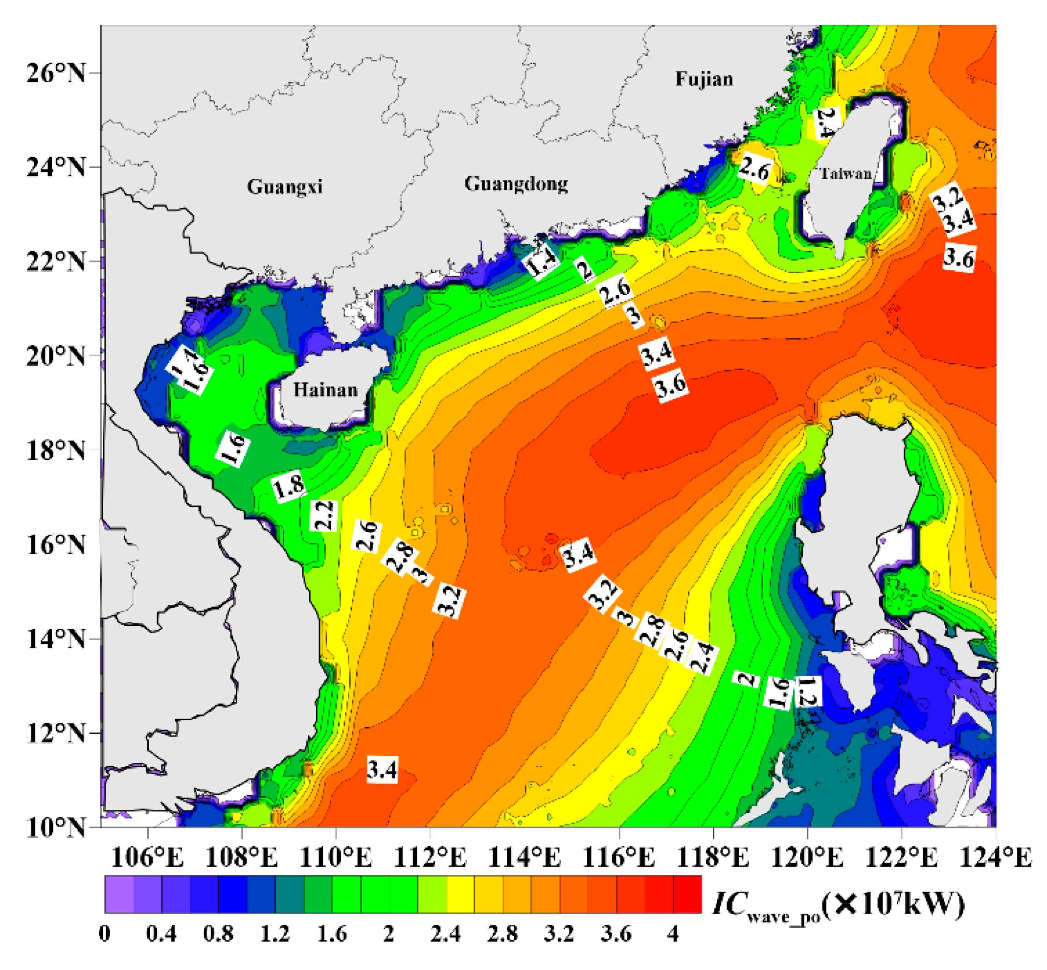
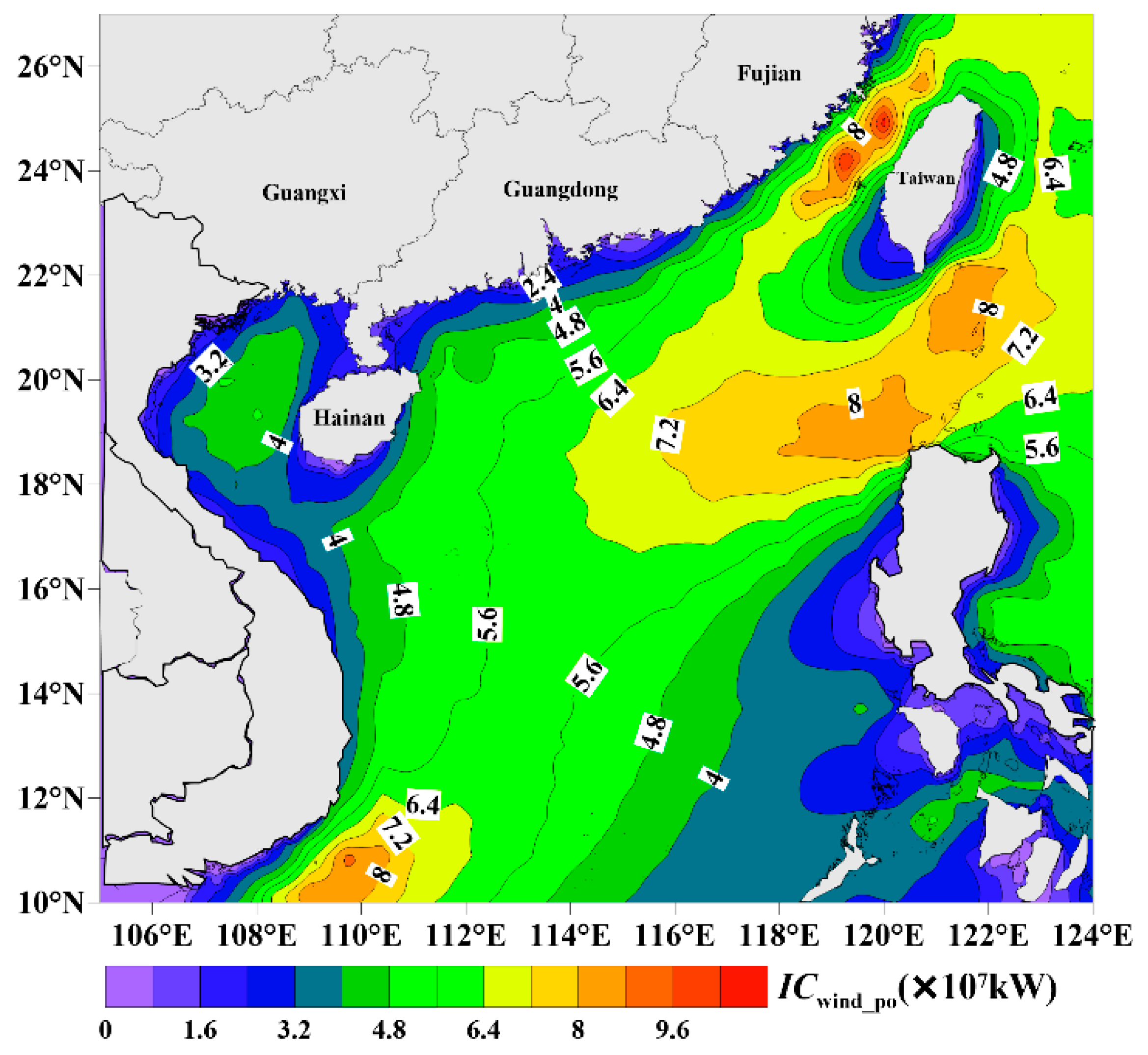
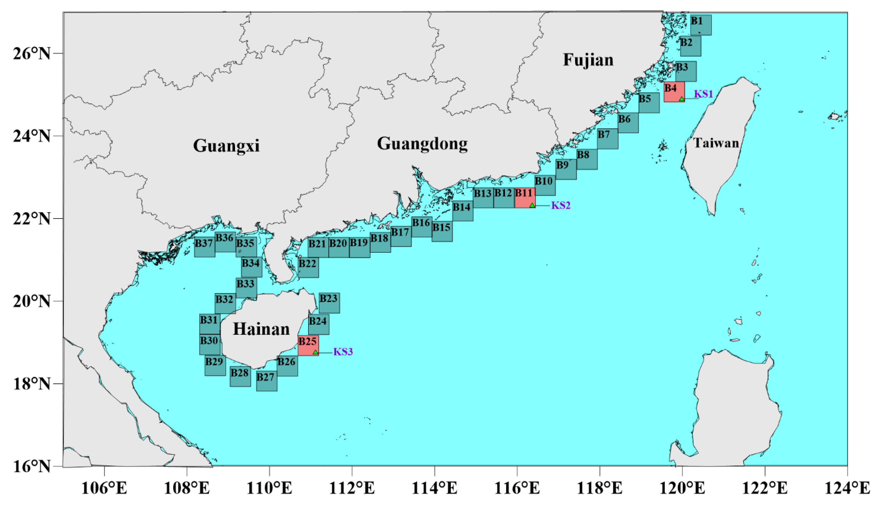
In nearshore waters of the South China Sea, 37 small areas with sizes of 0.5° × 0.5° were selected continuously and are shown in Figure 10. First, the annual average P_wy, annual average TE_wave, annual average IC_{wave_po}, annual average W, annual average TE_wind and annual average IC_{wind_po} of every grid were calculated for each small area, and the results for every grid in each small area were taken for averaging and were used as the annual average P_w, annual average TE_wave, annual average IC_{wave_po}, annual average W, annual average TE_wind and annual average IC_{wind_po} of each small area.

(2)

The joint quantitative division coefficient (JQDC) was defined as follows:

$$JQDC=(P_{\mathrm{wy}}·T{E}_{\mathrm{wave}}·I{C}_{\mathrm{wave}\_\mathrm{po}}) \times \left(W·T{E}_{\mathrm{wind}}·I{C}_{\mathrm{wind}\_\mathrm{po}}\right),$$

(7)

from which it can be seen that the potential of joint development increases with increasing JQDC.

(3)

According to JQDC, 5 grades were set. The criteria for the regional division in a general form are shown in

Table 4. Method used for regional division (general form)

Grade	Pwy (kW/m)	TEwave (h)	ICwave_po (× 107 kW)	W (W/m2)	TEwind (h)	ICwind_po (×107 kW)	JQDC	Suitability Level
1	<a1	<b1	<c1	<d1	<e1	<f1	<g1	poor
2	a1–a2	b1–b2	c1–c2	d1–d2	e1–e2	f1–f2	g1–g2	available
3	a2–a3	b2–b3	c2–c3	d2–d3	e2–e3	f2–f3	g2–g3	good
4	a3–a4	b3–b4	c3–c4	d3–d4	e3–e4	f3–f4	g3–g4	better
5	>a4	>b4	>c4	>d4	>e4	>f4	>g4	best

. From levels 1 to 5, the joint development potentials of wave and wind energy are increasing and are poor, available, good, better and best, respectively. For the range of each index in Table 4, there are different ranges of values for different areas. Threshold values a–g can be determined using the method in [31].

(4)

The criteria suitable for the nearshore waters of the South China Sea of regional division were established. The results are shown in

Table 5. Method of regional division used for nearshore waters of the South China Sea.

Grade	Pwy (kW/m)	TEwave (h)	ICwave_po (×107 kW)	W (W/m2)	TEwind (h)	ICwind_po (×107 kW)	JQDC (×1010)	Suitability Level
1	<2.62	<1919	<1.12	<180.58	<6809	<3.18	<2.20	poor
2	2.62–4.23	1919–2926	1.12–1.52	180.58–260.68	6809–7107	3.18–4.57	2.20–15.93	available
3	4.23–5.84	2926–3933	1.52–1.92	260.68–340.78	7107–7405	4.57–5.96	15.93–66.33	good
4	5.84–7.45	3933–4940	1.92–2.32	340.78–420.88	7405–7703	5.96–7.35	66.33–203.46	better
5	>7.45	>4940	>2.32	>420.88	>7703	>7.35	>203.46	best

.

According to the criteria of regional division established above, we calculated JQDC and undertook a regional division for 37 small areas with sizes of 0.5° × 0.5° in nearshore waters of the South China Sea. The results are shown in

Table 6. Regional division results.

Area	JQDC (×1010)	Grade	Area	JQDC (×1010)	Grade	Area	JQDC (×1010)	Grade
B1	32.36	3	B14	10.84	2	B27	12.32	2
B2	35.76	3	B15	22.62	3	B28	2.85	2
B3	120.24	4	B16	3.34	2	B29	6.26	2
B4	157.16	4	B17	2.58	2	B30	8.52	2
B5	56.18	3	B18	14.95	2	B31	8.17	2
B6	136.86	4	B19	25.12	3	B32	4.35	2
B7	18.53	3	B20	7.62	2	B33	0.16	1
B8	20.69	3	B21	4.72	2	B34	0.46	1
B9	28.44	3	B22	6.67	2	B35	0.47	1
B10	32.96	3	B23	55.21	3	B36	1.07	1
B11	95.16	4	B24	57.73	3	B37	3.14	2
B12	27.75	3	B25	72.49	4
B13	8.90	2	B26	33.22	3

. For this paper, 37 small areas were divided into four groups: the nearshore waters of Fujian Province (B1–B8), nearshore waters of Guangdong Province (B9–B22, B34), nearshore waters of Hainan Province (B23–B33), and nearshore waters of Guangxi Province (B35–B37). Because the nearshore waters of Guangxi are located in the Beibu Gulf, where the JQDC values are lower and the potential for development is also lower, that area was not included in this study. As shown in Table 6, in the other 3 groups, we selected 1 small area in each that could serve as the dominant areas for the various provinces’ nearshore waters to assess their wave and wind energy development potentials. The dominant area for Fujian nearshore waters is B4 (the grade of area B4 is four, and the JQDC is 157.16). The dominant area of Guangdong nearshore waters is B11 (the grade of area B11 is four, and the JQDC is 95.16). The dominant area of Hainan nearshore water is B25 (the grade of area B25 is four, and the JQDC is 72.49). The three dominant areas are shown in Figure 10 (red areas).

After determining the dominant areas, we selected key stations in the dominant areas. When selecting the key stations for the nearshore waters, we referred to the JQDC above and calculated the JQDC for every grid in the three dominant areas. The results are shown in

Table 7. The JQDC of each grid for the three dominant areas.

Longitude (° E)	Latitude (° N)	JQDC (×1010)	Longitude (° E)	Latitude (° N)	JQDC (×1010)	Longitude (° E)	Latitude (° N)	JQDC (×1010)
B4			B11			B25
119.625	24.875	117.13	116.000	22.250	119.72	110.750	18.750	64.07
119.750	24.875	153.97	116.125	22.250	128.79	110.875	18.750	72.67
119.875	24.875	201.91	116.250	22.250	139.73	111.000	18.750	79.10
120.000	24.875	348.24	116.375	22.250	151.76	111.125	18.750	86.30
119.625	25.000	104.94	116.000	22.375	87.98	110.750	18.875	62.02
119.750	25.000	142.35	116.125	22.375	99.57	110.875	18.875	70.49
119.875	25.000	191.20	116.250	22.375	112.04	111.000	18.875	76.71
120.000	25.000	328.51	116.375	22.375	126.43	111.125	18.875	84.08
119.625	25.125	73.67	116.000	22.500	---	110.750	19.000	60.31
119.750	25.125	90.10	116.125	22.500	---	110.875	19.000	68.57
119.875	25.125	234.27	116.250	22.500	89.90	111.000	19.000	75.01
120.000	25.125	208.21	116.375	22.500	105.06	111.125	19.000	82.38
119.625	25.250	79.73	116.000	22.625	---	110.750	19.125	59.09
119.750	25.250	81.04	116.125	22.625	---	110.875	19.125	67.32
119.875	25.250	203.63	116.250	22.625	---	111.000	19.125	73.71
120.000	25.250	170.94	116.375	22.625	---	111.125	19.125	81.10

and show that in each dominant area, the stations with the largest JQDC, which denote the highest development potentials, were selected as key stations. The information for the stations is shown in Figure 10 and Table 7. The three key stations are KS1 (120.000° E, 24.875° N), KS2 (116.375° E, 22.250° N), and KS3 (111.125° E, 18.750° N). In Table 7, “---” denotes that are no output wave data in this grid; therefore, when calculating the average values for each of the small areas, an average from the grids that included wave data outputs was calculated.

3.2.2. Wave Energy and Wind Energy Development Potential Assessment for the Key Stations

After determining the key stations for wave and wind energy development, indexes including annual average P_wy, annual average W, IC_{wave_po}, IC_{wind_po}, IC_{total_po}, the propagation direction of energy, the bivariate distributions of H_s-T_e for wave energy and the univariate distribution of ws for wind energy, the performance of well-known wave energy converters, and the economic efficiency and environmental efficiency of energy development were employed to assess wave and wind energy development potential in detail to provide valuable reference information for source development and utilization, converter design and operation.

(1) Overall Condition Analysis for Wave and Wind Energy

Based on 38 years of recent ERA-Interim data, indexes related to energy abundance were calculated for three key stations, and the results are shown in

Table 8. Results of wave and wind energy indexes at each key station.

Station	Longitude (° E)	Latitude (° N)	Water Depth (m)	Annual Average Pwy (kW/m)	Annual Average W (W/m2)	ICwave_po (×107 kW)	ICwind_po (×107 kW)	ICtotal_po (×107 kW)
KS1	120.000	24.875	54	6.09	620.89	2.45	10.84	13.29
KS2	116.375	22.250	52	9.08	294.65	2.41	5.25	7.66
KS3	111.125	18.750	144	8.44	243.50	2.31	4.44	6.75

. All annual average P_wy values exceeded 6.09 kW/m at the 3 key stations and were obviously higher than the criterion of exploitable wave energy (when P_w ≥ 2 kW/m, wave energy resources are usable) but did not reach the abundant level (when P_w ≥ 20 kW/m, wave energy resources are rich). 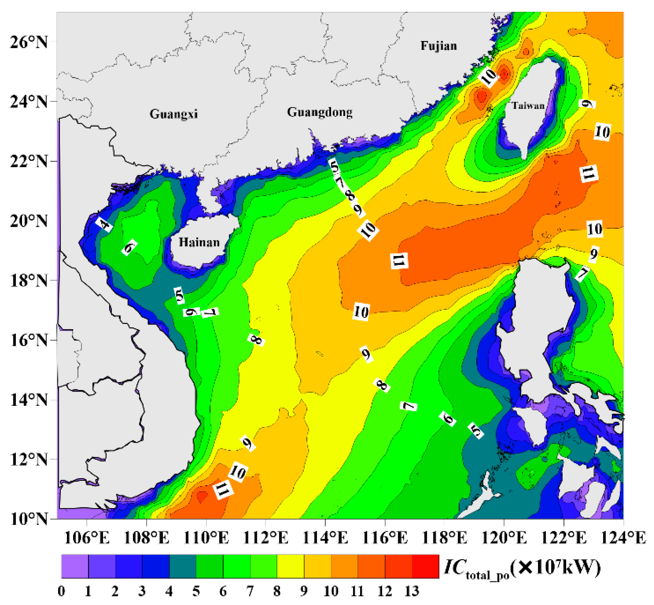The annual average W values all exceeded 243.50 W/m² for the three key stations and were higher than the criterion for the abundant level (when W ≥ 200 W/m², wind energy is rich) [18]. In addition, from the potential installed capacities, at the same station, the wind energy potential installed capacity exceeded the wave energy potential installed capacity, the total potential installed capacities all exceeded 6.75 × 10⁷ kW, and the total potential installed capacity for KS1 was the largest. Thus, the wave and wind energy development potentials are higher in the various nearshore dominant areas in the South China Sea.

(2) Wave and Wind Energy Propagation Directions

Research has shown that certain wave energy converters such as oscillating wave surge converters (OWSCs) have the highest absorbance efficiencies when the incident waves are orthogonal to the WECs [35]. Similarly, incident winds orthogonal to the windward sides of wind energy converters have the highest absorbance efficiencies. Therefore, we must study the propagation directions of wave and wind energy in different periods to adjust the directions of converters to acquire the largest amounts of energy. The propagation directions of wave and wind energy are important factors guiding operational converters. For this reason, in this study, we divided the period by season and calculated the percentages of the energy distributions in each direction, each season and for each key station and drew wave and wind power roses based on 38 years of recent ERA-Interim data.

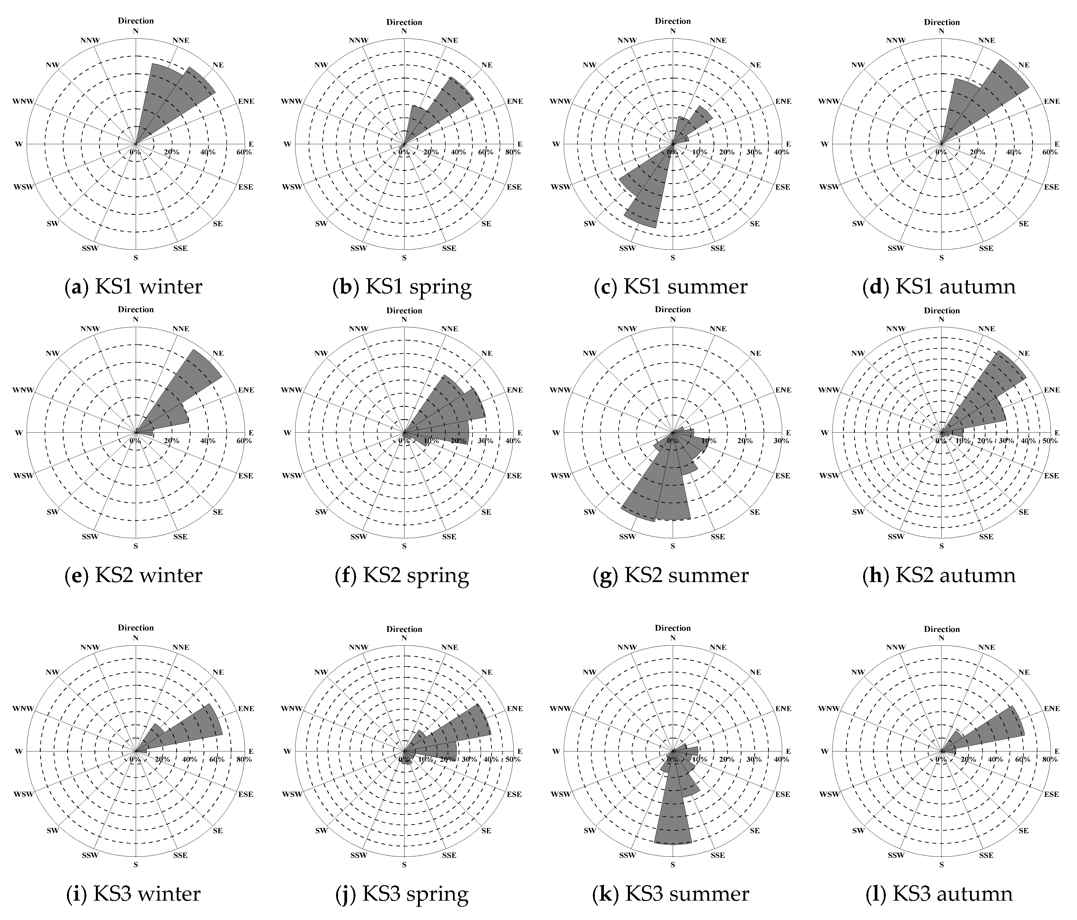
The results of wave power roses are shown in Figure 11. The results show that KS1 is located in the Taiwan Strait and is sheltered by land in its northwest and southeast directions, with an obvious narrowing effect. Therefore, as influenced by northeast and southwest monsoons, the propagation directions of wave energy in each season are mainly focused in the northeast and southwest directions. The dominant wave power directions were all NNE-NE (clockwise direction) in winter, spring and autumn, and the wave power accounted for approximately 99.5%, 91.1% and 95.8% of the total wave power, respectively. In summer, the direction of the dominant wave power was SSW-SW, and the wave power accounted for approximately 56.2% of the total wave power. KS2 is located in nearshore waters in the southeast of Guangdong and connects with the West Pacific in the east via the Luzon Strait; this location will be influenced by monsoons and typhoons from the West Pacific in each season. Compared with KS1, the direction of the wave energy rotated eastward in winter, spring and autumn, the direction of the dominant wave power was all NE-E, and the wave power accounted for approximately 96.1%, 80.4% and 86.7% of the total wave power, respectively. In summer, the direction of the dominant wave power was SSE-SSW and the wave power accounted for approximately 63.0% of the total wave power. When influenced by typhoons, incident wave energy was strongly enhanced in the E and SE directions in spring and summer. KS3 is located in nearshore waters east of Hainan, and under the influence of topography, the direction of the wave energy continuously rotated eastward in winter, spring and autumn, the direction of the dominant wave power was NE-E and predominantly ENE, and the wave power accounted for approximately 98.2%, 76.6% and 91.3% of the total wave power, respectively. In summer, the direction of the dominant wave power was SSE-S and the wave power accounted for approximately 53.3% of the total wave power. The results show that wave energy was more concentrated in winter, spring and autumn, which is beneficial for the highest energy absorption.

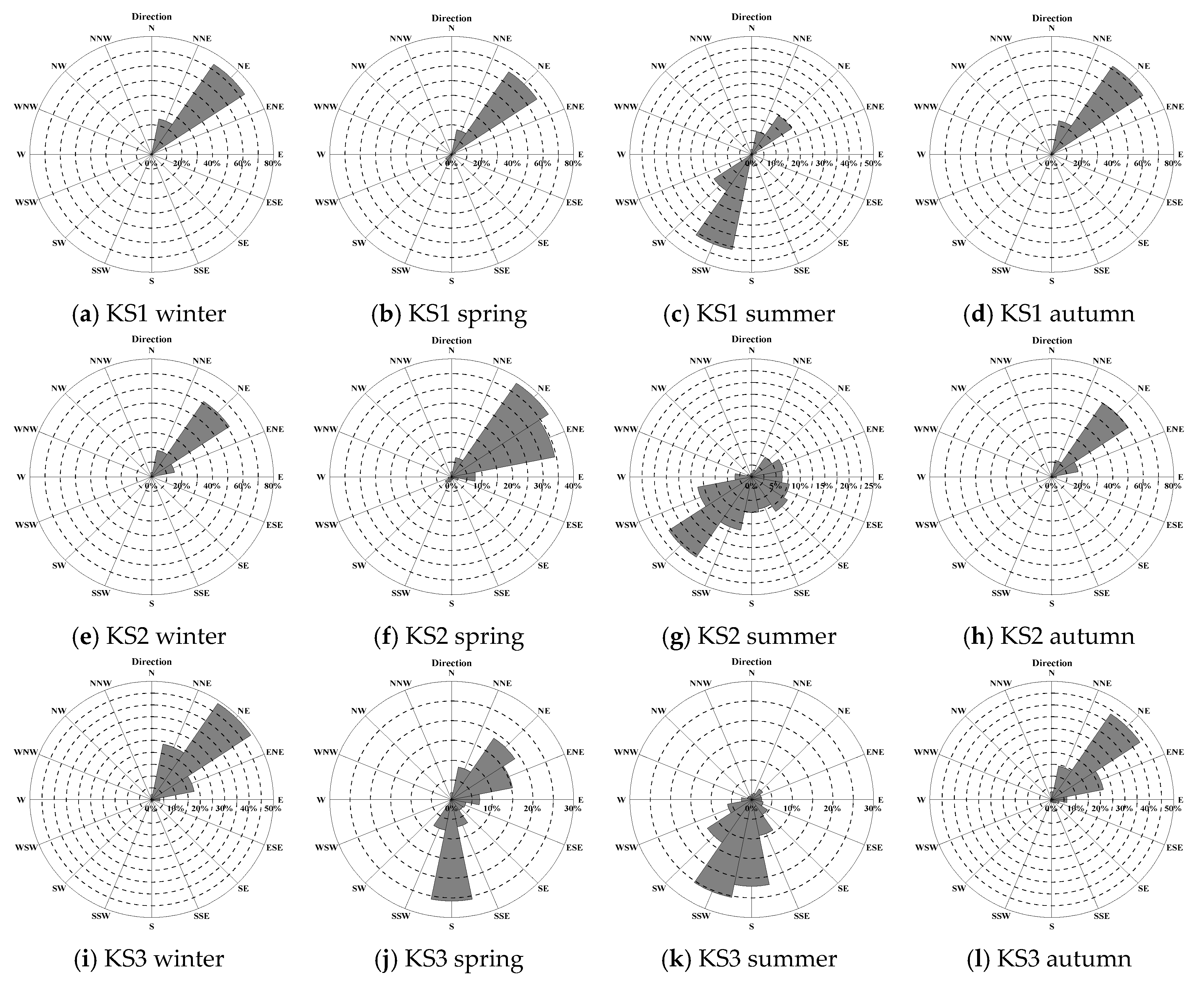
The results of wind power roses are shown in Figure 12. Regarding the wind energy for KS1, the direction of the dominant wind power was also always NNE-NE in winter, spring and autumn, and the wind power accounted for approximately 97.8%, 84.2% and 95.1% of the total wind power, respectively. However, compared with wave energy, the percentage of wind energy was strongly enhanced in the NE direction, which was caused by northeast monsoons in those three seasons. In summer, the direction of the dominant wind power was SSW-SW and the wind power accounted for approximately 59.7% of the total wind power. The results show that wind energy was also more concentrated in winter, spring and autumn, which benefits wind energy development. Regarding the wind energy in KS2, the direction of the dominant wind power was NE-ENE in winter, spring and autumn, and the wind power accounted for approximately 76.7%, 72.6% and 77.9% of the total wind power, respectively. In summer, the direction of the dominant wind power was SSW-WSW and the wind power accounted for approximately 43.3% of the total wind power. The regularities of the distribution and cause were similar to those for the wave energy direction distribution. Regarding the wind energy at KS3, the direction of the dominant wind power was mainly NNE-ENE in winter and autumn, and the wind power accounted for approximately 90.5% and 79.5% of the total wind power, respectively, which reflected the influence northeast monsoons. There was a transition between northeast and southwest monsoons in spring such that there were two dominant wind power directions, NNE-ENE and SSE-SSW, and the wind power accounted for approximately 42.4% and 40.8% of the total wind power, respectively. In summer, the direction of the dominant wind power was S-SW and the wind power accounted for approximately 60.5% of the total wind power.

In conclusion, the wave and wind energy propagation directionality was better for the nearshore key stations in various seasons in the South China Sea. In each season, the propagation direction was fixed, which is advantageous for adjusting the directions of wave and wind energy converters. The results can provide important references for mooring wave and wind energy converters in various seasons.

(3) Bivariate Distributions of H_s-T_e for Wave Energy and Univariate Distributions of ws for Wind Energy

Bivariate distributions of H_s-T_e for wave energy can serve as an important index for wave energy assessments that can be used to determine dominant wave condition, which makes a dominant contribution to total wave energy density and can be an important index for wave energy converter (WEC) design. In addition, this index is a basic parameter for assessing the power generation performance of WECs, which can be represented with a scatter diagram [36]. Referring to the above index, the univariate distribution of ws for wind energy can also be an important index for wind energy assessments that can be used to determine dominant wind conditions that make a dominant contribution to total wind energy density and can be an important index for wind energy converter design.

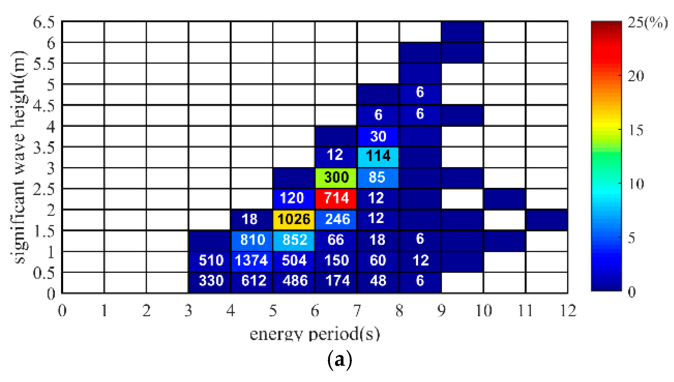
In order to grasp bivariate distributions of H_s-T_e for wave energy in each key station, based on the ERA-Interim data over the last 38 years, using an H_s interval of 0.5 m and a T_e interval of 1 s, we calculated the percentage of the total wave energy density (the mean of the sum of P_w multiplied by the number of hours in a year in MWh/(m·year)) under each wave condition to the total wave energy density under all wave conditions [25,31]; the results are shown in Figure 13. In the figure, the color code denotes the percentage and the numbers denote the annual average total number of hours for which particular sea states occurred each year. The results show that the dominant wave condition at station KS1 had H_s values of 0–3.5 m and T_e values of 4–8 s and the wave energy accounted for 92.79% of the total wave energy density. At station KS2, the dominant wave condition had H_s values of 0.5–3.5 m and T_e values of 5–9 s and the wave energy accounted for 87.60% of the total wave energy density. At station KS3, the dominant wave condition had H_s values of 0.5–3.5 m and T_e values of 4–9 s and the wave energy accounted for 87.35% of the total wave energy density. The dominant wave conditions in the key nearshore stations in the South China Sea were the same and thus can serve as an important basis for the design of effective wave conditions of WECs.

In addition, the number of hours can help us understand the occurrence of particular wave condition each year which is meaningful for the design of WECs. The results show that the number of hours under a wave condition with an H_s value of 0.5–1.0 m and a T_e value of 4–5 s at station KS1 was the highest at 1374 h. The number of hours at a wave condition with an H_s value of 0.5–1.0 m and a T_e value of 6–7 s at station KS2 was the highest at 1104 h, and the number of hours at a wave condition with an H_s value of 0.5–1.0 m and a T_e value of 5–6 s at station KS3 was the highest at 1362 h. Regarding the wave conditions at each key station, the H_s values were all 0.5–1.0 m for the majority of hours. However, the ratio of the wave energy under the most common wave conditions to the total wave energy density was not the highest. At stations KS1 and KS2, the wave conditions with the highest ratio of the total wave energy density were an H_s value of 2.0–2.5 m and a T_e value of 6–7 s. At station KS3, the wave conditions with the highest ratio of the total wave energy density were an H_s value of 2.0–2.5 m and a T_e value of 7–8 s. The annual average number of hours under those wave conditions were 714, 612 and 456 h for stations KS1, KS2 and KS3, respectively. From the above results, number of hours of optimal wave conditions was not necessarily related to the contribution to total energy.

The bivariate distributions of H_s-T_e for wave energy have important meaning for wave energy development and utilization. Rusu and Soares have indicated that actual wave power yield depends on the particular WEC device as rated by its wave power generation because each technology has different operational ranges and different efficiencies under various sea states [37]. Contestabile et al. constructed an optimal configuration assessment in terms of the financial returns of the Overtopping BReakwater for wave Energy Conversion (OBREC) [38]. Vannucchi and Cappietti assessed the performances of 6 state-of-the art WECs in Italian nearshore waters [39]. Silva et al. evaluated the feasibility of different wave energy converting technologies in Portugal’s nearshore waters [36]. Rusu assessed wave energy conversion efficiency in various coastal environments [40]. For the present paper, we employed well-known WECs that were used in the past for similar studies and are well accepted among academics to find suitable WECs for the nearshore waters of the South China Sea. Additionally, the electricity generation performance of well-known WECs in the three key stations in the nearshore waters of the South China Sea were evaluated. Considering the water depths all exceed 50 m, we selected 3 WECs that are suitable for 50 m and greater water depths: AquaBuoy (>50 m) [41], AWS (>50 m) [42] and Pelamis (>50 m) [43]. Indexes including mean power output (P_e, kW), capacity factor (C_f, %) and relative capture width (R_cw, %) were employed to evaluate the performances of the WECs. The calculation methods are as follows [31,39]:

$$P_{\mathrm{e}}={\sum }_{\mathrm{i}=1}^{\mathrm{nT}}{\sum }_{\mathrm{j}=1}^{\mathrm{nH}}{P}_{\mathrm{ij}} \times f_{\mathrm{ij}},$$

(8)

$$C_{\mathrm{f}}=\frac{P_{\mathrm{e}}}{\mathrm{Rated} \mathrm{power}}, \mathrm{and}$$

(9)

$$R_{\mathrm{cw}}=\frac{C_{\mathrm{w}}}{main\_\dim ension},$$

(10)

where nT is the number of T_e classes, and nH is the number of H_s classes. P_ij is the power output of the device, which originates from the power matrix for the specific WEC. The power matrices were collected from the open literature [36,44]. f_ij is the occurrence frequency for various sea states, which was collected from scatter diagrams shown in Section 3.2.2 (3). The rated powers (units: kW) are the rated powers of the WECs. The rated powers of the different WECs were 250 kW (AquaBuoy), 2000 kW (AWS), and 750 kW (Pelamis). C_w is capture width (m) and can be calculated by:

$$C_{\mathrm{w}}=\frac{P_{\mathrm{e}}}{P_{\mathrm{wy}}}.$$

(11)

main_dim ension is the main dimension of a WEC. The main dimension of AquaBuoy is 20 m [41], that for AWS is 144 m [45], and that for Pelamis is 180 m [46].

According to the method above and the ERA-Interim wave field data from 1979–2016, we calculated the mean power output, capacity factor and relative capture width. The results are shown in

Table 9. Mean power outputs, capacity factors and relative capture widths for the key stations.

Location	Mean Power Output “Pe” (kW)			Capacity Factor “Cf” (%)			Relative Capture Width “Rcw” (%)
	AB	AWS	Pelamis	AB	AWS	Pelamis	AB	AWS	Pelamis
KS1	9.87	19.45	36.60	3.95	0.97	4.88	8.11	2.22	3.34
KS2	17.03	44.20	60.08	6.81	2.21	8.01	9.38	3.38	3.68
KS3	16.32	46.76	54.20	6.53	2.34	7.23	9.67	3.85	3.57

. From the results, for the 3 key stations, P_e and C_f were the highest when using the Pelamis WEC, and the Pelamis WEC apparently is the best suited WEC when considering these two indexes. However, when considering R_cw, AquaBuoy apparently is the best suited WEC because R_cw was highest when it was used. The main reason for this result is that AquaBuoy’s dimensions are relatively small, differing by an order of magnitude from those of the AWS and Pelamis WECs. In addition, from the C_f results, even for the Pelamis, which had the highest conversion efficiency, the C_f values for the 3 key stations were no greater than 10%. The conversion efficiency was still lower. The results show that the well-known WECs were not suitable for wave energy development in the nearshore of the South China Sea. We must consider the distributions of wave conditions in the area of interest and design power matrix for WECs and develop more suitable WECs for this area to improve conversion efficiency. This work will be carried out in our future work.

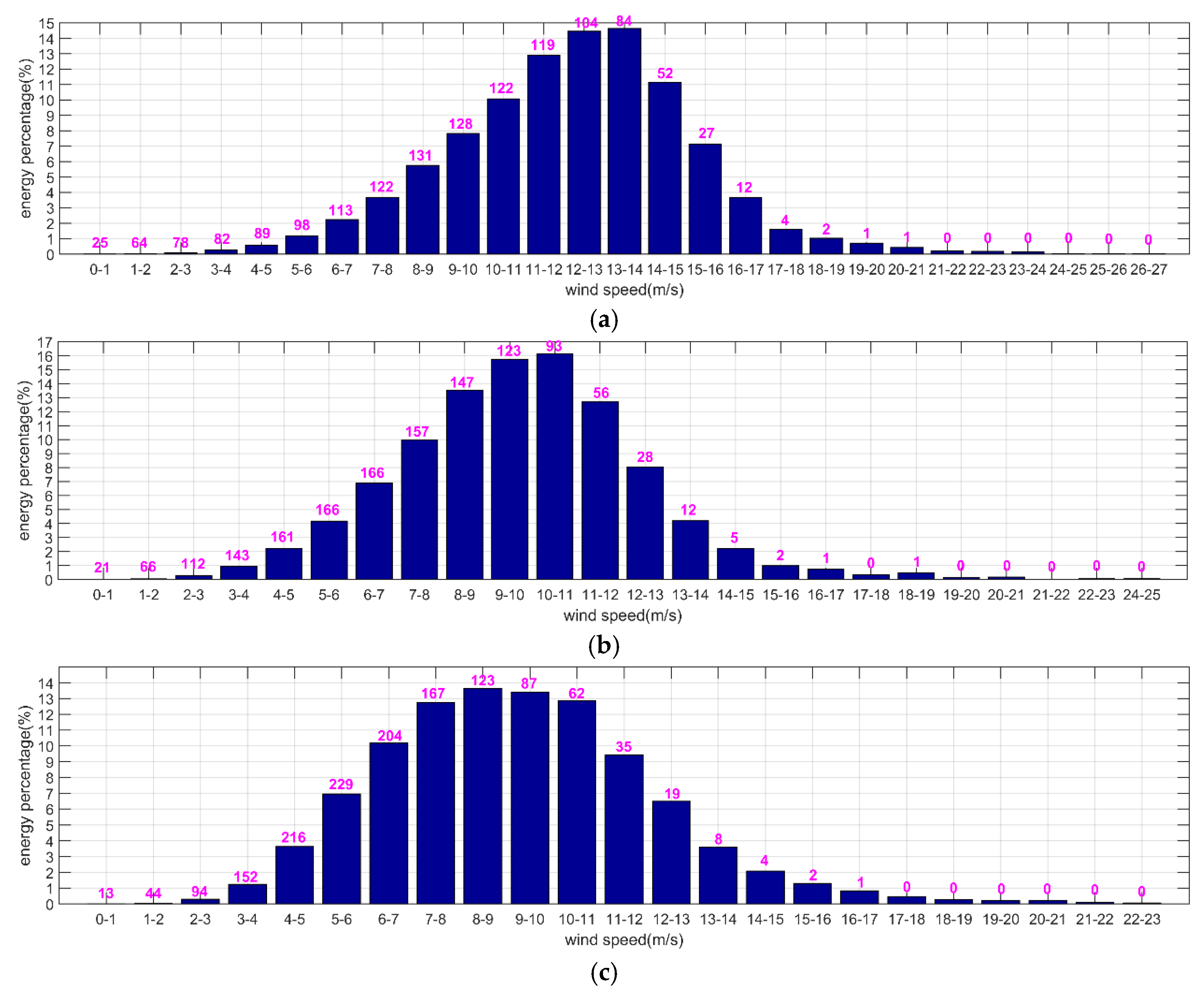
Based on the ERA-Interim data over the last 38 years and using a ws interval of 1 m/s, we calculated the percentage of the total wind power density (the mean of the sum of W multiplied by the number of hours in a year kWh/(m²·year)) under each wind speed to the total wind power density under all wind speeds; the results are shown in Figure 14. In the figure, the horizontal axis denotes the range of wind conditions, the vertical axis denotes the percentage of energy, and the number denotes the annual average number of times under each wind condition. The results show that the dominant wind condition at station KS1 had ws values of 6–17 m/s, and the wind energy accounted for 93.49% of the total wind energy density. At station KS2, the dominant wind condition had ws values of 4–15 m/s and the wind energy accounted for 95.75% of the total wind energy density. At station KS3, the dominant wind condition had ws values of 4–15 m/s and the wind energy accounted for 94.98% of the total wind energy density. At each key station, wind energy was concentrated in the ws range of 4–17 m/s. Wind energy was scarce for low wind speeds of ws < 4 m/s and for high wind speeds of ws > 17 m/s.

In addition, the number of occurrences of wind conditions can help us understand the occurrence of particular wind condition each year which is meaningful for the design of wind energy converters. The results show that the number of occurrences of wind conditions with ws values of 8–9 m/s at station KS1 was the highest, at 131, but the ratio of the wind energy under the most common wind conditions to the total wind energy density was not the highest. The wind condition with the highest ratio of the total wind energy density was that with a ws value of 13–14 m/s, for which the annual average number of occurrences was 84. The number of occurrences of wind conditions with ws values of 5–6 m/s and 6–7 m/s at station KS2 was the highest, at 166, but the ratio of the wind energy under the most common wind conditions to the total wind energy density was also not the highest. The wind condition with the highest ratio of the total wind energy density was that with a ws value of 10–11 m/s, and the annual average number of occurrences was 93. The number of occurrences of a wind condition with a ws value of 5–6 m/s at station KS3 was the highest, at 229, but the ratio of the wind energy under the most common wind conditions to the total wind energy density was also not the highest. The wind condition with the highest ratio of the total wind energy density was that with a ws value of 8–9 m/s, and the annual average number of occurrences was 123. According to the above results, the number of occurrences of wind condition was not necessarily related to the contribution to total energy. At each key station, the medium wind speed provided the maximum contribution to the total wind energy density, and the number of occurrences of medium wind speeds was also maximum. Therefore, wind energy in the nearshore South China Sea is mainly provided by winds of medium wind speeds.

(4) Economic Benefit and Environmental Benefit Assessment for Wave and Wind Energy Development

When assessing wave and wind energy potential, except for energy distribution, we must also assess the economic and environmental benefits of energy development to provide useful information for project decision makers. Regarding economic benefit, in the wave energy section, the annual average generated energy per km of wavefront length (E_{wave_mean}, unit: kWh/km/a) was employed, calculated by:

$$E_{\mathrm{wave}\_\mathrm{mean}}=P_{wy} \times 8760h \times 1 \mathrm{km},$$

(12)

and in the wind energy section, the annual average generated energy per km² area (E_{wind_mean}, units: kWh/km²/a) was employed, calculated by:

$$E_{\mathrm{wind}\_\mathrm{mean}}=W \times 8760h \times 1{ \mathrm{km}}^2,$$

(13)

where E_{wave_mean} and E_{wind_mean} are the theoretically produced energies in a specific length and area. However, Contestabile et al. indicated that economic and environmental analyses, generally speaking, should refer to real produced energy and not to theoretically produced energy. This potential produced energy takes into account wave-to-wire efficiency or wind-to-wire efficiency [47]. Therefore, in this paper, we considered an average efficiency of the three WECs and an average efficiency of the wind generator and calculated the potential produced energy for wave energy (E_{wec_mean}, unit: kWh/km/a) and wind energy (E_{turb_mean}, unit: kWh/km²/a). For a generic WEC, the overall averaged efficiency was 16.5%, and the maximum energy derived from a wind generator was only 59% of the available wind kinetic energy [47]. Based on 38 years of recent ERA-Interim data, the theoretically produced energy and the potential produced energy for wave and wind energy were calculated for the 3 key stations. The potential produced energy was then converted to saved total raw coal quantity (unit: ton/a) to reflect the economic benefits for wave and wind energy development. The reduced total carbon dioxide (unit: ton/a) was calculated after developing the wave energy from the annual average per km of wavefront length and the wind energy from the annual average per km² of area to reflect the environmental benefit from wave and wind energy development. Each index is shown in

Table 10. Economic benefit and environment benefit indexes at each key station.

Station	Ewave_mean (kWh/km/a)	Ewec_mean (kWh/km/a)	Ewind_mean (kWh/km2/a)	Eturb_mean (kWh/km2/a)	Saved Total Raw Coal Quantity (ton/a)	Reduced Total Carbon Dioxide (ton/a)
KS1	53,348,400	8,802,486	5,438,996,400	3,209,007,876	395,469	1,028,219
KS2	79,540,800	13,124,232	2,581,134,000	1,522,869,060	188,773	490,810
KS3	73,934,400	12,199,176	2,133,060,000	1,258,505,400	156,170	406,042

Note: 1 kWh of generated energy requires 0.1229 kg of raw coal, and 1 ton of raw coal will generate 2.6 tons of carbon dioxide.

.

The results show that the economic and environmental benefits from the joint development of wave and wind energy were higher at key stations in the nearshore South China Sea. For the small areas of each key station, the annual average joint potential produced energies that all exceeded 12.7 × 10⁸ kWh and the generating capacities were higher. Wave energy and wind energy can provide stable energy supplies for coastal cities, islands and oil platforms, for example. The economic benefit is remarkable. In addition, the annual average saved total raw coal quantity exceeded 150,000 tons, and the reduced total carbon dioxide exceeded 400,000 tons. The environmental benefit is also remarkable.

4. Discussion

In Section 3.1, we analyzed in detail the joint development potential of offshore wave and wind energy in the South China Sea. The results showed that the areas with relatively high annual average wave power densities (approximately 14–17 kW/m) are primarily located in the western sea area of the Luzon Strait in the central South China Sea and the southeastern sea area of Taiwan. From a worldwide perspective, wave energy is not abundant in the South China Sea, but within the China Sea, the wave energy in the South China Sea is most abundant in various areas. In addition, the seasonal variation in wave power density is considerable, and winter and autumn are the key development periods because of monsoons and typhoons.

Regarding wind energy, there are three areas of large wind power density values in the Taiwan Strait (450 W/m²), Luzon Strait (400–450 W/m²), and southeastern sea areas of the Indo-China Peninsula (350–450 W/m²). The reasons for the large values pertain to monsoons and typhoons. Similar to wave energy, the seasonal variation in wind power density is obvious, and winter and autumn are the key development periods for wind energy development.

In this paper, we present a new index, potential installed capacity, for wave and wind energy assessment that can aid in assessments of wave and wind energy using a uniform unit (×10⁷ kW) in the future. By using joint potential installed capacity, we determined that there are three highly promising areas for the development of wave and wind energy: the Taiwan Strait (10 × 10⁷ kW), the Luzon Strait (10 × 10⁷ kW–11 × 10⁷ kW) and the southeastern sea area of the Indo-China Peninsula (9 × 10⁷ kW–11 × 10⁷ kW).

In Section 3.2, we analyzed in detail the joint development potential of wave and wind energy in the nearshore area of the South China Sea. The results showed that the dominant areas in nearshore waters were areas B4, B11 and B25, which are located in Fujian nearshore waters, Guangdong nearshore waters and Hainan nearshore waters, respectively. Three key stations (KS1, KS2, and KS3), one each from the three dominant areas, were then selected. In selecting the dominant areas and key stations, JQDC, which is based on only the richness level of wave and wind energy, was established and used. In addition to richness level, we must consider other factors such as water depth, which is a critical consideration when planning offshore wind or wave energy farms. Certain well-known WECs such as AquaBuoy (>50 m), AWS (>50 m), Pelamis (>50 m), Oyster (15 m) and Wave Star (Nearshore) can be used at specific water depths in relatively nearshore waters. For selected key stations KS1, KS2 and KS3, the water depths are 54 m, 52 m and 144 m, respectively. Therefore, from the perspective of WECs, the water depths of the three key stations are suitable for siting wave and wind energy farms. In addition, considering the cost of the construction and maintenance of wave and wind energy farms, shallow water depth areas will possibly be suitable locations for wave and wind energy farms. From that perspective, areas B4, B11 and B25, which have water depths of 150 m or less, are suitable areas.

At the key stations, in each season, the propagation direction was fixed, which is advantageous for adjusting the directions of wave energy converters and wind energy converters. In winter, spring and autumn, the direction of the dominant wave power was NNE-NE; in summer, the direction of the dominant wave power was SSW-SW. In winter, spring and autumn, the direction of the dominant wind power was also NNE-NE, and in summer, the direction of the dominant wind power was SSW-SW. The dominant wave conditions all had H_s values of 0–3.5 m and T_e values of 4–9 s, and the wave energy accounted for 89% of the total wave energy density, which can be a uniform standard for the design of new WECs that are suitable for these local areas. At each key station, wind energy was concentrated in the ws range of 4–17 m/s. Wind energy was scarce for low wind speeds of ws < 4 m/s and for high wind speeds of ws > 17 m/s. Wind energy in the nearshore South China Sea is mainly provided by winds with medium speeds. At present, there are no suitable and well-known WECs for cost-efficient wave energy conversion at the three key stations in the nearshore waters of the South China Sea. Considering the average efficiencies of the WECs and wind generators, the economic and environmental benefits for the joint development for wave and wind energy were relatively higher for the key stations in the nearshore South China Sea. The joint development potential of wave and wind energy is higher in the South China Sea.

5. Conclusions

Based on 38 years of recent high-resolution and high-accuracy ERA-Interim reanalysis wave and wind field data, the temporal and spatial distributions and the joint development potentials for wave and wind energy were studied in detail in offshore and nearshore (key stations) waters of the South China Sea. The following conclusions can be put forth:

(1)

In the South China Sea, wave and wind energy is abundant. The relatively abundant areas of wave energy are located in the western area of the Luzon Strait in the central South China Sea and the southeastern sea area of Taiwan. The relatively abundant areas of wind energy are located in the Taiwan Strait, the Luzon Strait and the southeastern sea area of the Indo-China Peninsula. The wave and wind energy distribution trends differed somewhat. The potential installed capacity presented in this paper will allow us to assess wave and wind energy using a uniform standard. From the distributions of wave and wind energy joint potential installed capacity, joint development dominant areas for wave and wind energy were still found to be located in the Taiwan Strait, the Luzon Strait and the southeastern sea area of the Indo-China Peninsula. The above results will provide important references for decision makers concerned with the joint development of wave and wind energy projects.

(2)

In the nearshore of the South China Sea, there are three dominant areas of joint development potential for wave and wind energy: the southeastern nearshore waters of Fujian Province (B4 area), the southeastern nearshore waters of Guangdong Province (B11 area) and the southeastern nearshore waters of Hainan Province (B25 area). For the key stations of these areas, including KS1, KS2 and KS3, the wave and wind energy development potentials are all higher. At the key stations, the propagation directions of wave energy in various seasons are basically consistent, and the directionalities are better, which is advantageous to wave energy development. The directionality of wind energy was found to be similar to that of wave energy. The results can provide important references for mooring wave energy converters and wind energy converters in various seasons. At key stations, the dominant wave and dominant wind conditions were the same and can act as important references for designing and operating wave and wind energy converters to improve the use ratios of wave and wind energy. Pelamis appears to be the WEC best suited to the dominant areas, but its conversion efficiency is still lower, and it is not suitable for wave energy development in the areas of interest. Therefore, we must consider wave condition distributions and develop more suitable WECs for the areas of interest.

(3)

The economic and environment benefits of the joint development of wave and wind energy are high. By jointly developing wave and wind energy, the hardware facilities of power plants will be better utilized, the quantities of energy output will be improved, and the costs of energy transfer will be reduced. The joint development of wave and wind energy is a promising trend for ocean renewable energy development. In this paper, we explored only the joint development potential of wave and wind energy in the South China Sea to provide definite references for joint energy development.

References

1. Cornett, A.M. A global wave energy resource assessment. In Proceedings of the 18th International Conference on Offshore and Polar Engineering, Vancouver, BC, Canada, 6–11 July 2008. [Google Scholar]
2. Arinaga, R.A.; Cheung, K.F. Atlas of global wave energy from 10 years of reanalysis and hindcast data. Renew. Energy 2012, 39, 49–64. [Google Scholar] [CrossRef]
3. Zheng, C.W.; Shao, L.T.; Shi, W.L.; Su, Q.; Lin, G.; Li, X.Q.; Chen, X.B. An assessment of global ocean wave energy resources over the last 45 a. Acta Oceanol. Sin. 2014, 33, 92–101. [Google Scholar] [CrossRef]
4. Zheng, C.W.; Pan, J. Assessment of the global ocean wind energy resource. Renew. Sustain. Energy Rev. 2014, 33, 382–391. [Google Scholar] [CrossRef]
5. Zheng, C.W.; Li, C.Y.; Pan, J.; Liu, M.Y.; Xia, L.L. An overview of global ocean wind energy resource evaluations. Renew. Sustain. Energy Rev. 2016, 53, 1240–1251. [Google Scholar] [CrossRef]
6. Zheng, C.W.; Wang, Q.; Li, C.Y. An overview of medium- to long-term predictions of global wave energy resources. Renew. Sustain. Energy Rev. 2017, 79, 1492–1502. [Google Scholar] [CrossRef]
7. Iglesias, G.; Carballo, R. Wave energy potential along the Death Coast (Spain). Energy 2009, 34, 1963–1975. [Google Scholar] [CrossRef]
8. Iglesias, G.; Lopez, M.; Carballo, R.; Castro, A.; Fraguela, J.A.; Frigaard, P. Wave energy potential in Galicia (NW Spain). Renew. Energy 2009, 34, 2323–2333. [Google Scholar] [CrossRef]
9. Iglesias, G.; Carballo, R. Offshore and inshore wave energy assessment: Asturias (N Spain). Energy 2010, 35, 1964–1972. [Google Scholar] [CrossRef]
10. Iglesias, G.; Carballo, R. Wave energy resource in the Estaca de Bares area (Spain). Renew. Energy 2010, 35, 1574–1584. [Google Scholar] [CrossRef]
11. Iglesias, G.; Carballo, R. Wave power for La Isla Bonita. Energy 2011, 35, 5013–5021. [Google Scholar] [CrossRef]
12. Iglesias, G.; Carballo, R. Choosing the site for the first wave farm in a region: A case study in the Galician Southwest (Spain). Energy 2011, 36, 5525–5531. [Google Scholar] [CrossRef]
13. Kim, G.; Jeoug, W.M.; Lee, K.S.; Jun, K.; Lee, M.E. Offshore and nearshore wave energy assessment around the Korean Peninsula. Energy 2011, 36, 1460–1469. [Google Scholar] [CrossRef]
14. Yamaguchi, A.; Ishihara, T. Assessment of offshore wind energy potential using mesoscale model and geographic information system. Renew. Energy 2014, 69, 506–515. [Google Scholar] [CrossRef]
15. Ko, D.H.; Jeong, S.T.; Kim, Y.C. Assessment of wind energy for small-scale wind power in Chuuk State, Micronesia. Renew. Sustain. Energy Rev. 2015, 52, 613–622. [Google Scholar] [CrossRef]
16. Fang, H.F. Wind energy potential assessment for the offshore areas of Taiwan west coast and Penghu Archipelago. Renew. Energy 2014, 67, 237–241. [Google Scholar] [CrossRef]
17. Rusu, E.; Onea, F. Evaluation of the wind and wave energy along the Caspian Sea. Energy 2013, 50, 1–14. [Google Scholar] [CrossRef]
18. Zheng, C.W.; Pan, J.; Li, J.X. Assessing the China Sea wind energy and wave energy resources from 1988 to 2009. Ocean Eng. 2013, 65, 39–48. [Google Scholar] [CrossRef]
19. Zheng, C.W.; Zhuang, H.; Li, X.; Li, X.Q. Wind energy and wave energy resources assessment in the East China Sea and South China Sea. Sci. China Technol. Sci. 2012, 55, 163–173. [Google Scholar] [CrossRef]
20. Zheng, C.W.; Lin, G.; Shao, L.T. Wave energy resources analysis around Taiwan waters. J. Nat. Resour. 2013, 28, 1179–1186. [Google Scholar]
21. Liang, B.C.; Fan, F.; Liu, F.S.; Gao, S.H.; Zuo, H.Y. 22-Year wave energy hindcast for the China East Adjacent Seas. Renew. Energy 2014, 71, 200–207. [Google Scholar] [CrossRef]
22. Anoop, T.R.; Kumar, V.S.; Shannas, P.R.; Johnson, G. Surface wave climatology and its variability in the North Indian Ocean based on ERA-Interim reanalysis. J. Atmos. Ocean. Technol. 2015, 32, 1372–1385. [Google Scholar] [CrossRef]
23. Semedo, A.; Suselj, K.; Rutgersson, A.; Sterl, A. A global view on the wind sea and swell climate and variability from ERA-40. J. Clim. 2011, 24, 1461–1479. [Google Scholar] [CrossRef]
24. Shanas, P.R.; Kumar, V.S. Trends in surface wind speed and significant wave height as revealed by ERA-Interim wind wave hindcast in the Central Bay of Bengal. Int. J. Climatol. 2015, 35, 2654–2663. [Google Scholar] [CrossRef]
25. Wan, Y.; Zhang, J.; Meng, J.M.; Wang, J. Wave energy assessment in the East China Sea and South China Sea based on ERA-Interim high resolution data. Acta Energ. Sol. Sin. 2015, 36, 1259–1267. [Google Scholar]
26. Wan, Y.; Zhang, J.; Meng, J.M.; Wang, J. Exploitable wave energy assessment based on ERA-Interim reanalysis data—A case study in the East China Sea and the South China Sea. Acta Oceanol. Sin. 2015, 34, 143–155. [Google Scholar] [CrossRef]
27. Wu, L.L.; Wang, X.L.; Feng, Y. Historical wave height trends in the South and East China Seas, 1911–2010. J. Geophys. Res. Oceans 2014, 119, 4399–4409. [Google Scholar] [CrossRef]
28. Zhou, L.; Zheng, C.W.; Li, J.; Chen, X.B. Wave energy research in global oceans with ERA-40 wave data for recent 45 years. In Proceedings of the 2011 International Conference on Remote Sensing, Environment and Transportation Engineering (RSETE), Nanjing, China, 24–26 June 2011. [Google Scholar]
29. Zheng, C.W.; Jia, B.K.; Guo, S.P.; Zhuang, H. Wave energy resource storage assessment in global ocean. Resour. Sci. 2013, 35, 1611–1616. [Google Scholar]
30. Pontes, M.T. Assessing the European wave energy resource. J. Offshore Mech. Arct. Eng. 1998, 120, 226–231. [Google Scholar] [CrossRef]
31. Wan, Y.; Fan, C.Q.; Zhang, J.; Meng, J.M.; Dai, Y.S.; Li, L.G.; Sun, W.F.; Zhou, P.; Wang, J.; Zhang, X.D. Wave energy resource assessment off the coast of China around the Zhoushan Islands. Energies 2017, 10, 1320. [Google Scholar] [CrossRef]
32. Cruz, J. Ocean Wave Energy Current Status and Future Perspectives; Springer: Berlin/Heidelberg, Germany, 2008; p. 95. [Google Scholar]
33. Ma, H.S.; Yu, Q.W. The preliminary estimate for the potential surface wave energy resources in the adjacent sea areas of China. Mar. Sci. Bull. 1983, 2, 73–81. [Google Scholar]
34. Zheng, C.W.; Pan, J. Wind energy resources assessment in global ocean. J. Nat. Resour. 2012, 37, 364–371. [Google Scholar] [CrossRef]
35. Wang, C.K.; Lu, W. Analysis Methods and Reserves Evaluation of Ocean Energy Resources; Ocean Press: Beijing, China, 2009; pp. 104–129. [Google Scholar]
36. Silva, D.; Rusu, E.; Soares, C.G. Evaluation of various technologies for wave energy conversion in the Portuguese nearshore. Energies 2013, 6, 1344–1364. [Google Scholar] [CrossRef]
37. Rusu, L.; Soares, C.G. Wave energy assessments in the Azores islands. Renew. Energy 2012, 45, 183–196. [Google Scholar] [CrossRef]
38. Contestabile, P.; Di Lauro, E.; Buccino, M.; Vicinanza, D. Economic assessment of Overtopping BReakwater for Energy Conversion (OBREC): A case study in Western Australia. Sustainability 2017, 9, 51. [Google Scholar] [CrossRef]
39. Vannucchi, V.; Cappietti, L. Wave energy assessment and performance estimation of state of the art wave energy converters in Italian hotspots. Sustainability 2016, 8, 1300. [Google Scholar] [CrossRef]
40. Rusu, E. Evaluation of wave energy conversion efficiency in various coastal environments. Energies 2014, 7, 4002–4018. [Google Scholar] [CrossRef]
41. Weinstein, A.; Fredrikson, G.; Parks, M.J.; Nielsen, K. AquaBuOY—The offshore wave energy converter numerical modeling and optimization. In Proceedings of the OCEANS’04, Kobe, Japan, 9–12 November 2004. [Google Scholar]
42. Valério, D.; Beirão, P.; Sá da Costa, J. Optimisation of wave energy extraction with the Archimedes Wave Swing. Ocean Eng. 2007, 34, 2330–2344. [Google Scholar] [CrossRef]
43. Henderson, R. Design, simulation, and testing of a novel hydraulic power take-off system for the Pelamis wave energy converter. Renew. Energy 2006, 31, 271–283. [Google Scholar] [CrossRef]
44. Carbon, T. Variability of UK Marine Resources; Environmental Change Institute: Oxford, UK, 2005. Available online: https://tethys.pnnl.gov/sites/default/files/publications/Carbon_Trust_2005.pdf (accessed on 9 January 2016).
45. AWS-III Multi-Cell Wave Power Generator. AWS Ocean Energy Ltd. 2017. Available online: http://www.awsocean.com/ (accessed on 9 January 2016).
46. Pelamis Is the Result of over a Decade of Dedicated Testing, Modelling and Development. Pelamis Wave Power Ltd. 2017. Available online: http://www.pelamiswave.com/homepage/search/ (accessed on 9 January 2016).
47. Contestabile, P.; Di Lauro, E.; Galli, P.; Corselli, C.; Vicinanza, D. Offshore Wind and Wave Energy assessment around Malè and Magoodhoo Island (Maldives). Sustainability 2017, 9, 613. [Google Scholar] [CrossRef]
Figure 1. The location of the area of interest.
Energies 11 00398 g001
Figure 2. The locations of the buoys.
Energies 11 00398 g002
Figure 3. Comparisons of the wave fields from ERA-Interim: (a) buoy PY30-1’s significant wave height; (b) buoy PY30-1’s energy period; (c) buoy 006’s significant wave height; and (d) buoy 006’s energy period.
Energies 11 00398 g003
Figure 4. Comparison of the wind fields from the ERA-Interim and 006 buoy wind speeds.
Energies 11 00398 g004
Figure 5. Multi-year annual averages of wave power density for the South China Sea: (a) annual average; (b) winter average; (c) spring average; (d) summer average; and (e) autumn average.
Energies 11 00398 g005aEnergies 11 00398 g005b
Figure 6. Multi-year annual averages of wind power density for the South China Sea: (a) annual average; (b) winter average; (c) spring average; (d) summer average; and (e) autumn average.
Energies 11 00398 g006
Figure 7. Multi-year annual average of wave energy potential installed capacity for the South China Sea.
Energies 11 00398 g007
Figure 8. Multi-year annual average of wind energy potential installed capacity for the South China Sea.
Energies 11 00398 g008
Figure 9. Multi-year annual average of total (wave and wind energy) potential installed capacity for the South China Sea.
Energies 11 00398 g009
Figure 10. The results of the regional division and the locations of the key stations.
Energies 11 00398 g010
Figure 11. The wave power roses for the key stations.
Energies 11 00398 g011
Figure 12. The wind power roses for the key stations.
Energies 11 00398 g012
Figure 13. The bivariate distributions of Hs-Te for wave energy for each key station: (a) KS1; (b) KS2, and (c) KS3.
Energies 11 00398 g013aEnergies 11 00398 g013b
Figure 14. The univariate distribution of ws for wind energy for each key station: (a) KS1; (b) KS2; and (c) KS3.
Energies 11 00398 g014