Development of a Cooperative Braking System for Front-Wheel Drive Electric Vehicles

Abstract

Most electric vehicles adopt cooperative braking systems that can blend friction braking torque with regenerative braking torque to achieve higher energy efficiency while maintaining a certain braking performance and driving safety. This paper presented a new cooperative regenerative braking system that contained a fully-decoupled hydraulic braking mechanism based on a modified electric stability control system. The pressure control algorithm and brake force distribution strategy were also discussed. Dynamic models of a front wheel drive electric car equipped with this system and a simulation platform with a driver model and driving cycles were established. Tests to evaluate the braking performance and energy regeneration were simulated and analyzed on this platform and the simulation results showed the feasibility and effectiveness of this system.

1. Introduction

In recent years, the development of electric cars has been the leading direction in the automobile industry as they can improve the energy usage efficiency as well as reduce the emissions of pollutants [1]. In addition to having a more efficient electric powertrain, an electric car can also perform regenerative braking by using traction motors as generators when braking. Such a feature can convert kinetic energy into electric energy instead of turning it into heat, which will dissipate in the air. The recovered energy can be stored in the battery and used to power the vehicle in turn, thus improving the total energy efficiency of the car.

Braking torque produced by the traction motor is affected by many factors, and in some occasions can even be zero; hence it is impossible to use electric motors as the only source of braking force. To ensure safety and maintain proper braking force when the electric motor is not able to perform regenerative braking, all the regenerative braking systems currently available need to work together with a friction braking system that can fill the difference between the total braking force and the motor braking force. This process is typically called “blending” and a system that can do “blending” is usually called “a cooperative braking system”. This kind of system is commonly used in railway applications [2,3], but it is not very common in electric cars.

This cooperating friction braking system needs to have the ability to regulate the braking force it produced to avoid causing an uneven feeling due to the intervention and withdrawal of the motor braking force during a braking process. Research on both the hydraulic system layout and control method has been conducted using an electrohydraulic braking system as the cooperating friction braking system. In terms of system architecture, researchers in universities and top tier automotive part suppliers have proposed serval schemes: TRW Inc. (Cleveland, OH, USA) developed a braking system with a controllable hydraulic booster that could control the pressure in the front calipers. This system could be used on an electric vehicle to perform regenerative braking on the front axle [4]. Mando designed a system that consisted of a vacuum booster, an electric vacuum pump, and a modified Electronic Stability Control (ESC) hydraulic control unit that had two extra valves, but had no pedal travel simulation mechanism. This system is capable of performing regenerative braking while the pedal feel will be affected when the electric motor is engaged [5]. Toyota (Toyota, Aichi, Japan), cooperating with ADVICS (Kariya, Aichi, Japan), implemented an electro hydraulic braking system in the Prius. This system is characterized by a fully by-wire hydraulic control unit and a pedal feel simulation mechanism, making it able to adjust the pressure in each wheel cylinder precisely and independently [6]. Honda (Minato, Tokyo, Japan) mounted a braking system powered by an electric booster together with its i-MMD hybrid powertrain, which is the same as that used on the Accord Hybrid. The electric booster is a tandem master cylinder with its push rod connected to a ball screw structure driven by an electric motor. Identical to the layout used by Toyota, this system also has a pedal feel simulation device that has a similar design to that of Toyota. Such features made this system capable of controlling the brake pressure on each axle individually [7]. Yang et al. proposed a regenerative braking system based on an Anti-lock Braking System (ABS) hydraulic control unit as well as an electric vacuum booster assembly with pedal travel simulator and performed a number of simulations on it to evaluate its performance [8]. Ko et al. developed a regenerative braking system that combined an electric wedge brake with a conventional hydraulic braking system for a hybrid electric car and the control algorithm for it [9]. Wang et al. researched on a regenerative braking system based on an ABS hydraulic control unit and a robust wheel slip controller [10].

In terms of control strategy, Zhang et al. designed a cooperative control strategy for hydraulic braking and regenerative braking which was tested on an electric passenger car equipped with a conventional hydraulic braking system and an ESC hydraulic control unit [11]. Huang et al. undertook research on the application of model predictive control on the regenerative braking control of an electric car powered by in-wheel motors [12]. Guo et al. proposed a method for optimizing the brake force distribution [13]. Nian et al. applied fuzzy logic control on brake force distribution in a regenerative braking system [14]. However, as there is still no widely applied system layout approach and control method, the authors considered research on the cooperative braking system as an open area.

In most of the currently available approaches, either a hydraulic booster or a vacuum booster has been used as a high-pressure hydraulic source to ensure that the braking system can produce enough braking force. Vacuum boosters are designed for gasoline powered cars and they rely on the vacuum generated by internal combustion engines. However, engines in hybrid electric vehicles do not work continuously and given that there are no internal combustion engines in pure electric vehicles, additional equipment is required to produce a stable source of vacuum. Therefore, to use a cooperative braking system with a vacuum booster, an electric vacuum pump must be used, making the system more complicated and cumbersome. Hydraulic boosters usually consist of a hydraulic pump, a high-pressure accumulator, and a hydraulic servo mechanism, thus, making the system very complicated and expensive. These kinds of boosters can only be found in very few models with most of them being luxury cars.

However, it is possible to obtain a high-pressure source by using only hydraulic pumps and solenoid valves, which is what an ESC system does. ESC systems are widely used in conventional hydraulic braking systems and they can improve the stability of cars by controlling the traction and braking force on each wheel. Like ABS, an ESC system has many solenoid valves and a pump powered by an electric motor. The difference is that an ESC system has some extra valves to control the flow direction of the pump, so it can both increase and decrease the braking force on each wheel individually, while an ABS can only decrease the braking force. Therefore, a regenerative braking system can be realized based on an electronic stability control system where there will be lower complexity and technical barriers.

2. Design of the Cooperative Braking System

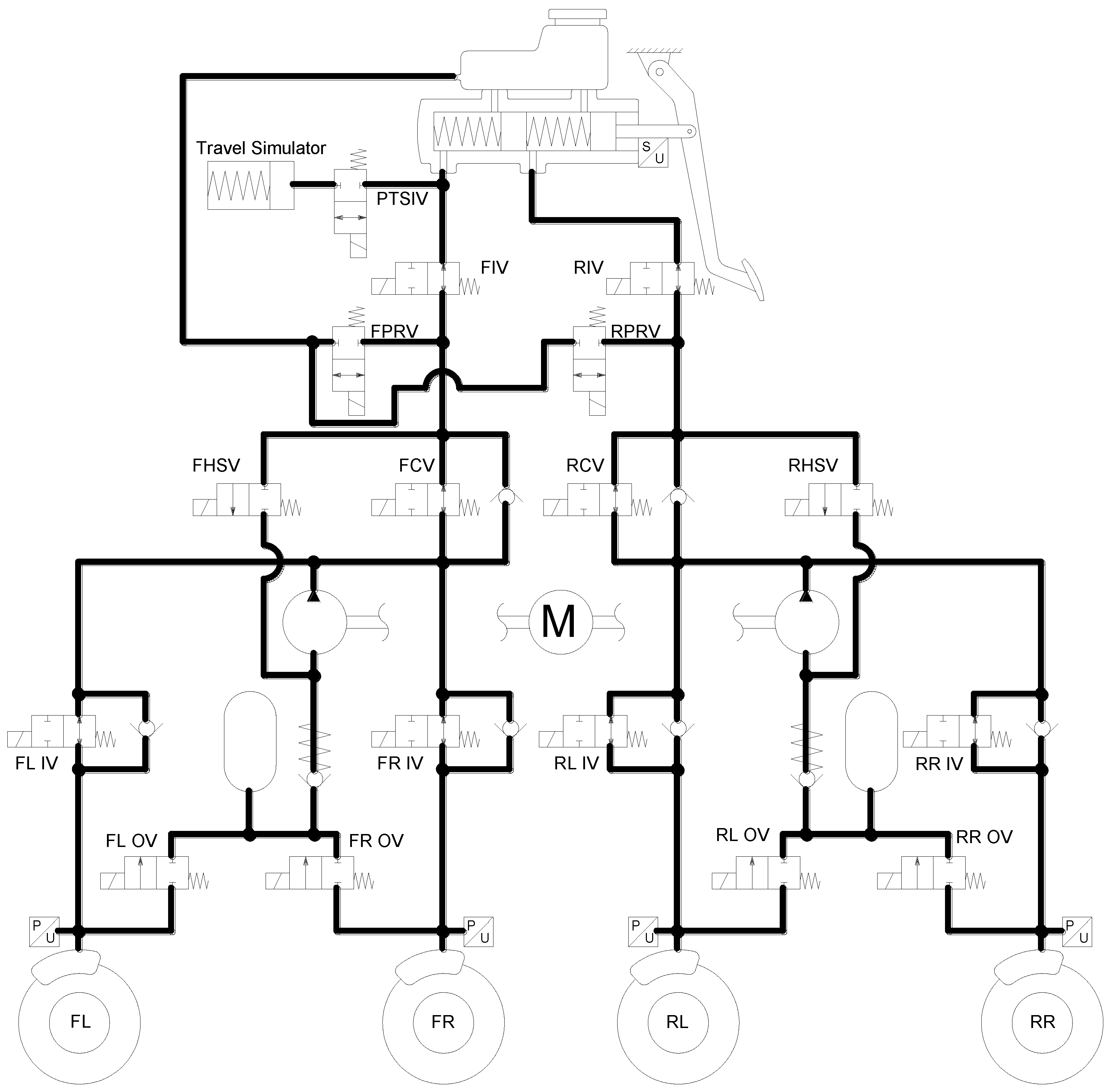
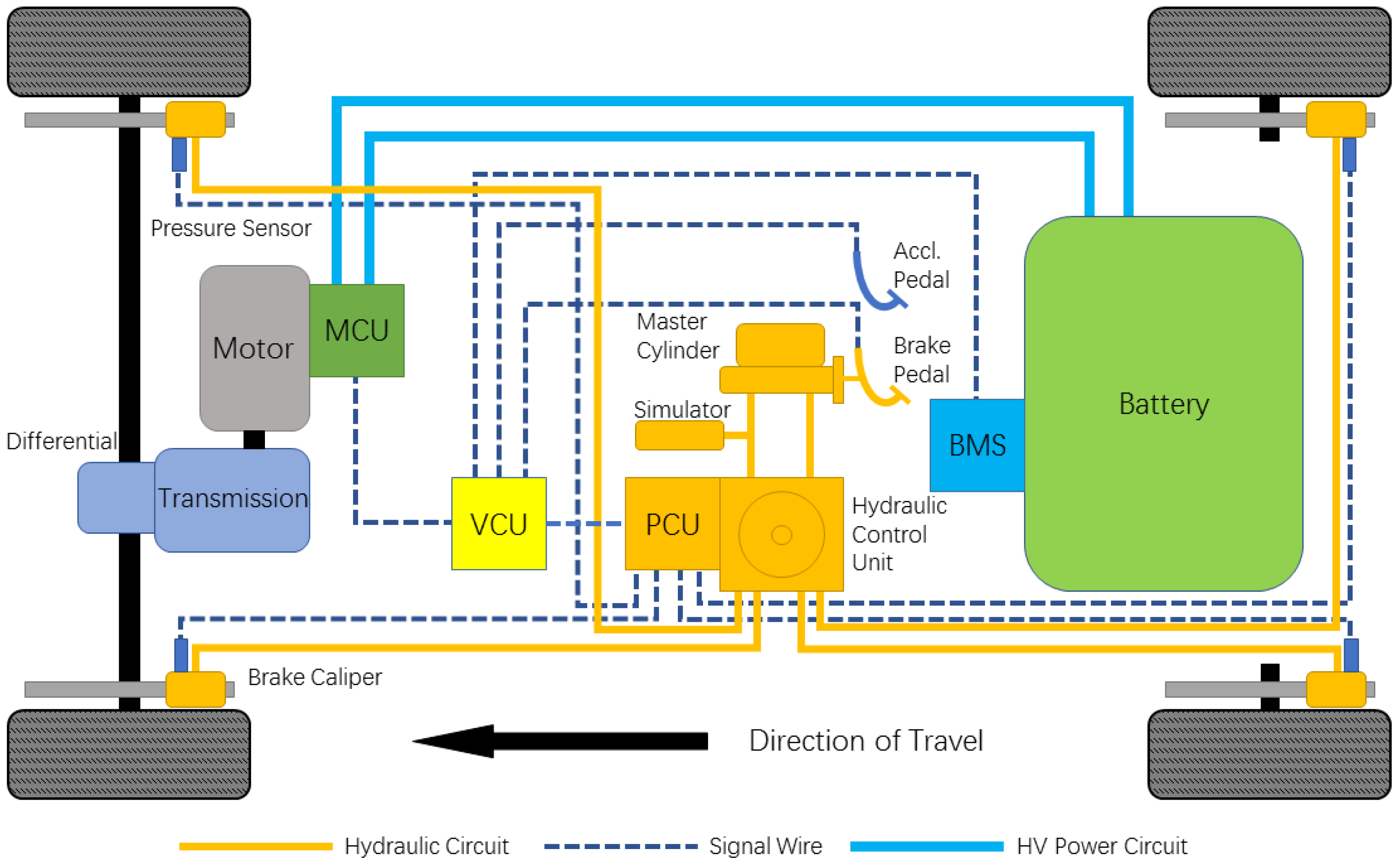
2.1. Design of the Mechanical Structure

In this study, the system was deployed on a front-wheel drive electric car and the layout is shown in Figure 1. The front axle was driven by a permanent magnet synchronous motor through a transmission with constant gear ratio and a differential. The motor was controlled by a motor control unit (MCU), which had driving logic and power electronics. A high-voltage lithium battery pack with battery management system (BMS) was used to provide energy for traction to propel the car and store the electric energy recovered. Each wheel was equipped with a disc brake with a hydraulic pressure sensor and the pressure in each brake cylinder was controlled by a hydraulic control unit, which was only had an actuator with some solenoid valves and electric pumps inside. An additional PCU (pressure control unit) was implemented to control the operation of the valves and pumps. All three control units (MCU, BMS, PCU) were connected to a vehicle control unit (VCU), which can recognize the driver’s intent by acquiring and analyzing the signals from the accelerator and brake pedals and control all the components by sending requests to other control units.

A detailed layout of the hydraulic braking system is shown in Figure 2. This consisted of a master cylinder assembly, a pedal travel simulation mechanism, a hydraulic control unit, and four brake calipers. The brake pedal was directly connected to the master cylinder instead of through a vacuum booster. A travel simulator was connected to the master cylinder through a normally closed solenoid valve called a pedal travel simulator isolation valve (PTSIV). This valve is designated as a safety device that can prevent the brake fluid from filling the travel simulator when the system is not powered. The travel simulator has a piston and two serially connected springs, which can be used to simulate the pressure-volume characteristic of the wheel cylinders by matching the stiffness and preload of the springs. For the remaining parts of the hydraulic brake system, the front and rear axles were identical in structure, so only the front axle is discussed. Through a front isolation valve (FIV), which will decouple the braking actuator from the braking control mechanism, the outlet port of the master cylinder is connected to an enhanced hydraulic control unit. In addition, a return line to the reservoir is also connected to the output port of the master cylinder, and this loop is controlled by the front pressure regulation valve (FPRV). The hydraulic control unit, marked by the dash line, is structurally similar to the hydraulic control unit in a conventional electronic stability control system. However, they are not identical as the hydraulic control unit in the proposed system has enhanced electric pumps that can meet the demand of a higher flow rate and longer working life. Therefore, a braking system such as that described above can control the braking force on each wheel independently, making it possible to implement torque vectoring control on the vehicle [15].

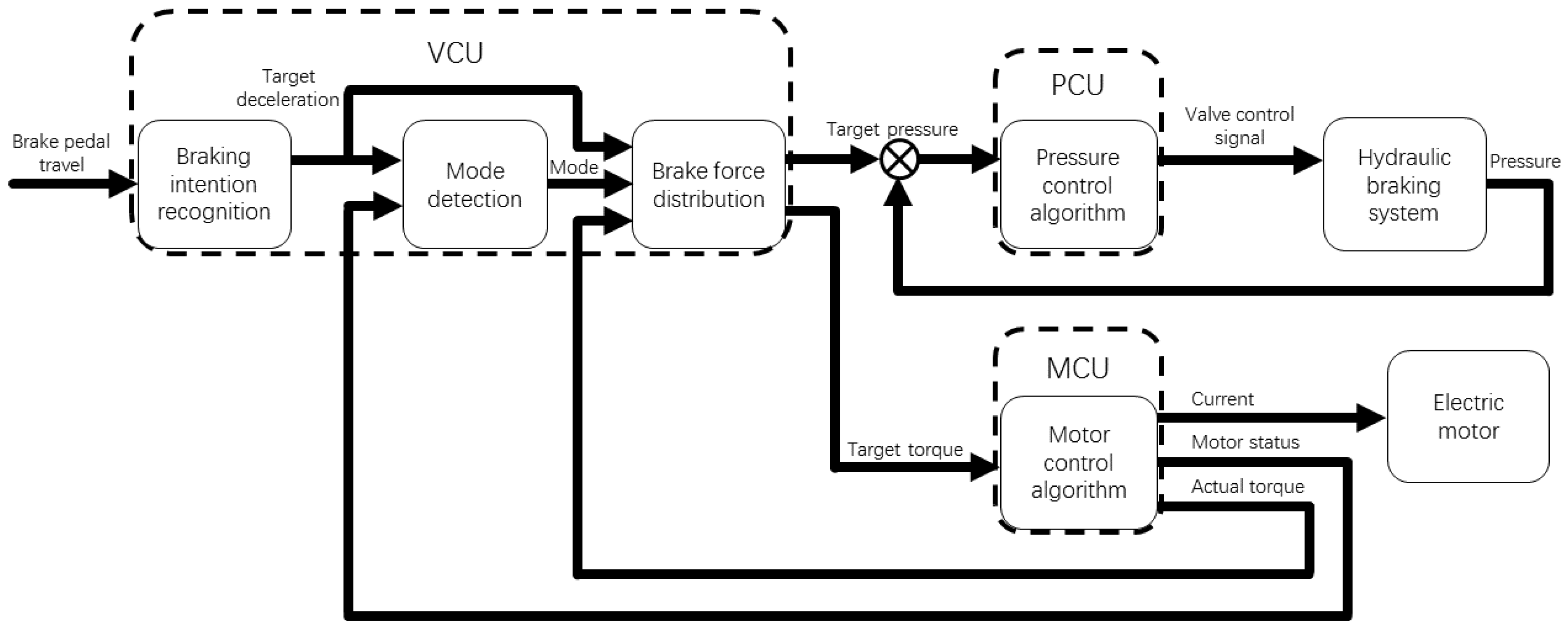
2.2. Design of the Cooperative Braking Controller

The block diagram of the controller for the cooperative braking system is shown in Figure 3. In this paper, the controller was embedded as a functional module in the VCU. The controller acquires the brake pedal travel as the input and recognizes the driver’s braking intention, which is then sent to the other two blocks. The mode detection block acquires the status of the motor as well as the target deceleration to find which mode the system should work in. Finally, the working mode and the demanded deceleration will be sent to the brake force distribution block to calculate the friction brake force on each axle produced by the motor. The friction brake force is converted to hydraulic pressure and is then sent to the PCU for pressure modulation. Meanwhile, the controller sends a motor torque request to the MCU to try to produce the calculated motor brake torque. Due to some limitations, however, the MCU may not produce enough braking force to meet the request, so it will send back the actual brake torque produced to the controller as feedback, which is then used to correct the brake force distribution.

2.2.1. Operation Modes of the Cooperative Braking System

The cooperative braking system has three operation modes: electric braking mode, cooperative braking mode, and hydraulic braking mode.

When the system is operating in the electric braking mode, the PTSIV will be at an open position to enable the pedal travel simulator while the front isolation valve (FIV) and rear isolation valve (RIV) will be in a closed position. All the brake fluid from the master cylinder flows into the pedal travel simulator. All other components of the hydraulic braking system will be kept in an idle state. The electric motor in the traction system will produce braking torque and recover electric energy into the battery.

For the cooperative braking mode, the electric motor and hydraulic braking system work together to apply braking force on the wheels. Like the electric braking mode, the electric motor performs regenerative braking and the pedal travel simulator is enabled. The difference is that the VCU will calculate the brake force distribution among the motor, front axle, and rear axle, and then send the pressure requests to the PCU to meet the driver’s demand for deceleration, simultaneously allowing the driver to obtain a similar brake feel to that on a conventional brake system. Meanwhile, the PCU will adjust the pressure in each brake cylinder by controlling the electric pumps and solenoid valves in the hydraulic control unit.

If the electric motor cannot recover energy, the system will work in only in the hydraulic braking mode. In this mode, the electric motor rotates with the wheels and outputs no braking torque and the hydraulic brake torque is distributed to the front and rear axles at a fixed ratio.

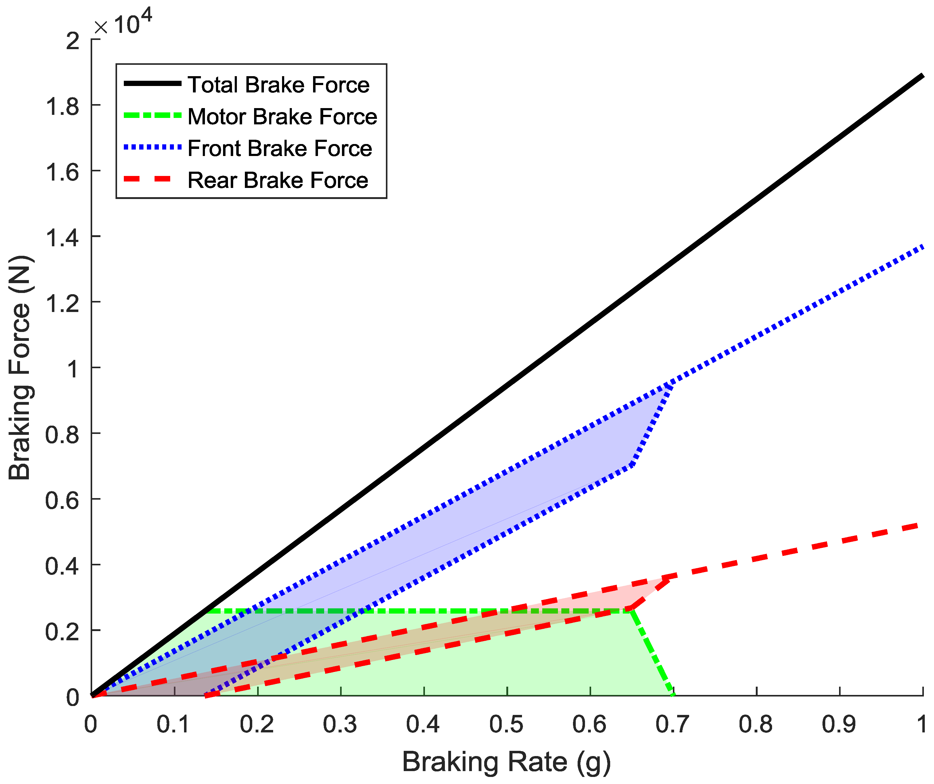
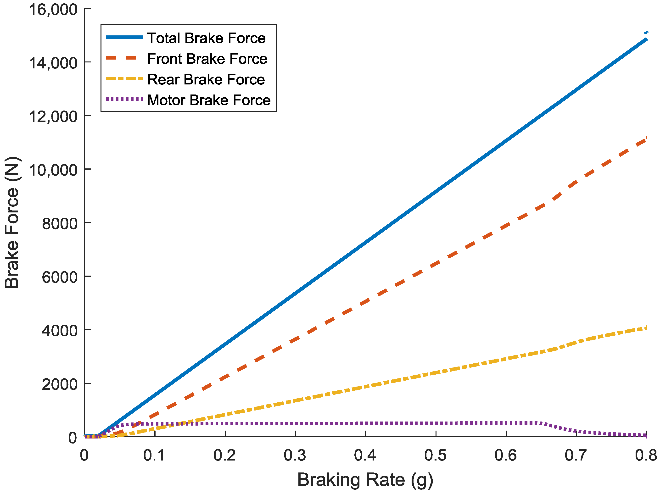
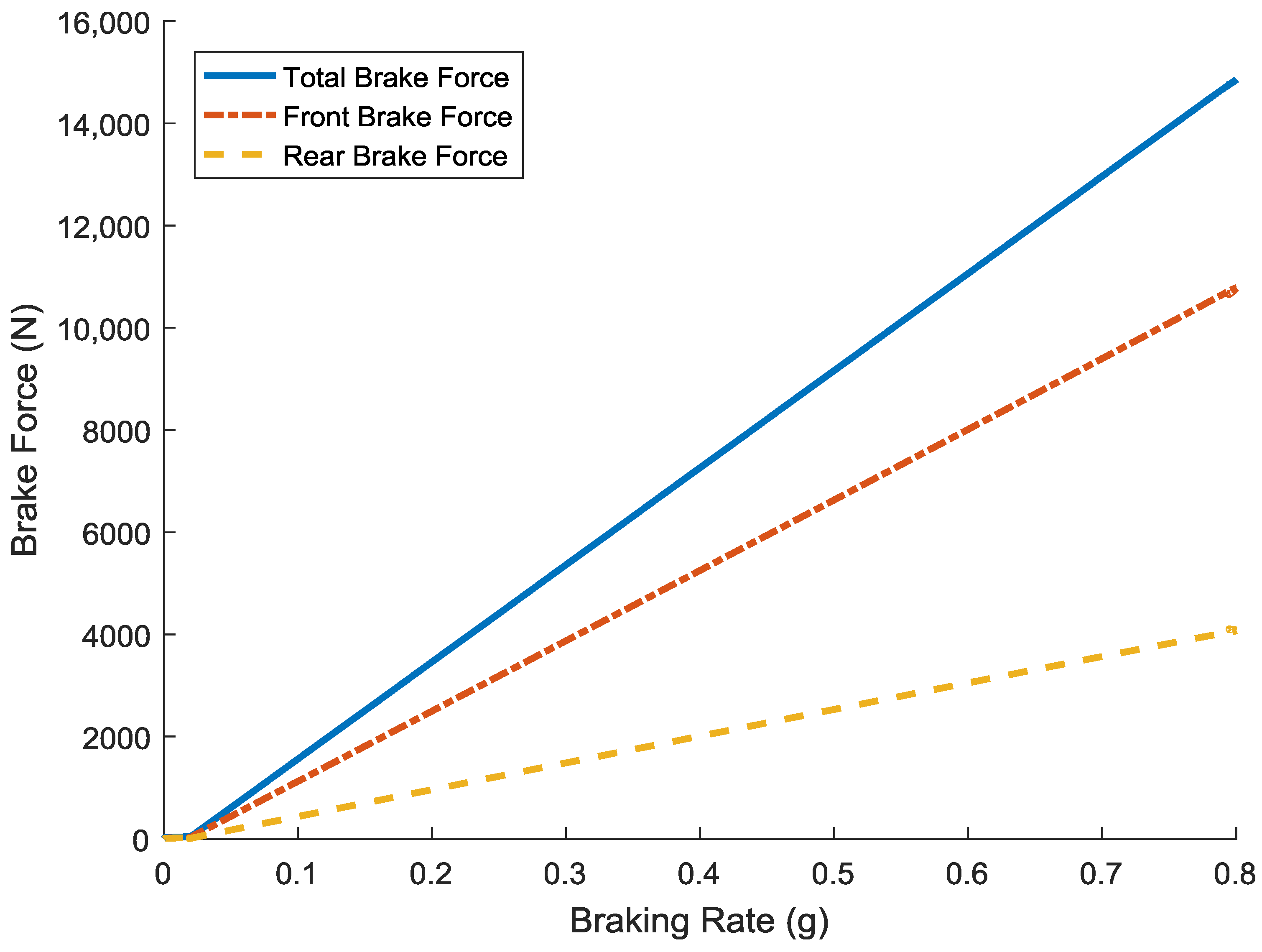
2.2.2. Brake Force Distribution Strategy in Cooperative Braking Mode

The braking force is distributed among the electric motor, the front brakes, and rear brakes to ensure that the total braking force meets the driver’s demand for deceleration. In previous studies, the most widely used braking force distribution strategy was the “the parallel strategy”, where the braking force is distributed at a fixed ratio between the motor, the front axle, and the rear axle. The advantage of this strategy is that it can be easily implemented in a conventional hydraulic braking system; however, it cannot maintain the deceleration of the vehicle when the brake pedal is held at a fixed position, nor will it maximize energy recovery [16]. In this paper, an improved braking force distribution strategy was proposed: the motor braking force was preferentially used, and the hydraulic braking force was adjusted in real time during the braking process so that the braking rate always followed the driver’s intention. The changes of braking forces with the braking rate is shown in Figure 4.

In this strategy, the distribution of the braking force is a range rather than a curve as the motor braking force will change within a certain range, and the front axle braking force and rear axle braking force will also vary within a range. The electric motor will be used as the only source of brake force when the braking rate is below 0.1368 G ($1.3406{\mathrm{ms}}^{-2}$), at which point the electric motor produces the maximum braking torque. When the braking rate extends beyond 0.1368 G, the controller will blend the motor braking force together with the hydraulic braking force to meet the driver’s braking demand. The electric motor will gradually withdraw from the braking process when the braking rate increases from 0.65 G to 0.7 G and will completely detach when it exceeds 0.7 G.

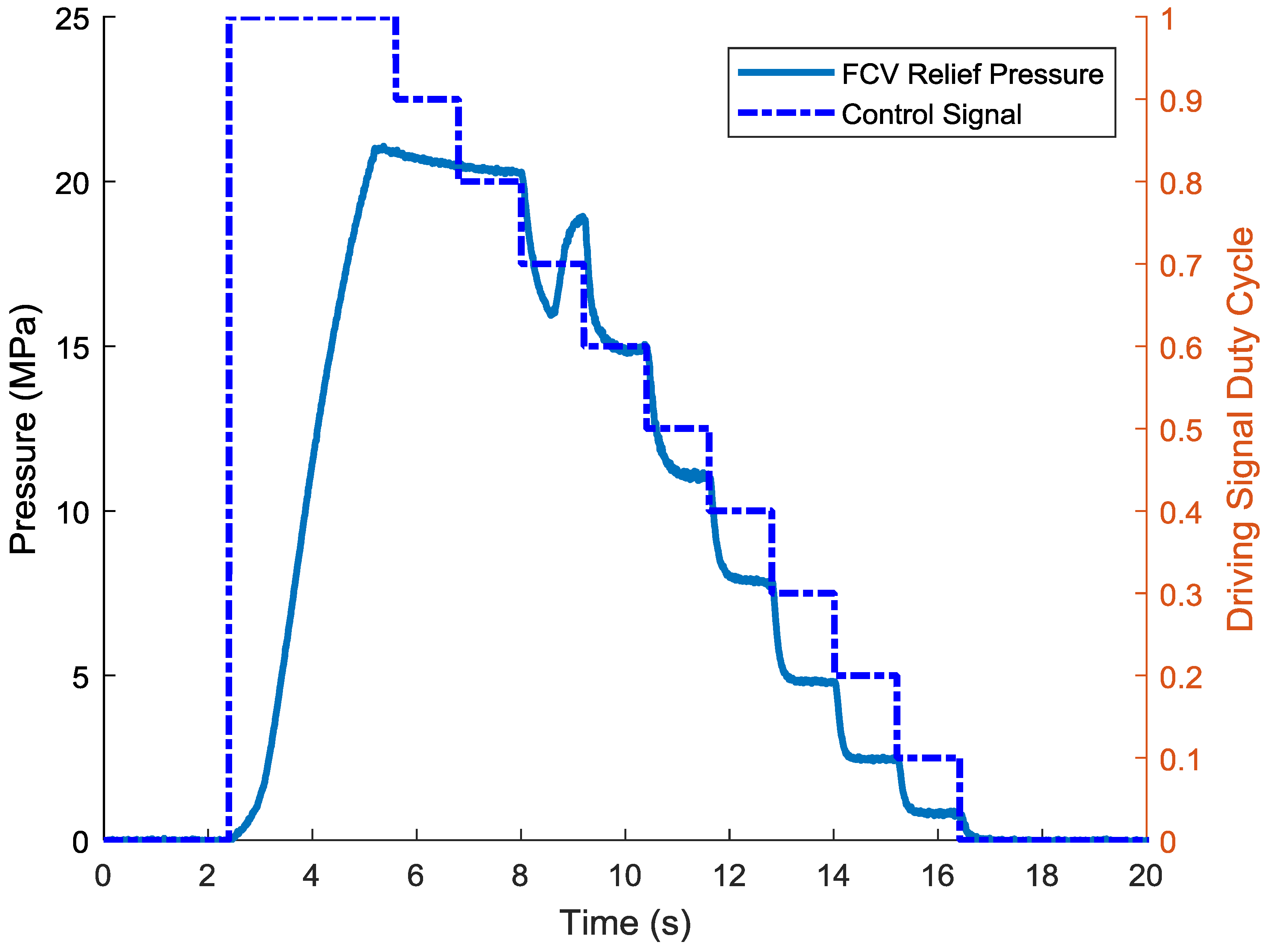
2.2.3. Pressure Control Method of the Hydraulic Braking System

Much research has been conducted on adjusting the brake wheel cylinder pressure through the solenoid valves and pumps and many control methods have been proposed. A widely-used control method is the PID (Proportional-Integral-Derivative)-bang-bang controller, which is quite simple to implement. However, this method cannot achieve a smooth braking process. This is acceptable in brake control systems that only work in emergency situations, but this method is not quite suitable for the system proposed in this paper, especially for the pressure increasing stage.

Some researchers have proposed a control method that uses the linear characteristics of inlet solenoid valves and have applied it in a traction control system [11,17]. In this method, the pressure increase rate can be controlled by adjusting the opening of the inlet solenoid valves, thus the pressure in the wheel cylinder can be controlled smoothly. Obviously, this method can achieve better control quality and can give the driver a smoother braking feel. However, according to the data in Kang’s study, a fact that can be inferred is that the relationship between opening the valves and pressure increase rate will change when the wheel cylinder pressure changes. Accordingly, it can be inferred that this method requires quite a large number of calibrations.

After studying the characteristics of the solenoid valves in the hydraulic control unit (HCU) by using the method and model proposed in Zhao’s paper [18], both the simulation and experiment proved that the front control valve (FCV) and rear control valve (RCV) had proportional relief characteristics, as illustrated in Figure 5. This means that a controllable constant pressure source can be realized by energizing the front/rear high-pressure switching valve (FHSV/RHSV) and adjusting the driving current of the FCV/RCV. The equivalent structure of the hydraulic braking circuit is shown in Figure 6. In this circuit, the FCV/RCV will work like proportional relief valves, thus the pressure at the output port of the pump can be controlled by adjusting the set pressure of the FCV/RCV. Hence, the authors proposed the use of a method that combined the control of the FCV/RCV and FIV/RIV to control the pressure in the wheel cylinders. This method will be quite simple to implement since it only needs a few calibrations, furthermore, it is foreseeable that the pressure regulation process will be smoother by using this method and will be suitable for a control process frequently triggered during daily driving.

3. Simulation Platform and System Components Modeling

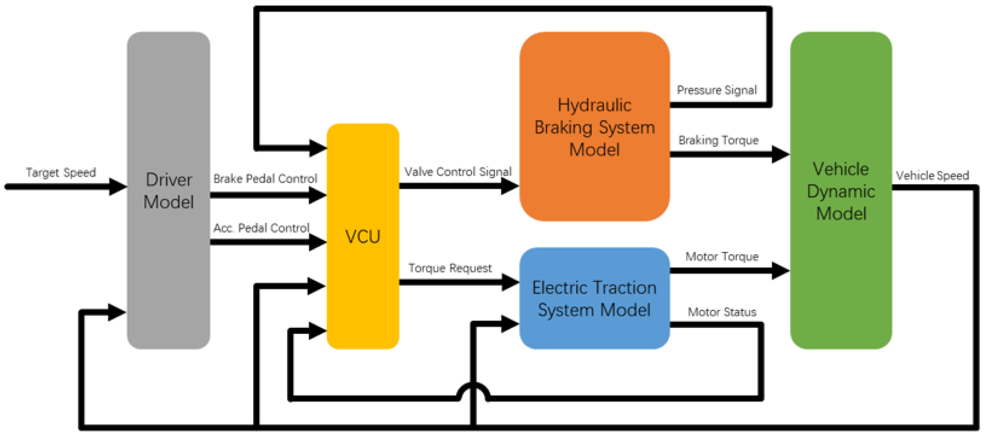
3.1. Structure of the Simulation Platform

To conduct simulations and analyze the characteristics of the system, a simulation platform was built in Simulink as shown in Figure 7. This consisted of five sub systems: the hydraulic braking system, the traction system, the vehicle, the controller, and a simple proportional–integral (PI) driver model that accepts the speed input and outputs the brake pedal and acceleration pedal travel signal.

3.2. Vehicle Dynamic Modeling

Since only longitudinal motion and axle load transfer were considered, a simple longitudinal vehicle model was established. Aerodynamic drag force is also one of the main driving resistances, especially in high-speed driving conditions. To evaluate the effect of energy recovery more accurately, the aerodynamic drag was not ignored. Force in the longitudinal direction of the car can be described as:

$$m\dot{v}=F_1+F_2-F_a$$

(1)

where $F_1$ and $F_2$ are the longitudinal tire forces of the front and rear wheels, respectively; $F_a$ is the aerodynamic drag force; $m$ is the mass of the car; and $v$ is the speed of sprung mass. Aerodynamic drag is one type of force that needs to be overcome by the vehicle while moving and significantly affects the energy efficiency of the vehicle [19]. Aerodynamic drag can be calculated by the following equation:

$$F_a=\frac{1}{2}{C}_{d}A\rho v^2$$

(2)

where $C_d$ is the drag coefficient; $A$ is the reference area; and $\rho$ is the mass density of air.

3.2.1. Tire Modeling

Almost all the external forces—with the exception of aerodynamic—exerted on the car are from the contact surface between the tires and ground. Since tire modeling is so important in vehicle dynamic modeling, a lot of research has been conducted in this area and many modeling methods have been discovered. Among these tire models, the “magic formula” is the most widely used and has become the de facto industry standard. More tire manufacturers have begun to provide customers with magic formula parameters. In this study, the tires were modeled using the “magic formula” and can be presented as:

$$F_i=F_{xi}-f{F}_{zi}$$

(3)

$$F_{xi}=D\sin \left(C{\mathit{tan}}^{-1}\left\{B{s}_i-E\left[B{s}_i-{\mathit{tan}}^{-1}\left(B{s}_i\right)\right]\right\}\right)F_{zi}$$

(4)

where $F_{zi}$ and $s_i$ are the normal load of the tire and slip rate, respectively. $F_{xi}$ is the longitudinal force exerted on the tire. $B$, $C$, $D$, and $E$, which are constants, are the parameters of the magic formula, and the meanings are described in Pacejka [20]. The coefficient of rolling resistance, which is presented as $f$ in Equation (4), is regarded as speed independent, therefore it is a constant. From the tire model, the tire force is affected by the normal load. As the vehicle acceleration changes, the vertical load will be transferred between the two axles, and the load transfer can be expressed as:

$$F_{z1}=\frac{mg}{L}\left(L_2-\frac{\dot{v}{h}_g}{g}\right)$$

(5)

$$F_{z2}=\frac{mg}{L}\left(L_1+\frac{\dot{v}{h}_g}{g}\right)$$

(6)

where $g$ is the gravity constant; $L$ is the wheel base, and it is assumed that the front axle and rear axle have the same wheel base. $L_i$ is the distance from the front or rear axle to the gravity center and $h_g$ is the height of the gravity center.

3.2.2. Wheel Modeling

Since the car described herein is a front-wheel drive car, the wheels were divided into drive wheels and driven wheels. In addition to the force between the tire and the ground, the torque output from the axle as well as the braking torque generated by the brake calipers and motor were also applied to the drive wheel. Therefore, the force balance on the drive wheels can be described as:

$$\left(J_{w1}+\frac{J_{m1}}{2i^2}\right)\dot{{\omega }_1}=\frac{1}{2}\left(T_{m1}-R{F}_1-T_{h1}\right)$$

(7)

$$T_{m1}=i{T}_m$$

(8)

where $J_{w1}$ is the moment of inertia of one front wheel; and $J_{m1}$ is the moment of inertia of the electric motor’s rotor. The front wheels were driven through a transmission and the gear ratio was $i$. $T_m$ is the motor torque; $R$ is the rolling radius of the wheel; ${\omega }_1$ is the angular speed of the wheel; $T_{h1}$ is the hydraulic braking torque on the front axle; and $T_{m1}$ is the driving torque output by the motor through the transmission. The rolling radius was regarded as a constant and the moment of inertia of transmission ignored.

For driven wheels, there is no driving torque exerted on them, so the force balance on them can be presented as:

$$J_{w2}\dot{{\omega }_2}=\frac{1}{2}\left(-R{F}_2-T_{h2}\right)$$

(9)

where $J_{w2}$ is the moment of inertia of the rear wheel; and $T_{h2}$ is the hydraulic braking torque of the rear wheel.

Braking torque exerted on each wheel can be expressed as:

$$T_{Bi}=P_i{A}_i{C}_{BF}{R}_{Ei}$$

(10)

where $T_{Bi}$ is the brake torque applied on a wheel; $P_i$ is the pressure of the brake fluid in a wheel cylinder and $A_i$ is the sectional area; $C_{BF}$ is the brake factor of a disc brake, usually double the friction coefficient; and $R_E$ is the effective radius of the brake disc.

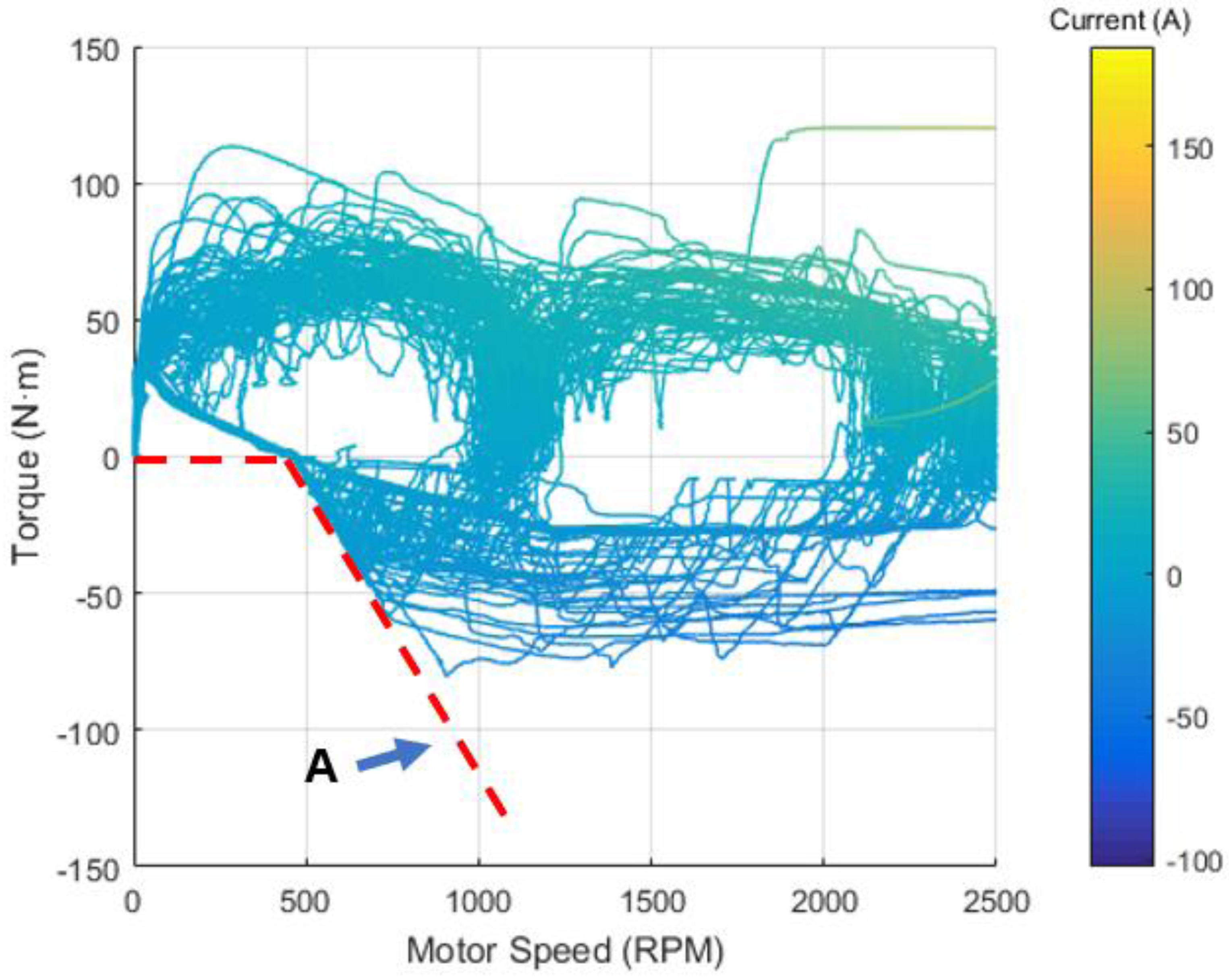
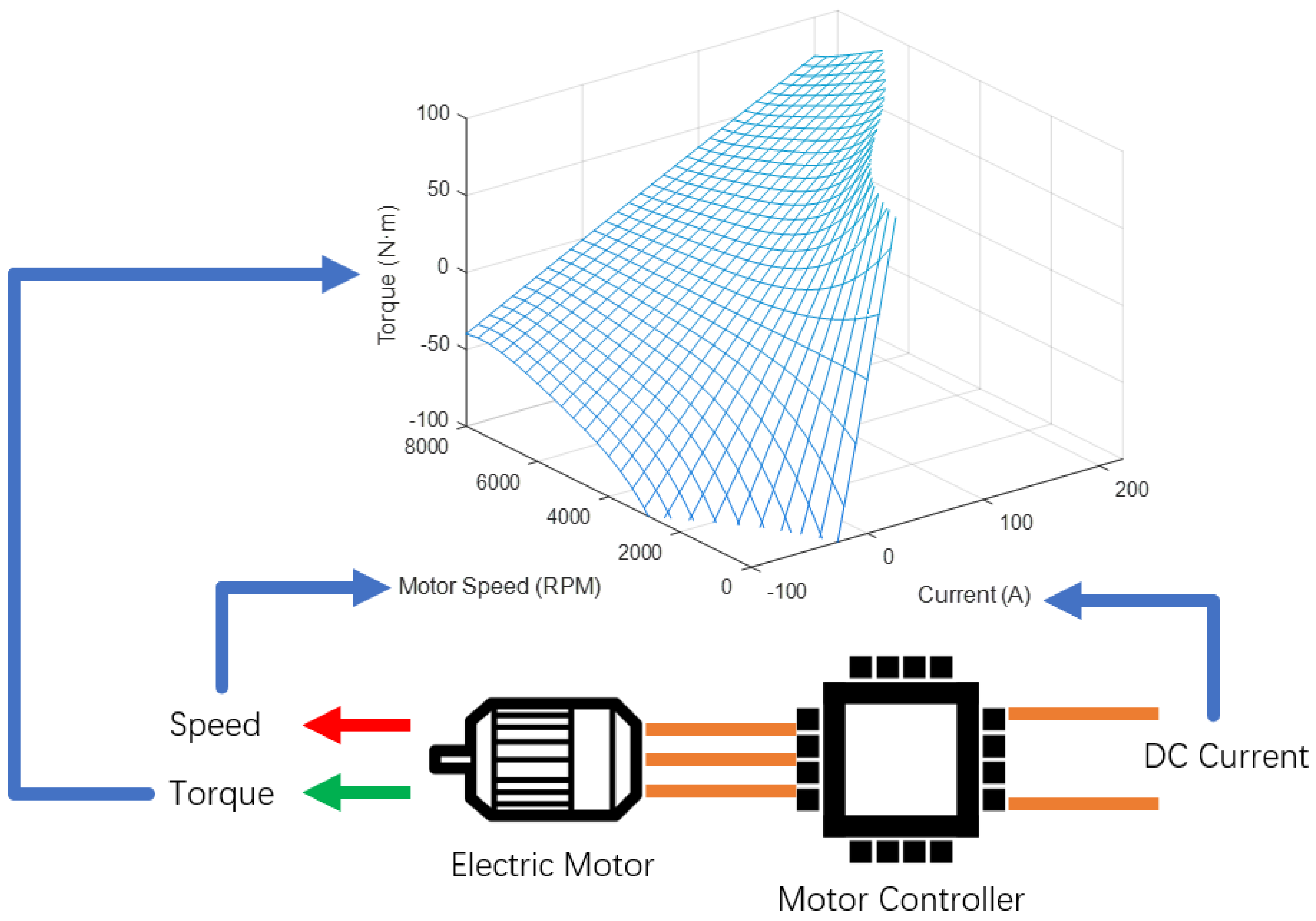
3.3. Traction System Modeling

The traction system mainly consisted of three parts: the electric motor, the motor controller, and the battery. Higher model complexity can achieve higher simulation accuracy, but it usually requires more parameters to be calibrated and is not easy to achieve. On the other hand, excessive simplification of the simulation model may lead to misleading results. To simplify the model and make the model sufficiently accurate, a steady-state black box model where the motor controller and motor are regarded as a whole component, was established based on the experimental data. Since only limited data points were acquired, to obtain a better simulation model, the data points were fitted as the following polynomial function and is shown in Figure 8:

$$T_{m\_current}(I_m,{\omega }_m)={\displaystyle \sum }_{i=0}^m{\displaystyle \sum }_{j=0}^n{P}_{ij}{I_m}^i{{\omega }_m}^j$$

(11)

where $I_m$ is the current on the DC bus; ${\omega }_m$ is the motor speed; and $P_{ij}$ is the constant coefficient.

The motor controller receives the torque command from the VCU during operation, after that it drives the motor to produce the requested torque. The regenerative braking torque is generated by the back EMF (electromotive force), so it will be limited at low speed [21]. An experiment was undertaken to find the maximum regenerative braking torque when the motor is running at low speed, the result is shown in Figure 9. The dashed line marked as “A” shows the boundary of the regenerative braking torque.

Thus, when the motor is running at low speed, the maximum regenerative braking torque can be calculated by using the following equation:

$$T_{m\_speed}\left({\omega }_m\right)=a{\omega }_m+b$$

(12)

where $a$ and $b$ are the constant coefficients that can be obtained through experiments. When the electric motor is running at higher speed, the maximum torque it can output is limited by the maximum charging or discharging current of the battery, which can be calculated by using Equation (11).

The motor controller accepts torque requests from the CAN (Controller Area Network) bus and drives the electric motor to reach the requested torque when it does not exceed the torque limitation. If the requested torque goes beyond the limitation at a certain working point, then the maximum torque will be output to the transmission. In summary, the responded motor torque at a certain motor speed can be defined as:

$$T_m=\{\begin{array}{c}min\left[T_{m\_speed}\left({\omega }_m\right),T_{m\_current}\left(I_{b\_disc\_max},{\omega }_m\right),T_{req}\right]\left(T_{req}\ge 0\right)\\ max\left[T_{m\_speed}\left({\omega }_m\right),T_{m\_current}\left(I_{b\_char\_max},{\omega }_m\right),T_{req}\right]\left(T_{req}<0\right)\end{array}$$

(13)

where $I_{b\_disc\_max}$ is the maximum discharging current; $I_{b\_disc\_max}$ is the maximum charging current; and $T_{req}$ is the requested motor torque sent from the VCU.

3.4. Battery Modeling

A simplified battery model was used in this research, and can be expressed as the following equation:

$$SOC=SO{C}_0-\frac{{{\displaystyle \int }}_0^{\tau }{\eta }_b{I}_m\left(\tau \right)d\tau }{Q_c}$$

(14)

where $SOC$ and $SO{C}_0$ are the actual and initial state of charge of battery pack; $Q_c$ is the total energy capacity of the battery pack; and ${\eta }_b$ is the charging or discharging efficiency of the battery.

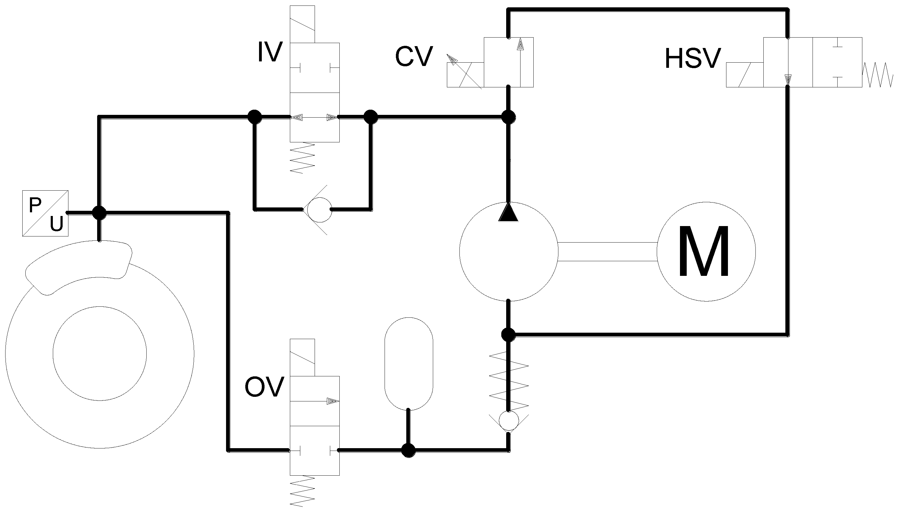
3.5. Hydraulic Braking System Modeling

As shown in Figure 2, the hydraulic braking system consisted of the master cylinder assembly, travel simulator, hydraulic control unit, and brakes. These components were modeled to conduct simulations to evaluate the performance and characteristics of the system.

3.5.1. Hydraulic Control Unit Modeling

The hydraulic control unit is a device characterized by twelve solenoid valves, two accumulators, and two pumps. This device can control the hydraulic pressure in each brake caliper independently through the controlling pumps and solenoid valves. Since the layout of the hydraulic braking system discussed in this paper was “axle by axle”, only the front braking circuit modeling is discussed, and the rear circuit can be modeled in the same way. As described above, the FCV can be treated as a solenoid proportional relief valve, so the relief pressure of FCV is a function of the input current on the solenoid expressed as:

$$P_{FCV}=a_0{I_{FCV}}^3+a_1{I_{FCV}}^2+a_2{I}_{FCV}+a_3$$

(15)

where $P_{FCV}$ is the relief pressure of the FCV, $I_{FCV}$ is the current in the solenoid of the FCV. $a_0$, $a_1$, $a_2$ and $a_3$ are constants that can be achieved through experimental tests.

When the relief pressure changes, the pressure at output port of the pump will take some time to stabilize, and this process can be expressed as:

$$P_s\left(s\right)=\frac{{\omega }_{np}}{s^2+2{\xi }_p{\omega }_{np}s+{\omega }_{np}}{P}_{FCV}\left(s\right)$$

(16)

where $P_s\left(s\right)$ is the pressure at the output port of the pump and $P_{FCV}$ is the relief pressure.

When the HCU is regulating the pressure in the front left wheel cylinder, the brake fluid flowing out of the hydraulic pump flows into it through the FLIV (front-left inlet valve) and flows out of it through the FLOV (front-left outlet valve), before finally going into the front low-pressure accumulator. Therefore, the flow rate of the brake fluid flows into the front left wheel cylinder can be calculated using the following equation:

$$Q_{FL}=D_{FLIV}{C}_{FLIV}\sqrt{P_s-P_{FL}}-D_{FLOV}{C}_{FOV}\sqrt{P_{FL}-P_{FA}})$$

(17)

where $Q_{FL}$ is the flow rate; $D_{FLIV}$ and $D_{FLOV}$ are the control signals of FLIV and FLOV; and $C_{FLIV}$ and $C_{FLOV}$ are the flow coefficients of FLIV and FLOV. $P_{FL}$ and $P_{FA}$ represent the pressure of the front left wheel cylinder and front low-pressure accumulator, respectively. Furthermore, in a certain period, the volume that flows into or out of the wheel cylinder can be expressed as:

$$V_{FL}={{\displaystyle \int }}_0^t{Q}_{FL}\left(\tau \right)d\tau$$

(18)

where $V_{FL}$ is the volume of brake fluid flow into or out of the front left wheel cylinder.

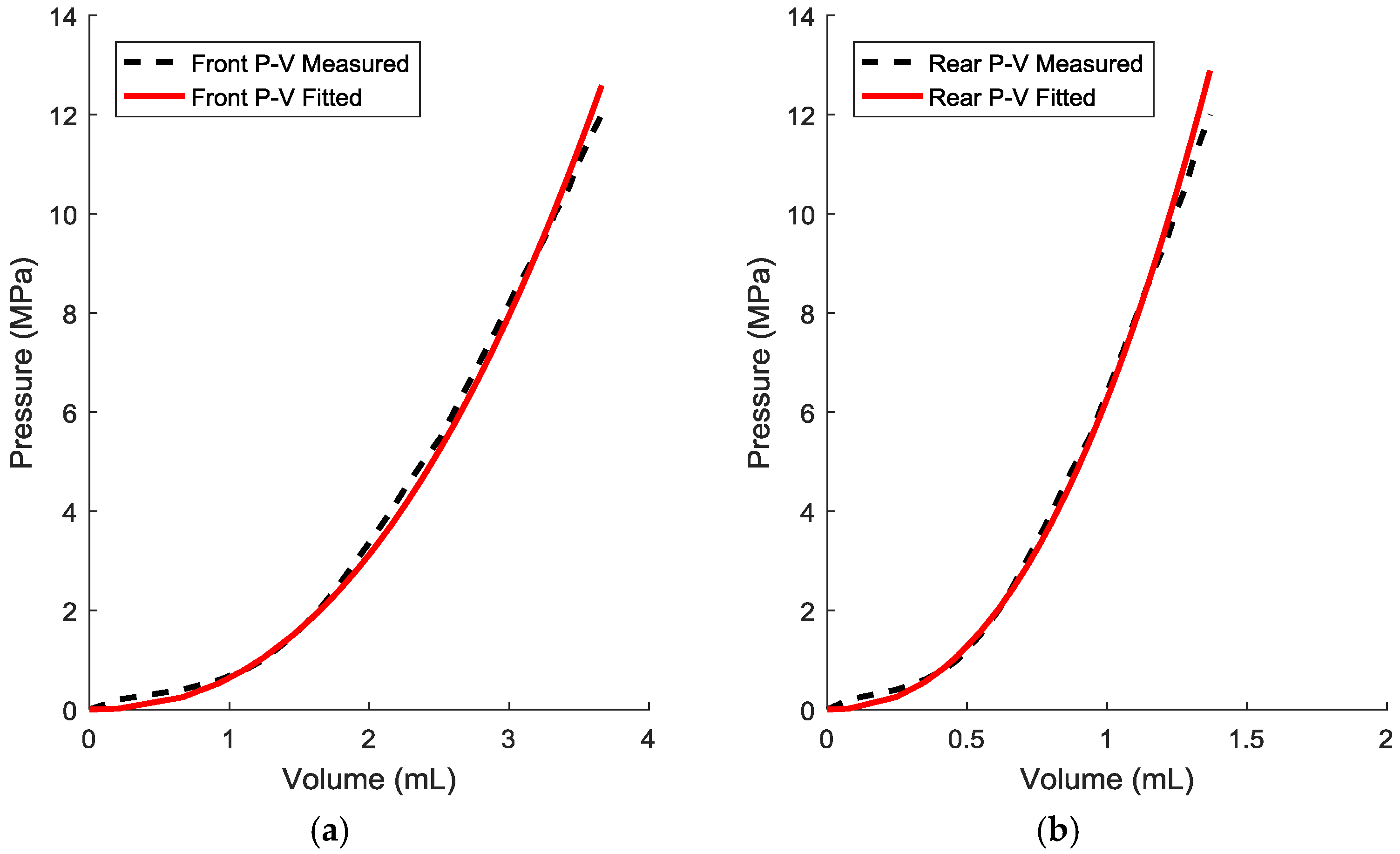
3.5.2. Brake Caliper Modeling

Modeling brake calipers based on mechanical structures is cumbersome since the deformation of the caliper bodies and brake pads are hard to measure and estimate. Therefore, the brake calipers were modeled based on pressure-volume characteristics, which can be measured easily through experiments. The P-V characteristics of the front and rear calipers are shown in Figure 10. The measured data can be fitted to a curve represented by Equation (19) [22]:

$$P_i={\gamma }_i{V_i}^{{\lambda }_i}$$

(19)

where $P_i$ is the pressure of the brake cylinders at the front or rear axle, and ${\gamma }_i$, ${\lambda }_i$ are coefficients of pressure-volume characteristics that can be fitted through the experimental data.

3.5.3. Master Cylinder and Pedal Assembly Modeling

A tandem master cylinder was modeled in this paper. The input push-rod of the master cylinder was connected directly to the pedal assembly instead of through a booster. The pressure in the master cylinder and the force applied on the brake pedal can be represented as:

$$F_P=\frac{1}{R_P}\left(P_{MC}{A}_{MC}+S_{MC}{k}_{MC}+L_{MC}\right)$$

(20)

where $P_{MC}$ is the pressure of brake fluid in the master cylinder; $A_{MC}$ and $S_{MC}$ are the sectional area and piston stroke of master cylinder, respectively; and $k_{MC}$ and $L_{MC}$ are the stiffness and preload of the spring in it. $F_P$ is the force applied on the brake pedal and $R_P$ is the leverage ratio of brake pedal.

3.5.4. Brake Pedal Travel Simulator Modeling

The brake pedal travel simulator is a component that can simulate the pressure-volume characteristics of the brake calipers. By deploying such a device in the hydraulic circuit, the brake pedal maintains a smooth pedal feel when the HCU is regulating pressure in each brake. The pedal travel simulator is a spring cylinder with two springs of different stiffness, and the two springs are connected in series. Each spring is preloaded respectively, and the preload of the second spring equals the force of the first spring at maximum compression. Therefore, when the first sprint is being compressed, the pressure-volume characteristics of the travel simulator can be calculated by using the following equation:

$$P_S=\frac{1}{A_S}\left(L_{s1}+K_{s1}\frac{V_S}{A_S}\right)$$

(21)

where $P_S$ is the pressure of the brake fluid in the brake pedal travel simulator; $A_S$ is the sectional area of it; $L_{s1}$ and $K_{s1}$ are the preload and stiffness of the first spring, respectively; and $V_S$ is the volume of brake fluid flow into the simulator.

When the first spring reaches maximum compression, the second spring will be compressed and the pressure-volume characteristics will be:

$$P_S=\frac{1}{A_S}\left(L_{s2}+K_{s2}\left(\frac{V_S}{A_S}-\frac{L_{s2}-L_{s1}}{K_{s1}}\right)\right)$$

(22)

where $L_{s2}$ and $K_{s2}$ are the preload and stiffness of the second spring, respectively.

4. Verification and Analysis of the System in Simulation Environment

Several experiments were carried out in a simulation environment to verify the feasibility and effectiveness of the system. The main parameters used in the simulations are shown in

Table 1. Main parameters used in simulations.

Parameter	Value
Total weight of the car	$1928\mathrm{kg}$
Wheelbase	$2675\mathrm{mm}$
Distance from front axle to centroid	$1263\mathrm{mm}$
Distance from rear axle to centroid	$1412\mathrm{mm}$
Centroid height	$530\mathrm{mm}$
Drag area	$0.6789{\mathrm{m}}^2$
Moment of inertia of a wheel	$1.12\mathrm{kg}·{\mathrm{m}}^2$
Rolling radius of a wheel	$0.308\mathrm{m}$
Transmission reduction ratio	$8.28$
Battery capacity	$43,200\mathrm{C}$
Initial SOC(state of charge)	$80\%$
Brake factor	$0.7$
Diameter of front wheel cylinder	$57.15\mathrm{mm}$
Diameter of rear wheel cylinder	$34.92\mathrm{mm}$
Diameter of master cylinder	$18\mathrm{mm}$
Effective radius of front brake rotor	$0.225\mathrm{m}$
Effective radius of rear brake rotor	$0.230\mathrm{m}$
Brake pedal leverage ratio	$3.5$
Diameter of pedal travel simulator	$15\mathrm{mm}$
Stiffness of pedal travel simulator spring (1st stage)	$9.03\mathrm{N}/\mathrm{mm}$
Stiffness of pedal travel simulator spring (2nd stage)	$42.16\mathrm{N}/\mathrm{mm}$

.

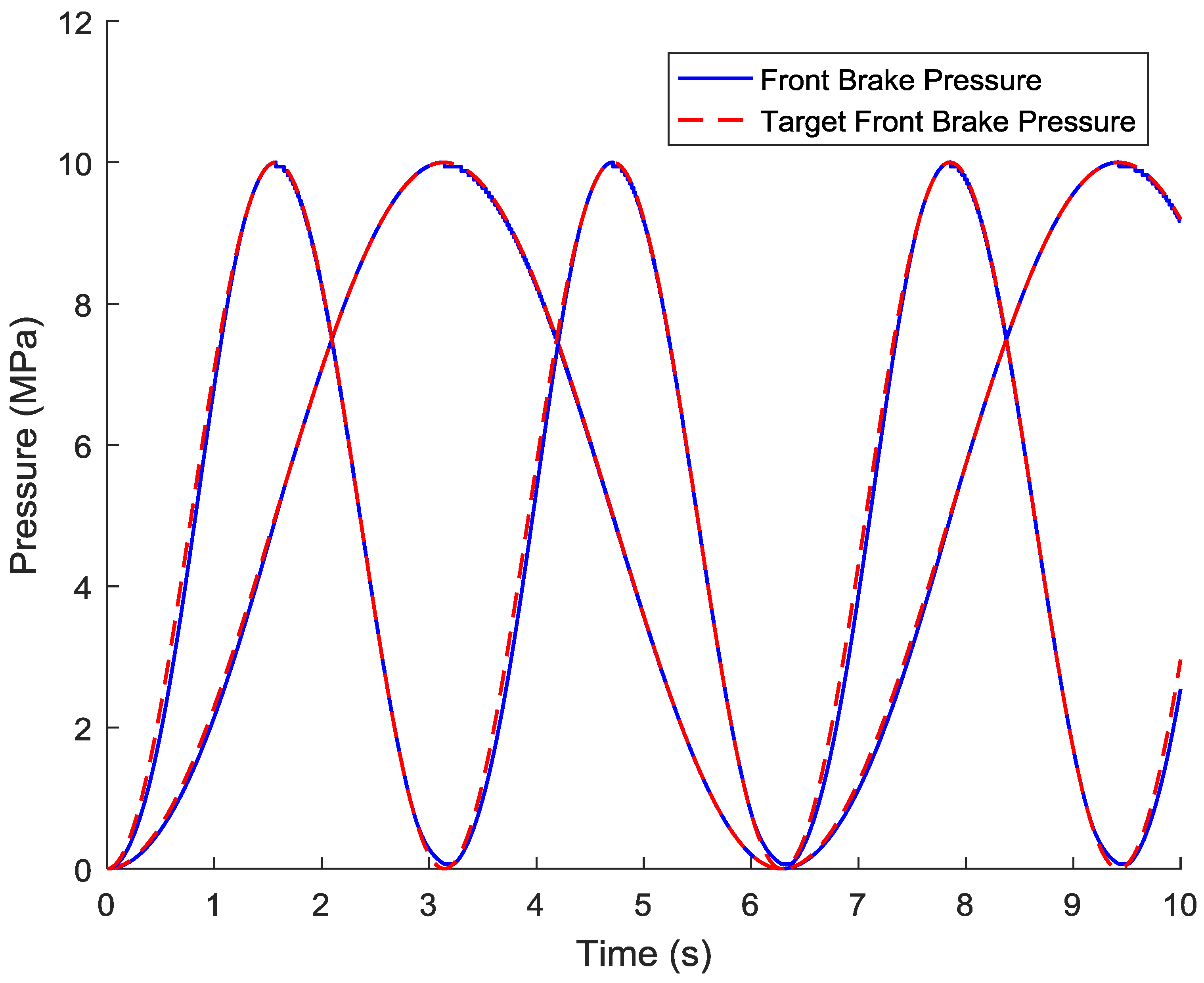
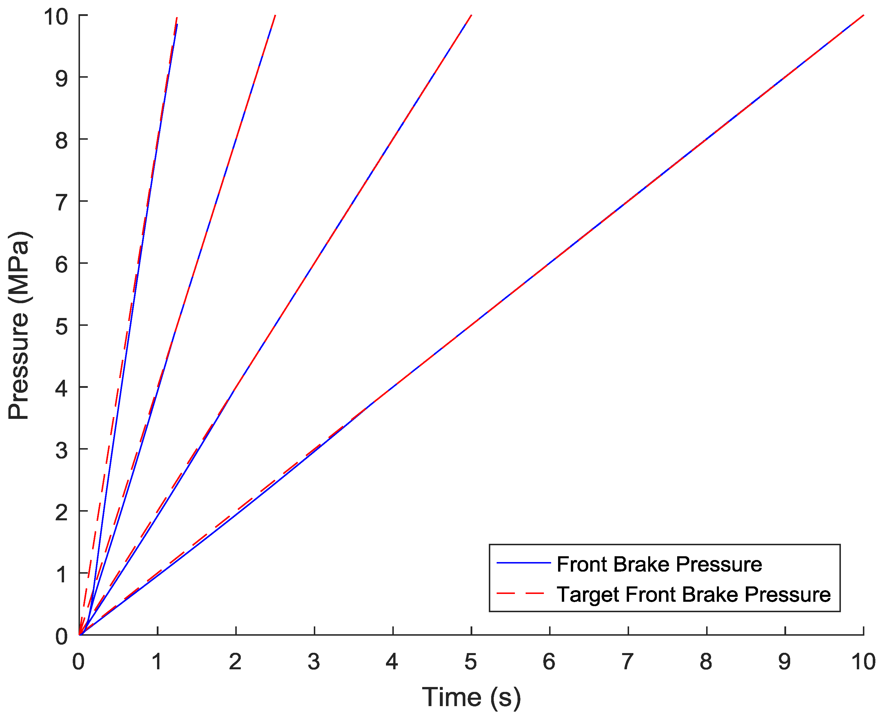
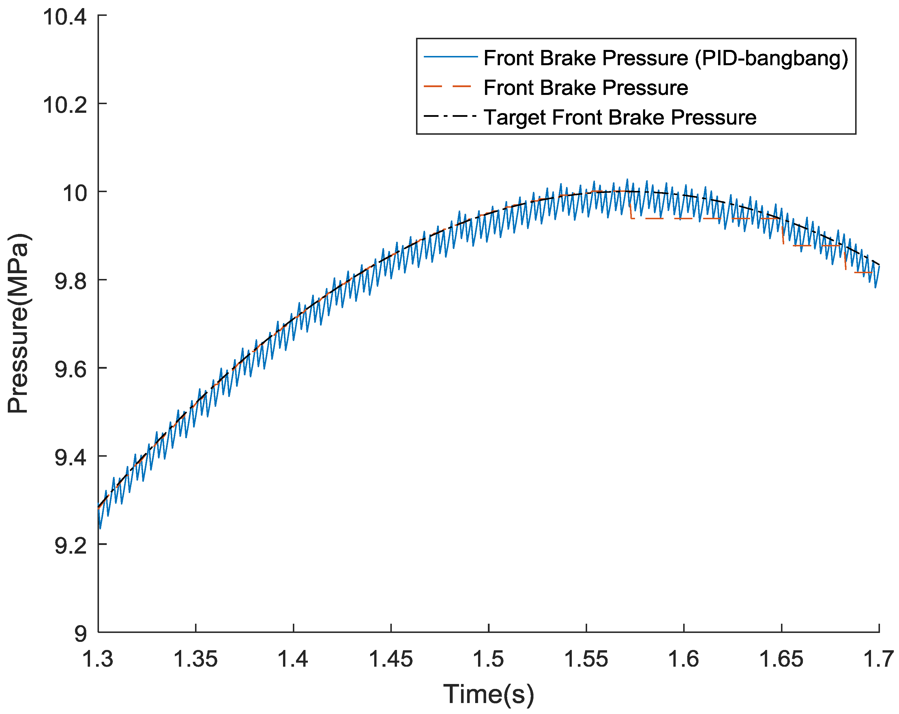
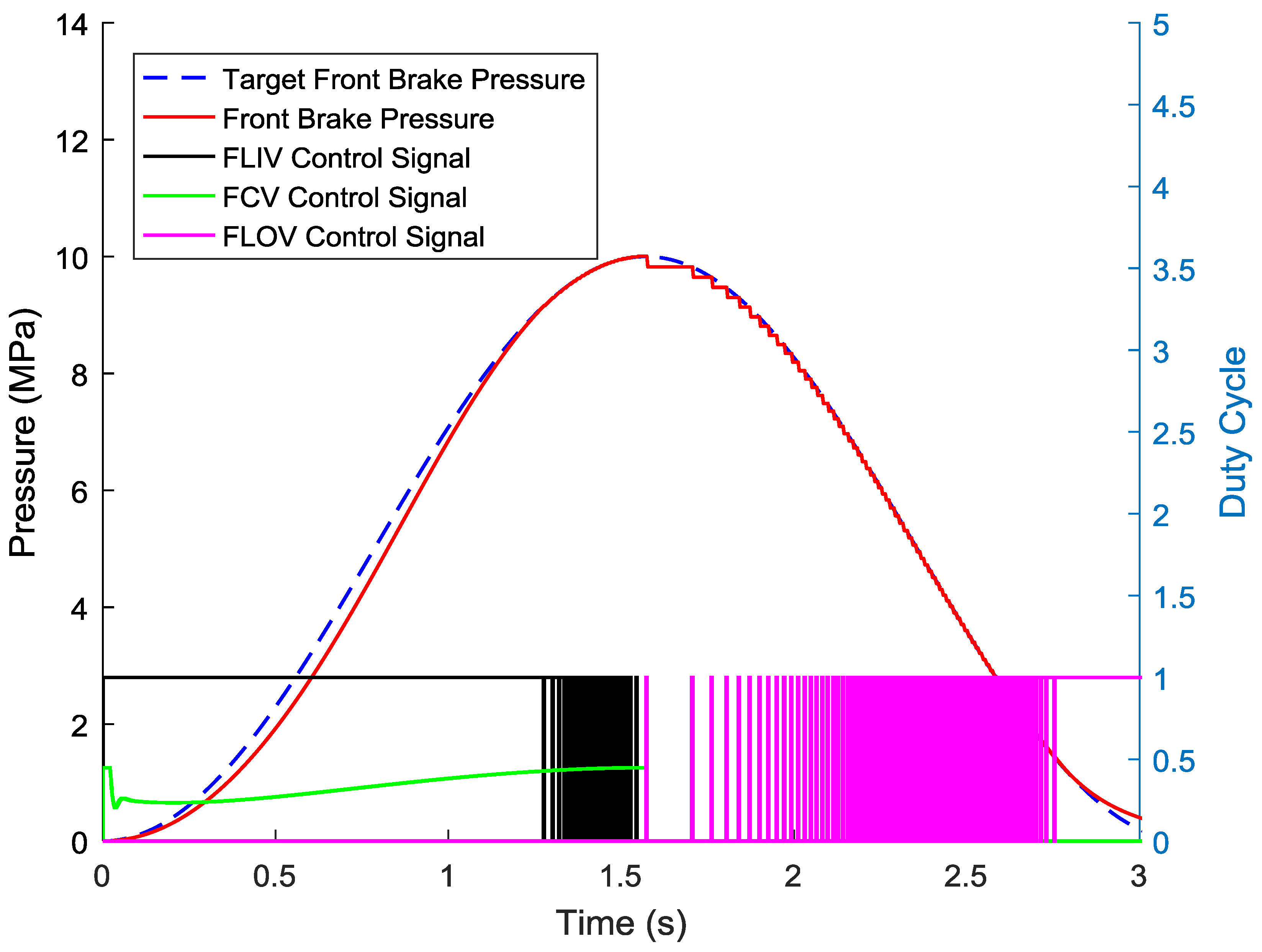
4.1. Simulation and Analysis of Wheel Cylinder Pressure Modulation Algorithm

To maintain a stable braking rate while the electric motor intervenes in the braking process, the hydraulic control unit will regulate the pressure in each wheel cylinder. The dynamic characteristics of the hydraulic control unit is a key factor of this pressure regulation process and can be obtained by observing the ramp response and sinusoidal response of the hydraulic braking system [8]. The simulation results are shown in Figure 11 and Figure 12. In Figure 11, two curves, excited at two different frequencies, show that the hydraulic control unit could regulate the pressure in the wheel cylinders with relatively high precision when working in the pressure increasing stage. However, there will be a delay during the regulation process, which is mainly caused by the brake caliper gap and the flow rate limitation of the valves. Unlike the delay shown in the pressure increasing stage, when working at the pressure decreasing stage and the pressure is higher than 7 MPa, there will be an overshot in the pressure decrease stage, which is caused by the excessive pressure difference and fixed control cycles of the outlet valves.

For the ramp response test, the conclusion was almost the same as that in the sinusoidal response test where it was obvious that the delay of the low-pressure portion increased as the target pressure rate increased. Figure 13 is an enlarged view of the sinusoidal response curve for comparing the quality of the proposed pressure control method and PID-bang-bang control. Obviously, the proposed method had much lower noise than the PID-bang-bang control. Figure 14 shows the pressure of the front left brake and the control signals of valves associated with it. From the results, in the pressure rise stage, we can see that it is necessary to control FLIV simultaneously only at the high-pressure section together with the FCV, otherwise the pressure can be controlled by only controlling the duty cycle of the drive signal of the FCV.

4.2. Simulation and Analysis of the System in Hydraulic Only Mode

The electric motor may not be working in regenerative braking in many conditions such as if the SOC is too high as well as if the motor or the battery pack overheats [23]. In these cases, the braking system will work in hydraulic braking only mode and all the brake torque is generated by the hydraulic control unit. A brake test with a constant braking rate was simulated and the result is shown in Figure 15 and Figure 16.

In this simulation, the driver pressed the brake pedal to 51 mm at a constant rate of 51 mm/s and kept it at 51 mm until the vehicle stopped from an initial speed of 100 km/h. Figure 15 shows the speed changes of the sprung mass and the wheels. During the whole braking process, the deceleration change was very smooth, and it can be inferred that the driver will not have significant discomfort. The maximum braking rate was 0.8 g, meaning that the braking system could produce sufficient braking force in the hydraulic braking only mode. Figure 16 shows the measured braking forces on each axle and the calculated total braking force on the vehicle, which revealed that the braking force distribution ratio stayed constant at different braking rates and was the same as designed.

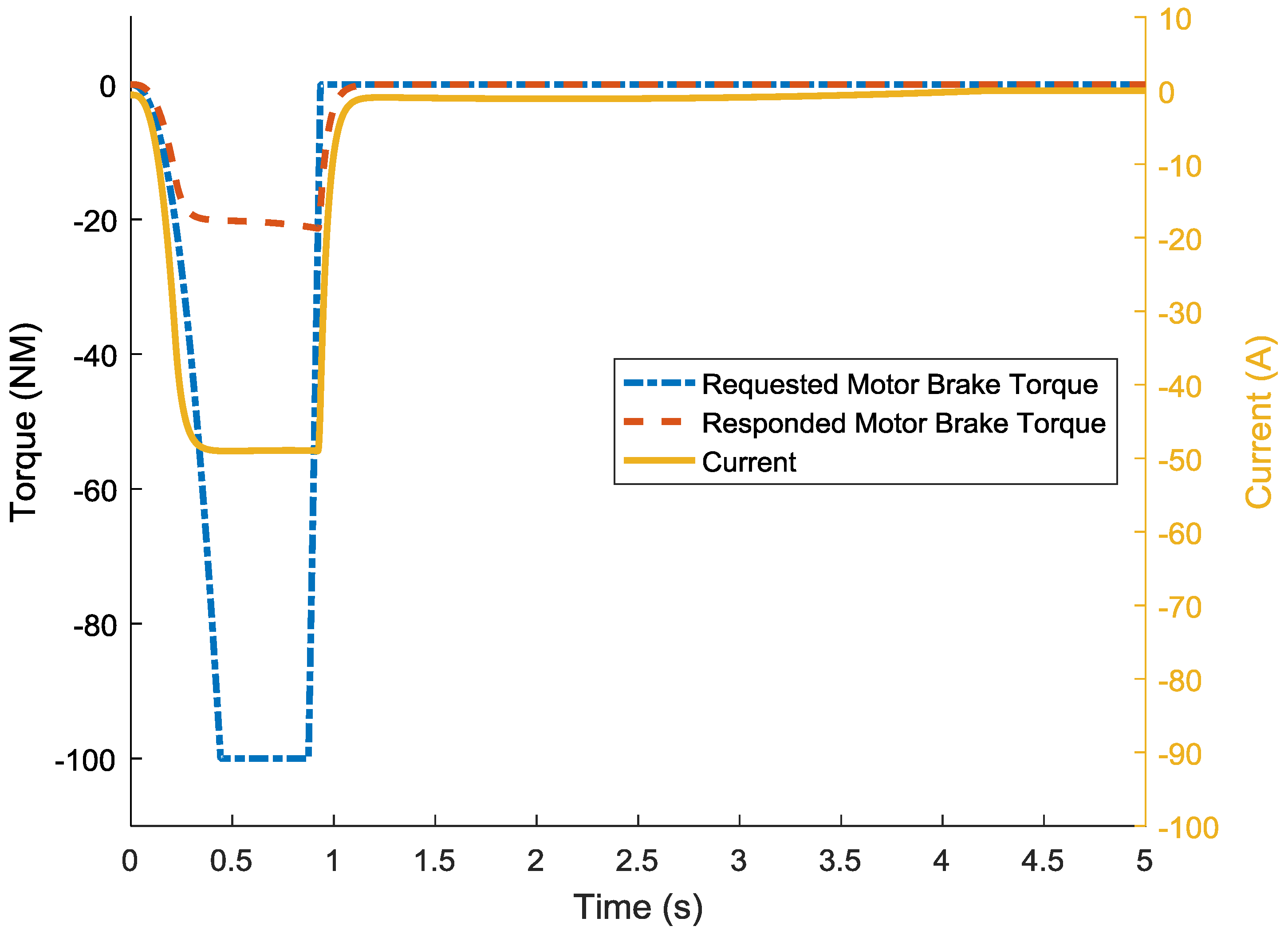
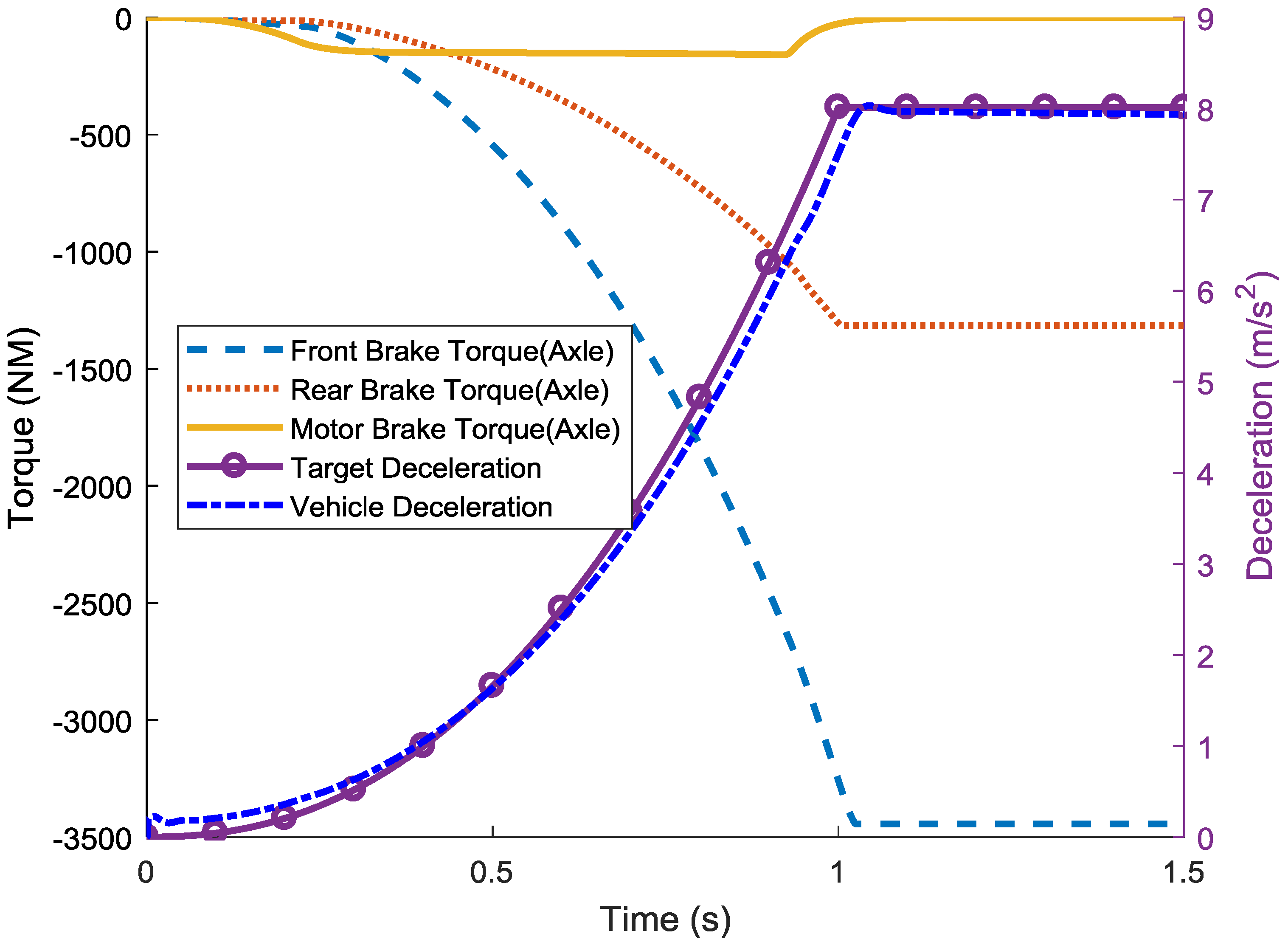
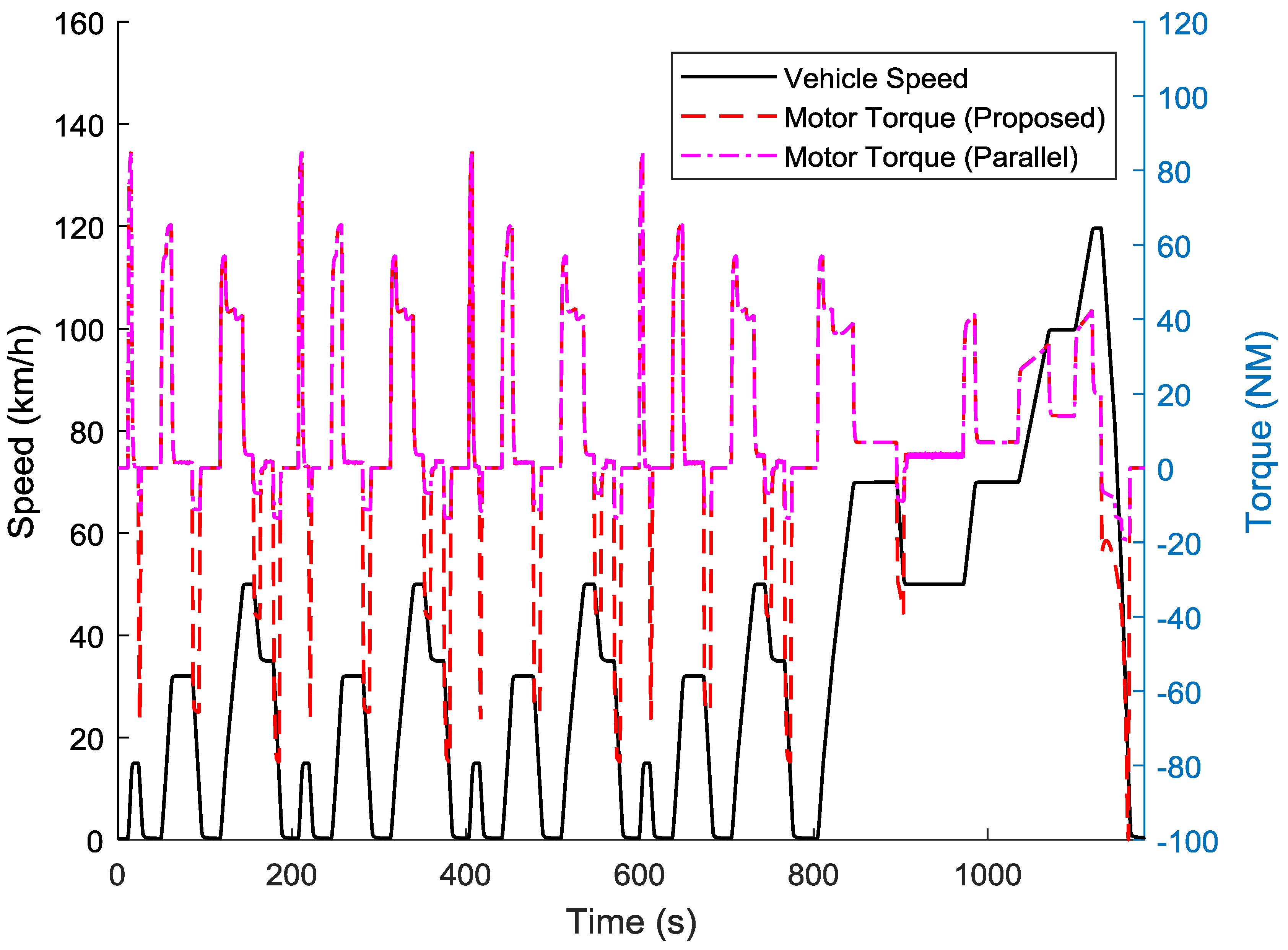
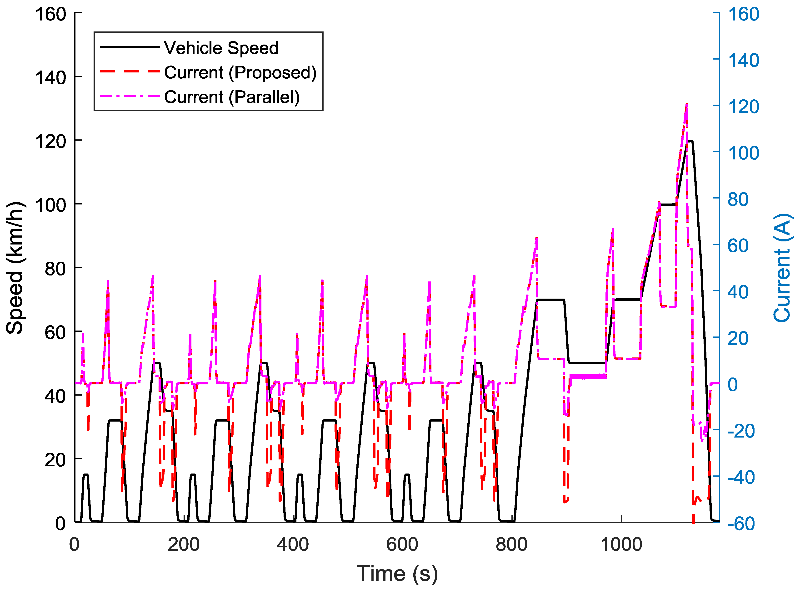
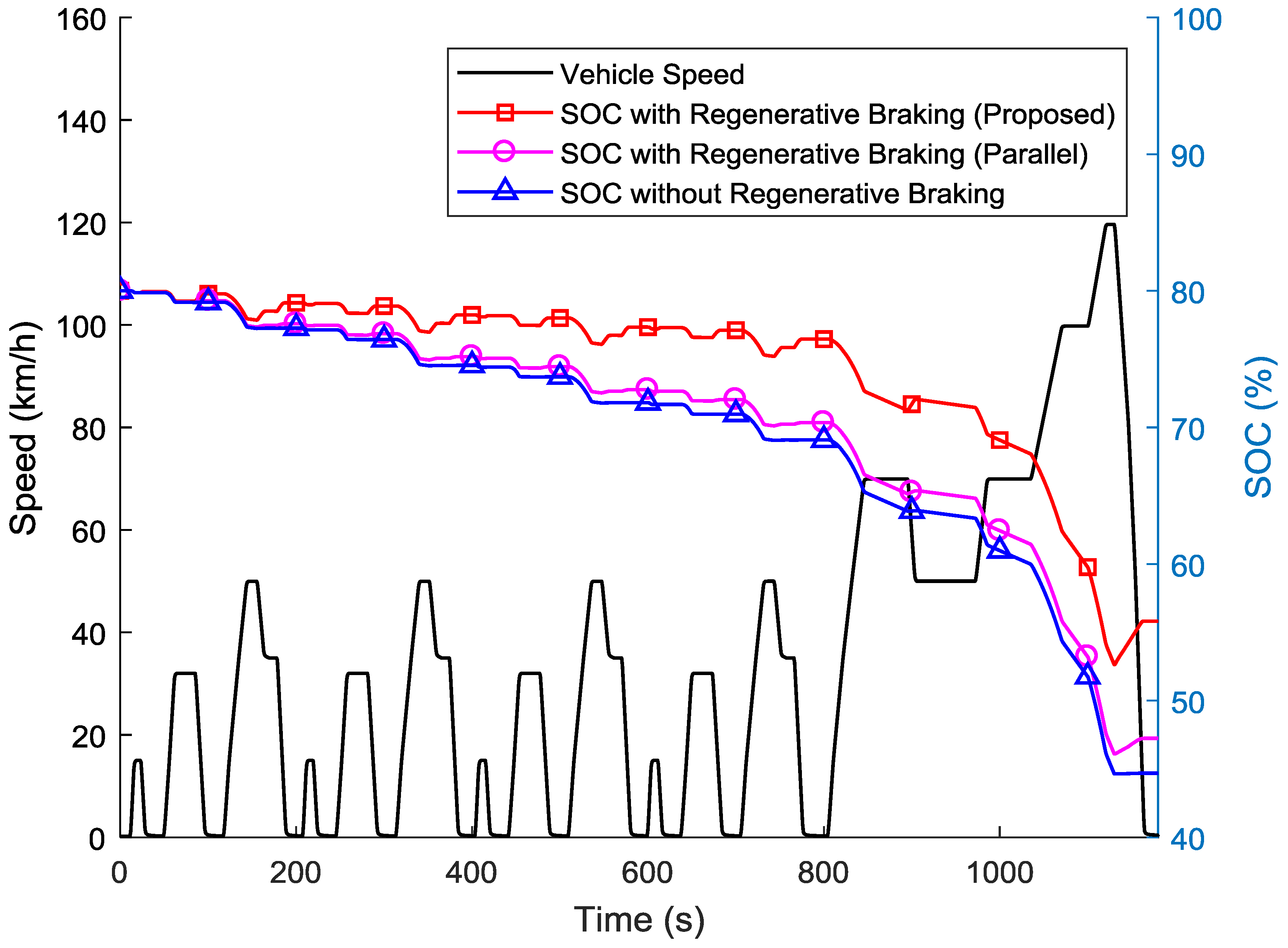
4.3. Simulation and Analysis of the System in Regenerative Braking Mode

With the regenerative braking function activated, the braking system will work in a more complicated mode. Figure 17, Figure 18 and Figure 19 show the simulation results of a regenerative braking process with constant braking rate. The measured brake force is shown in Figure 17 and it can be concluded that the brake force distribution algorithm was almost in line with expectations. However, the motor brake torque did not reduce to zero at once when the braking rate was beyond 0.7 g, which may cause the ABS function to not work properly. The delay was caused by the torque response characteristics of the motor and the brake force distribution strategy, which had a sudden change in motor torque at a high braking rate. In this simulation, the motor braking torque was much less than its upper limit due to its working condition. Figure 18 shows the change of brake force and deceleration in the first 1.5 s of the simulation, where it can be seen that as the motor braking force gradually reduced, the hydraulic braking force was compensated so that the deceleration could change with the target deceleration, however, there was still a small error between the actual vehicle deceleration and the target deceleration, partly because of the presence of air resistance, and also because the brake force distribution strategy is an open-loop strategy that does not have feedback correction on deceleration. Requested and responded motor torques, together with the current are shown in Figure 19, where we can see that the responded motor brake torque stopped following the requested torque at 0.4 s because the regenerative current nearly reached the limit of 50 A. As time progressed, the regenerative braking torque increased slightly due to a decrease of the speed while the current almost remained unchanged, this can be inferred from the characteristics of the motor, which is shown in Figure 8.

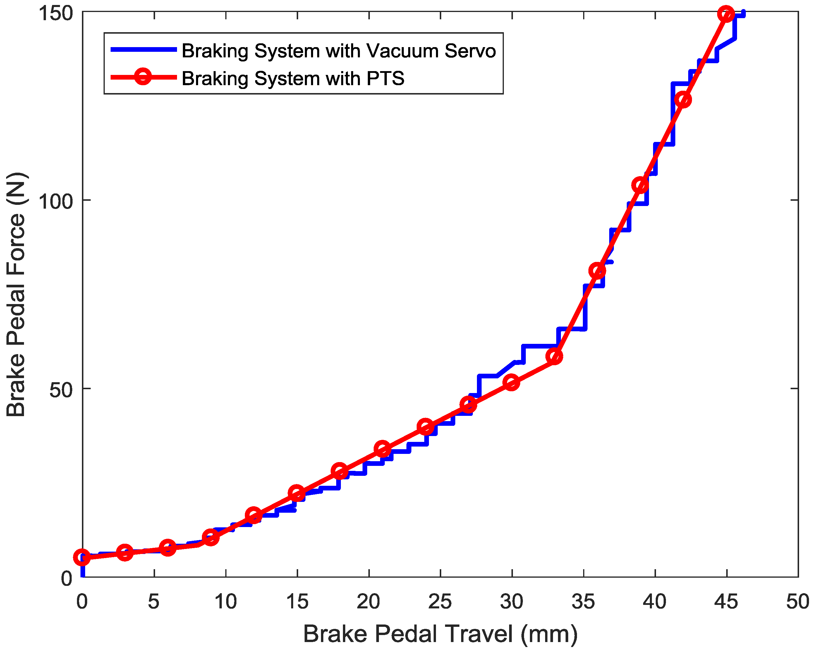
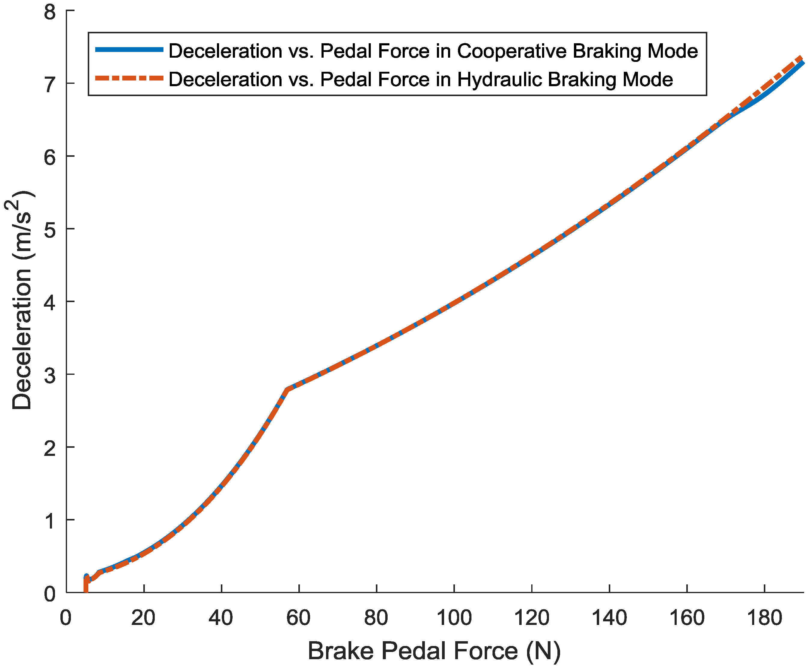
4.4. Simulation and Analysis of Brake Pedal Feel Simulation Mechanism

Through controlling the solenoid valves, we could connect the master cylinder to the pedal travel simulator to directly turn the hydraulic braking system into the pedal travel simulation mode and then input the pedal travel data into the model while collecting the pedal force data output from it. With the data collected, a pedal force vs. pedal travel curve that reflected the brake pedal feel characteristics was produced, as shown in Figure 20. This figure also shows the brake pedal force vs. travel data collected from a conventional hydraulic braking system with a vacuum booster. The simulation results showed that the pedal travel simulator could simulate the brake pedal feel to make the system feel like a conventional hydraulic braking system with vacuum booster.

The relationship between deceleration and brake pedal force is a basic and important factor for brake feel evaluation [24]. Simulations of the deceleration vs. brake pedal force characteristics were conducted and the results are shown in Figure 21. This characteristic was almost identical in the different working modes, with only a slight difference when the deceleration exceeded $6.5\mathrm{m}/{\mathrm{s}}^2$, therefore the difference was caused by the inaccurate estimation of brake force in the brake force distribution block.

4.5. Energy Recovery Performance Evaluation of the System in Simulation Environment

Simulations tests under New European Drive Cycle (NEDC) conditions with different brake force distribution strategies were carried out to evaluate the energy recovery performance of this system. The simulation results are shown in Figure 22, Figure 23 and Figure 24, which show variations of SOC, motor torque, and current on the DC bus under different cases, respectively. In Figure 22, the results showed that the strategy proposed in this paper could produce more motor braking torque than the parallel strategy. This means that the motor braking torque was utilized at a higher efficiency and outputted a higher current where more energy was recovered, as shown in Figure 23. The variation of SOC shown in Figure 24 indicated that after finishing an NEDC cycle, the SOC dropped from 80% to 55.83% under the proposed strategy. When compared to 47.24% under the parallel strategy and 44.70% under the hydraulic only strategy, the difference was 8.59% and 11.13%, respectively.

The comparison of SOC has already shown that the control strategy proposed in this paper could improve the efficiency of energy recovery, however, it can also be analyzed and evaluated in more detail. Lv’s paper proposed two evaluation indexes for the contribution of regenerative braking to energy efficiency improvement: contribution to the driving range extension of the vehicle, and contribution to the energy consumption reduction of the vehicle [25]. Since the energy consumption was much easier to calculate in this case, the latter index was used to evaluate the energy recovery performance. The contribution made by regenerative braking to energy consumption reduction was defined as [25]:

$${\delta }_E=\frac{E_{regen\_off}-E_{regen\_on}}{E_{regen\_off}}\times 100\%$$

(23)

where ${\delta }_E$ is the contribution ratio to energy consumption reduction; and $E_{regen\_on}$ and $E_{regen\_off}$ are the energy consumed with and without regenerative braking under a certain amount of driving range, respectively.

Energy efficiency and contribution to energy efficiency, which are calculated based on the simulation results, are shown in

Table 2. Comparison of energy recovery performance under different brake force distribution strategies.

Strategy	Energy Efficiency (kWh/100 km)	Contribution to Energy Efficiency Improvement (%)
Hydraulic only	12.5466	-
Parallel	11.6438	7.20
Proposed	8.5907	31.53

. Based on these results, it appears that the system and the control strategy proposed in this paper were able to recovery kinetic energy during braking more effectively than the traditional parallel distribution strategy.

5. Conclusions

In this paper, a regenerative braking system with a cooperative hydraulic braking system and pressure control methods, as well as the brake force distribution strategy were proposed. Then, the system and the electric vehicle platform were modeled, and several basic tests were simulated to evaluate the performance of the pedal feel simulation mechanism, the pressure control method, and the brake force distribution strategy. Finally, simulations under the NEDC driving cycles with different brake force distribution strategies were carried out and the energy recovery performance of the proposed system was evaluated by comparing the energy efficiency and contribution to energy efficiency improvement under different strategies. The simulations results showed the feasibility and effectiveness of the system proposed. In the future, the authors will focus on the integration of the stability control and regenerative braking control strategy, as well as the implementation of this system on electric cars driven by in-wheel hub motors.

References

1. Ma, H.; Balthasar, F.; Tait, N.; Riera-Palou, X.; Harrison, A. A new comparison between the life cycle greenhouse gas emissions of battery electric vehicles and internal combustion vehicles. Energy Policy 2012, 44, 160–173. [Google Scholar] [CrossRef]
2. Conti, R.; Galardi, E.; Meli, E.; Nocciolini, D.; Pugi, L.; Rindi, A. Energy and wear optimisation of train longitudinal dynamics and of traction and braking systems. Veh. Syst. Dyn. 2015, 53, 651–671. [Google Scholar] [CrossRef]
3. Pugi, L.; Malvezzi, M.; Papini, S.; Vettori, G. Design and preliminary validation of a tool for the simulation of train braking performance. J. Mod. Transp. 2013, 21, 247–257. [Google Scholar] [CrossRef]
4. Ganzel, B.J. Hydraulic Brake System with Controlled Boost. U.S. Patent 8,544,962, 29 October 2008. [Google Scholar]
5. Kim, S.M. Regenerative Brake Control Method. U.S. Patent 8,616,660, 11 May 2011. [Google Scholar]
6. Akita, K.; Yamamoto, T.; Miyazaki, T.; Uraoka, T.; Watanabe, K. Brake Control System. U.S. Patent 9,238,454, 4 February 2011. [Google Scholar]
7. Matsushita, S. Vehicle Braking Device. U.S. Patent 8,746,813, 6 May 2010. [Google Scholar]
8. Yang, Y.; Zou, J.; Yang, Y.; Qin, D. Design and simulation of pressure coordinated control system for hybrid vehicle regenerative braking system. J. Dyn. Syst. Meas. Control 2014, 136, 051019. [Google Scholar] [CrossRef]
9. Ko, J.; Ko, S.; Son, H.; Yoo, B.; Cheon, J.; Kim, H. Development of brake system and regenerative braking cooperative control algorithm for automatic-transmission-based hybrid electric vehicles. IEEE Trans. Veh. Technol. 2015, 64, 431–440. [Google Scholar] [CrossRef]
10. Wang, B.; Huang, X.; Wang, J.; Guo, X.; Zhu, X. A robust wheel slip ratio control design combining hydraulic and regenerative braking systems for in-wheel-motors-driven electric vehicles. J. Frankl. Inst. 2015, 352, 577–602. [Google Scholar] [CrossRef]
11. Zhang, J.; Lv, C.; Gou, J.; Kong, D. Cooperative control of regenerative braking and hydraulic braking of an electrified passenger car. Proc. Inst. Mech. Eng. Part D J. Automob. Eng. 2012, 226, 1289–1302. [Google Scholar] [CrossRef]
12. Huang, X.; Wang, J. Model predictive regenerative braking control for lightweight electric vehicles with in-wheel motors. Proc. Inst. Mech. Eng. Part D J. Automob. Eng. 2012, 226, 1220–1232. [Google Scholar] [CrossRef]
13. Guo, H.; He, H.; Xiao, X. A predictive distribution model for cooperative braking system of an electric vehicle. Math. Probl. Eng. 2014, 2014, 828269. [Google Scholar] [CrossRef]
14. Nian, X.; Peng, F.; Zhang, H. Regenerative braking system of electric vehicle driven by brushless DC motor. IEEE Trans. Ind. Electron. 2014, 61, 5798–5808. [Google Scholar] [CrossRef]
15. Pugi, L.; Grasso, F.; Pratesi, M.; Cipriani, M.; Bartolomei, A. Design and preliminary performance evaluation of a four wheeled vehicle with degraded adhesion conditions. Int. J. Electr. Hybrid Veh. 2017, 9, 1–32. [Google Scholar] [CrossRef]
16. Zhang, J.; Lv, C.; Qiu, M.; Li, Y.; Sun, D. Braking energy regeneration control of a fuel cell hybrid electric bus. Energy Convers. Manag. 2013, 76, 1117–1124. [Google Scholar] [CrossRef]
17. Kang, M.; Li, L.; Li, H.; Song, J.; Han, Z. Coordinated vehicle traction control based on engine torque and brake pressure under complicated road conditions. Veh. Syst. Dyn. 2012, 50, 1473–1494. [Google Scholar] [CrossRef]
18. Zhao, X.; Li, L.; Song, J.; Li, C.; Gao, X. Linear Control of Switching Valve in Vehicle Hydraulic Control Unit Based on Sensorless Solenoid Position Estimation. IEEE Trans. Ind. Electron. 2016, 63, 4073–4085. [Google Scholar] [CrossRef]
19. Lutsey, N.; Sperling, D. Energy efficiency, fuel economy, and policy implications. Transp. Res. Rec. J. Transp. Res. Board 2005, 1941, 8–17. [Google Scholar] [CrossRef]
20. Pacejka, H. Tire and Vehicle Dynamics; Elsevier: Amsterdam, The Netherlands, 2005. [Google Scholar]
21. Gu, J.; Ouyang, M.; Li, J.; Lu, D.; Fang, C.; Ma, Y. Driving and braking control of PM synchronous motor based on low-resolution hall sensor for battery electric vehicle. Chin. J. Mech. Eng. 2013, 26, 1–10. [Google Scholar] [CrossRef]
22. Yang, I.; Lee, W.; Hwang, I. A Model-Based Design Analysis of Hydraulic Braking System; 0148-7191; SAE International: Warrendale, PA, USA, 2003. [Google Scholar] [CrossRef]
23. Peng, D.; Zhang, Y.; Yin, C.-L.; Zhang, J.-W. Combined control of a regenerative braking and antilock braking system for hybrid electric vehicles. Int. J. Automot. Technol. 2008, 9, 749–757. [Google Scholar] [CrossRef]
24. Ebert, D.G.; Kaatz, R.A. Objective Characterization of Vehicle Brake Feel; 0148-7191; SAE International: Warrendale, PA, USA, 1994. [Google Scholar] [CrossRef]
25. Lv, C.; Zhang, J.; Li, Y.; Yuan, Y. Mechanism analysis and evaluation methodology of regenerative braking contribution to energy efficiency improvement of electrified vehicles. Energy Convers. Manag. 2015, 92, 469–482. [Google Scholar] [CrossRef]
Figure 1. Layout of the powertrain and cooperative braking system.
Energies 11 00378 g001
Figure 2. Layout of the hydraulic braking system.
Energies 11 00378 g002
Figure 3. Block diagram for cooperative braking controller.
Energies 11 00378 g003
Figure 4. Brake force distribution vs. braking rate.
Energies 11 00378 g004
Figure 5. Experimental data of the FCV characteristics test.
Energies 11 00378 g005
Figure 6. The equivalent structure of the hydraulic braking circuit.
Energies 11 00378 g006
Figure 7. Simulation platform layout.
Energies 11 00378 g007
Figure 8. Steady-state torque response of the electric motor.
Energies 11 00378 g008
Figure 9. Regenerative braking torque is limited when motor is running at low speed.
Energies 11 00378 g009
Figure 10. Pressure-volume characteristics of front and rear brake calipers. (a) Pressure-volume characteristics of the front brake caliper; (b) Pressure-volume characteristics of the rear brake caliper.
Energies 11 00378 g010
Figure 11. Sinusoidal response curve of front brake pressure.
Energies 11 00378 g011
Figure 12. Ramp response curve of front brake pressure.
Energies 11 00378 g012
Figure 13. Partial enlarged view of the pressure response curves with different pressure control method.
Energies 11 00378 g013
Figure 14. Pressure and valve control signals of the front left wheel.
Energies 11 00378 g014
Figure 15. Changes of vehicle speed and wheel speed in hydraulic braking only mode.
Energies 11 00378 g015
Figure 16. Measured brake force distribution in hydraulic braking only mode.
Energies 11 00378 g016
Figure 17. Measured brake force distribution in regenerative braking mode.
Energies 11 00378 g017
Figure 18. Change of brake force and deceleration during regenerative braking.
Energies 11 00378 g018
Figure 19. Change of motor torque and current during regenerative braking.
Energies 11 00378 g019
Figure 20. Test of brake pedal feel characteristics.
Energies 11 00378 g020
Figure 21. Deceleration vs. brake pedal force characteristics in different working modes.
Energies 11 00378 g021
Figure 22. Variation of motor torque in the New European Driving Cycle (NEDC) simulation with different brake force distribution strategies.
Energies 11 00378 g022
Figure 23. Variation of the current on the DC bus in the NEDC simulation with different brake force distribution strategies.
Energies 11 00378 g023
Figure 24. Variation of SOC in the NEDC simulation with different brake force distribution strategies.
Energies 11 00378 g024