Position Sensorless Control of Switched Reluctance Motor with Consideration of Magnetic Saturation Based on Phase-Inductance Intersection Points Information

Abstract

The precise estimation of position is an essential concern for the control of a switched reluctance motor (SRM). Given the prominent role of position, the promising sensorless control approach for an SRM drive should be capable of providing accurate position. An inductance-based approach has been widely applied in the position estimation. However, the estimated accuracy suffers from the magnetic saturation effect, resulting in the poor performance of sensorless operation. This paper presents a reversible synchronization of commutation with the corresponding rotor position for SRM. With the consideration of magnetic saturation, the proposed approach is taken as a suitable candidate and plays an essential role in accommodating the requirement of optimal control. The relationship between a typical inductance position and magnetic circuit saturation is investigated. The instant of the intersections is sensed by comparing the instantaneous inductance of adjacent phases. Thus, the predicted position is obtained with the information of the special point and the calculated average speed. Compared with other existing methods, the proposed approach has the certain advantages, such as the ability to update the estimated speed and position six times per electrical period, which guarantees the estimated accuracy. The proposed approach is also valid even when the motor is operated at an acceleration state and heavy load operation. In addition, the requirement of the educated inductance structure is not unnecessary, less memory space is needed in the chip, and the accumulated error is eliminated. The simulation and experimental findings demonstrate the feasibility and practicality of the proposed position estimation approach with carrying out the inertial operation, load mutation, and high-speed test.

1. Introduction

Switched reluctance motor (SRM) is widely used due to its inherent features, such as high efficiency, robust structure, and fault tolerance [1,2,3]. Unlike permanent-magnet synchronous motors, a rotor structure has no windings and permanent magnets. Hence, the motor is a potential candidate for high-temperature motor control and possesses the potential for the application in the electric vehicles [4,5,6]. Encoders, resolvers, and hall-effect sensors are widely employed to obtain the accurate rotor angle. However, a few problems, such as low reliability and susceptibility to interference, accompany such applications. Sensorless control approach is the useful solution. An modifications of the sensorless scheme is made to get a high accuracy estimation for four-quadrant operation [7].

A discrete-time sliding mode observer for the sensorless vector control of permanent magnet synchronous machine is proposed in Reference [8]. Reference [9] gives an overview on sensorless control strategies using very nice technical language and context. In the problem of the sensorless control, an important aspect is the disturbance rejection that generates inaccuracies in the controlled variables. To estimate an external inaccessible disturbance, an extended Kalman filter is designed in Reference [10].

The nonlinear characterization makes it a more challenging issue for switched reluctance machines in terms of the position estimation [11]. Various sensorless strategies, such as inductance profile based [4], observe based approach [5], and an intelligent algorithm-based approach [6] have been presented to eliminate the sensors. The categorical methods will be introduced in the following content. A few control-based approaches for SRM drive systems are demonstrated to eliminate the position sensors. In Reference [11], it is found that position estimation inaccuracy is very vulnerable to the saturation when SRM is operated under heavy load conditions. The influence of measurement error intensity is minimized with an automatic adaptation characteristic. Other control-based approaches are established to achieve a high position accuracy. Voltage-pulse-injection-based methods are widely employed in the sensorless position estimation for low speed or standstill conditions. However, as the speed increases, there is little interval and space available for the injection, resulting in less pulses injected into the idle phase. In that case, the position information is hard to extract. To overcome this problem, a single pulse injection method is proposed in Reference [12]. Compared with traditional injection method, fewer pulses are demanded in the approach. Besides, a 3-D-lookup table is adopted to demonstrate the relationship between the integrator and the position. Thus, the injection method is extended to the high-speed operation region. With improved pulse injection, the operated condition is improved and suitable for both low-speed and high-speed range conditions. However, the redefined table will increase the burden of storage for the controller. Another current gradient sensorless method employed for high-speed operation has been reported in Reference [13], which makes it possible that the motor is able to be operated at high-speed SRM with 100,000 rev/min. The parameter variations, such as change in DC-link voltage, are also analyzed to examine the stability of the system. However, additional hardware is required for the detection for the current gradient sensorless (GGS) peak.

The observed hall signal is sensed and the machine can be operated with accurate position estimation. However, the low-resolution hall signals are the primary obstacle for the low speed operation. An accurate position is estimated by applying a phase inductance vector coordinate transformation and phase current slope difference method in Reference [14]. Both a coordinate transformation and phase current slope difference method are combined and the position is obtained by the alpha-beta transformation, and the heave-load condition is discussed to prove the effectiveness. Nevertheless, the coordinate transformation increases the computational complexity. Several intelligent algorithm methods have also been reported to obtain the position in previous research. Two networks are trained separately [15], one for a low-speed condition and the other is for a high-speed condition. In this method, the control parameters are recreated. Although the approach is suitable for the whole-speed range operation, the estimated accuracy is dependent on the neuron number. The accuracy can be promoted with the increasing of the neuron number; however, the computation burden also increases. High computation stress will make it impossible to implement the arithmetic in the low-performance controller. An improved neural network is described in Reference [16], in which the computational burden is able to be reduced by 77%. Although high estimated accuracy is obtained, this neural network method is unsuitable for high-speed condition due to its time-consuming calculation. A neuro-fuzzy learning system is investigated in Reference [17] where the reference current and conducting phase voltage are completely utilized. Experiment result shows that the motor is operated well by using the corresponding speed and rotor position. An observer-based method is generally suitable for the high-speed condition. To accommodate operation at a wider range of speeds, a hybrid sensorless control approach is presented in Reference [18]. Initially, the low-resolution sensor is used for low speed or standstill operation. As the speed increases, it is switched to a sliding mode observer-based estimation scheme. The performance of the motor will be degraded in the case of the inaccuracy installation. Numerous studies focus on extracting the position from the phase inductance or flux linkage information [19,20,21,22]. Unlike previous studies, Reference [7] proposed an entire-speed-range sensorless strategy with structure modifications. The wide speed range running ability means the system can accommodate the application requirement. The relationship between rotor position, phase current, and the incremental is investigated in Reference [23]. The position information is precisely proven without the implementation requirement of large memory space or extra hardware. However, the challenge is that the position estimated accuracy is prone to be affected by a variety of factors, such as mutual flux and magnetic saturation, which is brought about via the inductance-based method. To minimize the effects of the mutual flux, the mutual flux is fully investigated in Reference [24]. The exciting mode where the mutual flux does not exist is selected.

The magnetic saturation is taken into consideration in the sensorless control in Reference [25]. The rotor position varies with the phase inductance. The phase inductance is calculated using the gradient of the flux linkage. However, the magnetization inductance curve is necessary to be stored in the Digital Signal Processor (DSP) and takes up a lot of memory. Based on former studies, this paper proposes an estimated position approach by utilizing six typical points. The contribution of this paper is that it provides a solution for precise estimation with the consideration of magnetic saturation. The specific advantages are shown as follows.

We try to make the difference and contribution clear. The instant of the intersections is sensed by comparing the instantaneous inductance of adjacent phases. Thus, the predicted position is obtained with the information of the special point and the calculated average speed. In addition, the requirement of the inductance structure is not demanded. In addition, the estimated speed and position are insensitive to magnetic saturation, to overcome the problem that the position estimation is vulnerable to be affected by the inductance saturation, the estimated speed and estimated angle are able to be updated six times per electrical period, in which the saturation effect is taken into consideration. Moreover, the accumulative error for a period can be eliminated. Simulation and experiment results show that the performance of the sensorless scheme using six update points is superior to that of conventional method.

The organization of this paper is demonstrated as follows. In Section 2, the principle of the phase inductance estimation is discussed. In Section 3, the proposed position sensorless control strategy based on special position is described in detail. Section 4 and Section 5 prove the simulation and experimental results, respectively. Finally, conclusions are given in Section 6.

2. Phase Inductance Estimation Principle

Three-phase SRM inductance information has the characteristics of symmetry and periodicity, and inductance varies periodically as the rotor position changes.

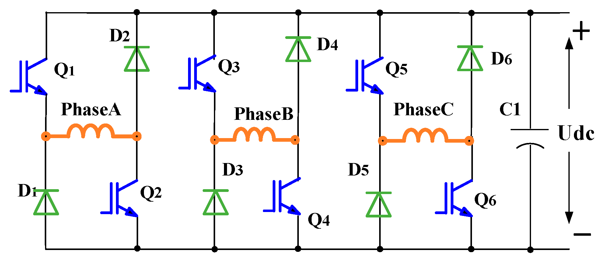
To obtain the inductance profile, high-frequency pulse-voltage is generally exerted on the non-conducting phase windings. In the conducting phase, the full-cycle inductance information is extracted from the responding excitation current. A 12/8 three-phase switched reluctance motor is taken as an example in this study, and a three-phase asymmetric half-bridge prototype power converter is utilized. The topology of three-phase asymmetric half-bridge power converter is shown in Figure 1.

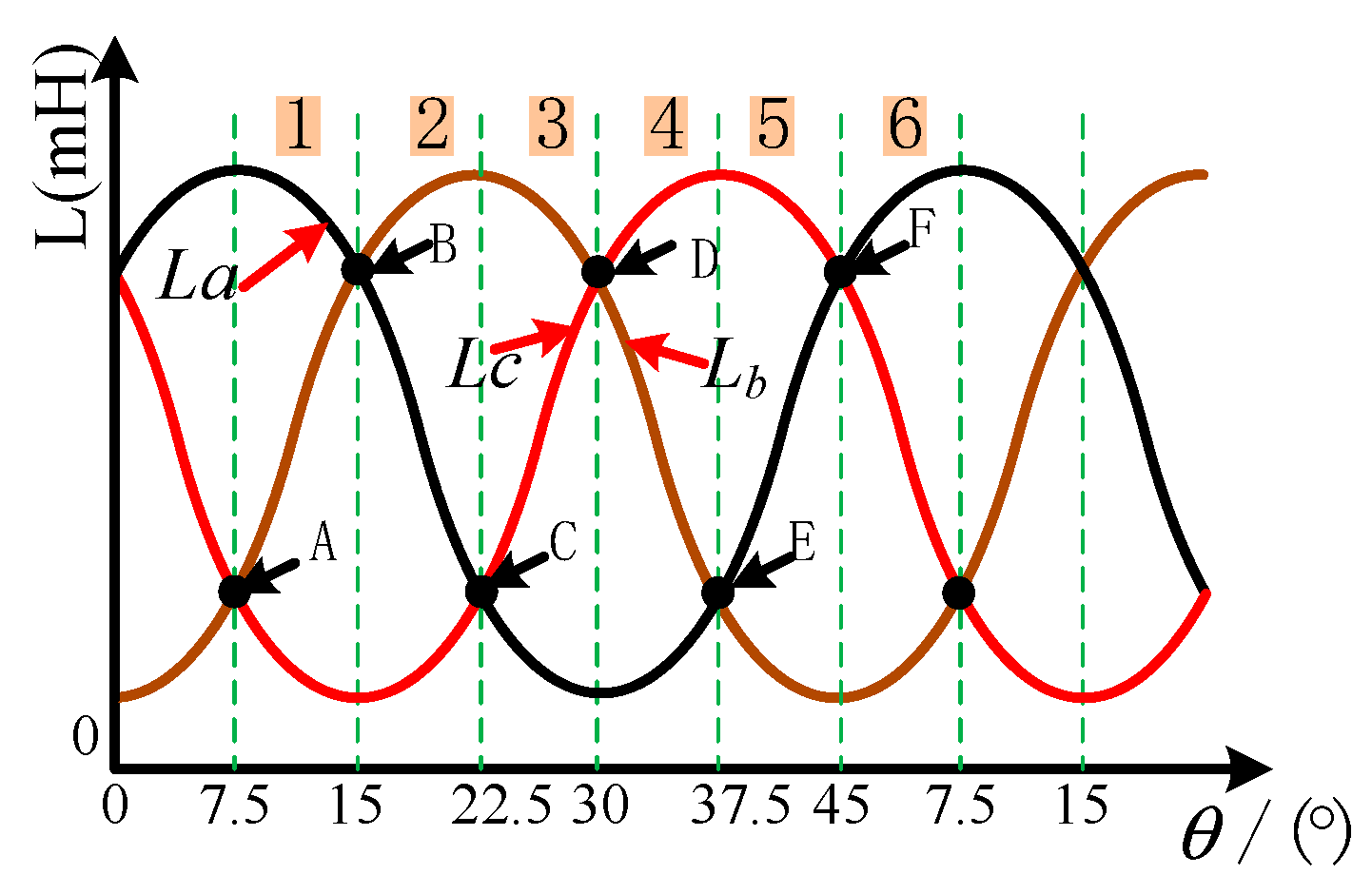
The topology of the control system has the following features. A total of six inductance intersections are available during a 360° electrical cycle. Furthermore, the electrical angle interval between the adjacent inductance profile intersections is 60° and the corresponding mechanical angle is 7.5°. The phase inductance varying with the rotor position is shown in Figure 2, in which the magnetic circuit saturation is not considered. The stator salient pole and the center of the rotor groove are aligned at 0° position, and the stator salient pole and the center of the rotor salient pole are aligned at 22.5° (mechanical angle) position. In addition, it should be noted that the position of the intersections for adjacent inductance is evidently specific and fixed. Moreover, the speed and position estimation is able to be achieved by using the six typical intersection positions.

The SRM phase voltage is expressed as follows:

$$V=iR+\frac{\partial \psi \left(\theta ,i\right)}{dt}$$

(1)

SRM has a nonlinear mapping relationship among flux linkage, position, and current. The partial derivatives are given by

$$V=iR+\frac{\partial \psi (\theta ,i)}{dt}|\begin{array}{l}\\ \theta =fixed\end{array}+\frac{\partial \psi \left(\theta ,i\right)}{dt}|\begin{array}{l}\\ i=fixed\end{array}$$

(2)

The k-phase represents the conducting phase, and the k − 1 phase is the non-conducting phase. Considering the influence of k − 1 phase mutual inductance, the k-phase flux linkage can be expressed as

$${\psi }_k=L_{k,k}{i}_k+M_{k,k-1}{i}_{k-1}$$

(3)

where $L_{k,k}$ is the k-phase self-inductance, and $M_{k,k-1}$ is the mutual inductance between the k-phase and the k − 1 phase.

Then, the k-phase voltage equation can be expressed as:

$$\begin{array}{l}{V}_k=i_{k}R+\frac{d{L}_{k,k}(\theta ,i)}{d{i}_k}\cdot \frac{d{i}_k}{dt}\cdot i_k+\frac{d{L}_{k,k}(\theta ,i)}{d\theta }\cdot \frac{d\theta }{dt}\cdot i_k+L_{k,k}(\theta ,i)\cdot \frac{di}{dt}+\frac{d{M}_{k,k}}{d\theta }\cdot \frac{d\theta }{dt}\cdot i_k\\ +\frac{d{M}_{k,k-1}}{d{i}_{k-1}}\cdot \frac{d{i}_{k-1}}{dt}\cdot i_{k-1}+\frac{d{M}_{k,k-1}}{d{i}_k}\cdot \frac{d{i}_k}{dt}\cdot i_{k-1}+M_{k,k-1}\frac{d{i}_{k-1}}{dt}\end{array}$$

(4)

The k − 1 phase flux linkage is given as:

$${\psi }_{k-1}=M_{k,k-1}{i}_k+L_{k,k-1}{i}_{k-1}$$

(5)

The k − 1 phase voltage equation can then be given as:

$$V_{k-1}=i_{k-1}R+\frac{d{L}_{k-1,k-1}}{d\theta }\cdot \frac{d\theta }{dt}\cdot i_{k-1}+\frac{d{L}_{k-1,k-1}}{d{i}_{k-1}}\cdot \frac{d{i}_{k-1}}{dt}\cdot i_{k-1}+L_{k-1,k-1}\cdot \frac{d{i}_{k-1}}{dt}+\frac{d{M}_{k-1,k}}{d\theta }\cdot \frac{d\theta }{dt}\cdot i_k+\frac{d{M}_{k-1,}k}{d{i}_k}\cdot \frac{d{i}_k}{dt}\cdot i_k+\frac{d{M}_{k-1,k}}{d{i}_{k-1}}\cdot \frac{d{i}_{k-1}}{dt}\cdot i_k+M_{k-1}^{}\cdot k\cdot \frac{d{i}_k}{dt}$$

(6)

The k-phase voltage expression can be simplified to:

$$V_k=R{i}_k+L_{inck}\frac{d{i}_k}{dt}+M_{inck}\frac{d{i}_{k-1}}{dt}+w_m(\frac{d{L}_{kk}}{d\theta }\cdot i_k+\frac{d{M}_{k,k-1}}{d\theta }\cdot i_{k-1})$$

(7)

where the k-phase incremental inductance $L_{inck}$ can be obtained using Equation (8), k-phase incremental mutual inductance $M_{inck}$ can be obtained using Equation (9), and $w_m$ is the angle velocity:

$$L_{inck}=\frac{d{L}_{kk}}{d{i}_k}\cdot i_k+L_{kk}+\frac{d{M}_{k,k-1}}{d{i}_k}\cdot i_{k-1}$$

(8)

$$M_{inck}=\frac{d{M}_{k,k-1}}{d{i}_{k-1}}\cdot i_{k-1}+M_{k,k-1}$$

(9)

The k − 1 phase voltage expression can be simplified to:

$$V_{k-1}=R{i}_{k-1}+L_{inck-1}\frac{d{i}_{k-1}}{dt}+M_{inck-1}\frac{d{i}_k}{dt}+w_m(\frac{d{L}_{k-1,k-1}}{d\theta }\cdot i_{k-1}+\frac{d{M}_{k,k-1}}{d\theta }\cdot i_k)$$

(10)

where the k − 1 phase incremental inductance $L_{inck-1}$ can be obtained using Equation (11), and the k − 1 phase incremental mutual inductance $M_{inck-1}$ can be obtained using Equation (12):

$$L_{inck-1}=\frac{d{L}_{k-1,k-1}}{d{i}_{k-1}}\cdot i_{k-1}+L_{k-1,k-1}+\frac{d{M}_{k,k-1}}{d{i}_{k-1}}\cdot i_k$$

(11)

$$M_{inck-1}=\frac{d{M}_{k,k-1}}{d{i}_k}\cdot i_k+M_{k,k-1}$$

(12)

3. Proposed Position Sensorless Control Strategy Based on Special Position

3.1. Inductance Calculation on Line

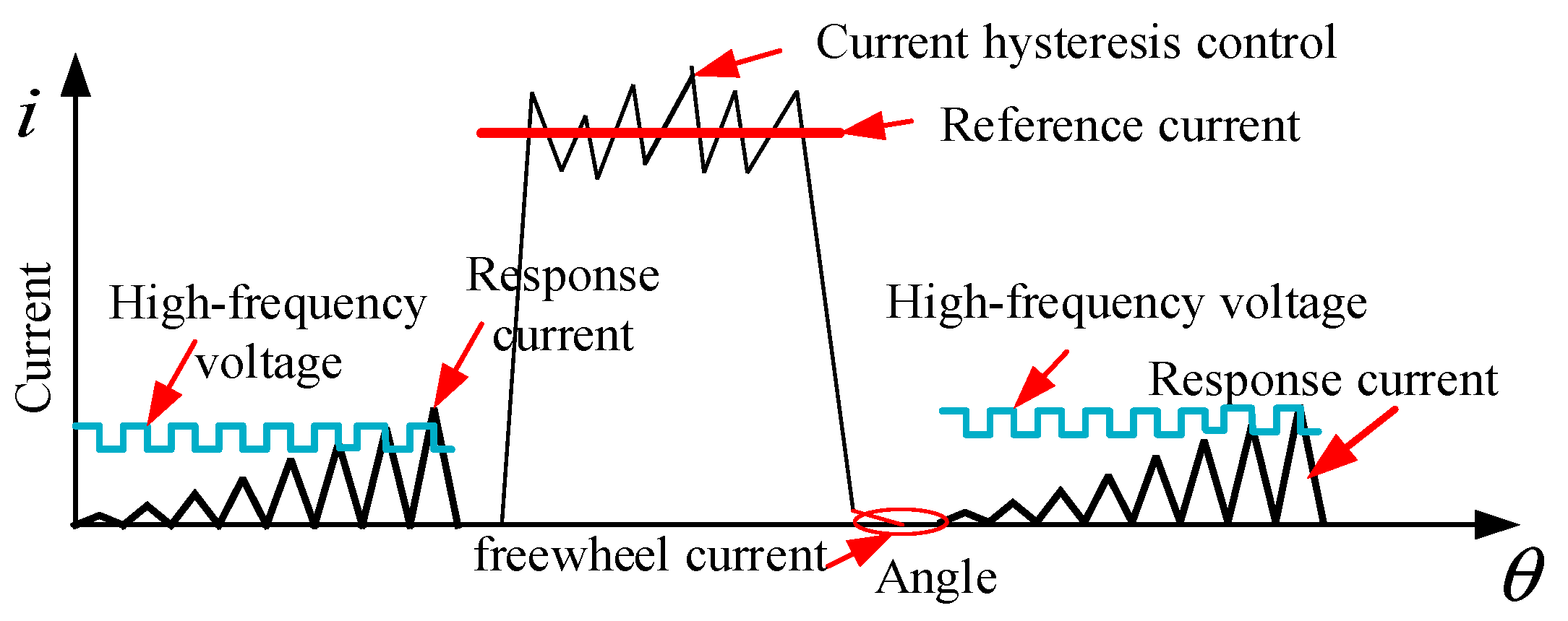
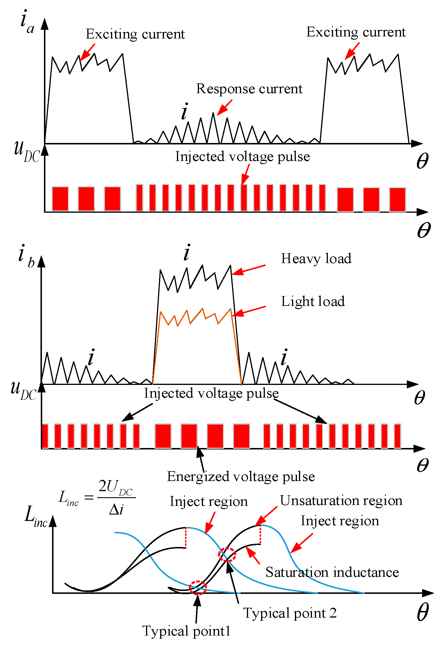
As shown in Figure 3, the hysteresis current control is adopted in the conducting phase, simultaneously, using a series of high-frequency voltage pulse injections are exerted on the non-conducting phase windings. The rising and falling slopes of its response current varies periodically according to the rotor position. The inductance information can be extracted by measuring the changing slope of current at a fixed control cycle. The inductance estimation process is described as follows.

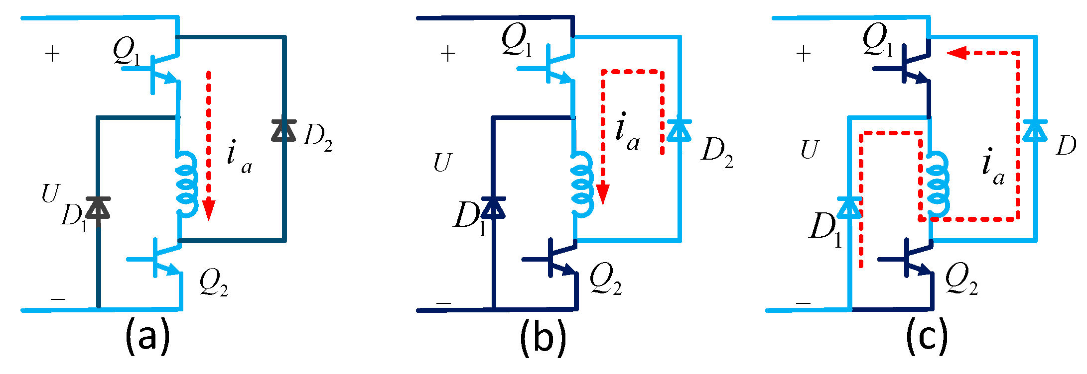
The state of corresponding phase is defined as conductive when the switching devices Q₁ and Q₂ are turned on. Consequently, positive voltage is applied to the winding terminal, as shown in Figure 4a. The voltage drop at the diodes and power switches is negligible. Thus, the voltage expression is shown in Equation (13). Two current-reflowing modes exist when one switching device of a phase is turned off. One is the current reflowing through diode D₂ and switching device Q₁ when Q₂ is turned off; in this state, there is no voltage applied on the windings, as shown in Figure 4b, and the voltage expression is expressed in Equation (14). The other one is current reflowing to the power supply through diode D₁ and D₂ when switching devices Q₁ and Q₂ are turned off; in this state, the negative voltage is applied on the winding terminal, as shown in Figure 4c. The current of the negative voltage exerted mode rapidly decreases compared with that of the natural freewheeling mode. The negative voltage combing freewheeling mode is adopted in this study. The detailed state of the switching device and the terminal voltage are shown in

Table 1. State of working phase and idle phase.

Device	Working State	State	Terminal Voltage
Q1, Q2	Energized mode	0	Udc
D1, D2	Demagnetization mode	0	−Udc
Q2, D1	Freewheeling mode	0	0
Q1, Q2	Idle state	1	Udc
Q3, Q4	Energized mode	0	Udc
D3, D4	Demagnetization mode	0	−Udc
Q4, D4	Freewheeling mode	0	0
Q3, Q4	Idle state	1	Udc
Q5, Q6	Energized mode	0	Udc
D5, D6	Demagnetization mode	0	−Udc
Q6, D6	Freewheeling mode	0	0
Q5, Q6	Idle state	1	Udc

.

$$U_{DC}=R{i}_k+L_{inck}\frac{d{i}_{k\_on}}{dt}+M_{inck}\frac{d{i}_{k-1\_on}}{dt}+w_m(\frac{d{L}_{k,k}}{d\theta }\cdot i_k+\frac{d{M}_{k,k-1}}{d\theta }\cdot i_{k-1})$$

(13)

$$0=R{i}_k+L_{inck}\frac{d{i}_{k\_on}}{dt}+M_{inck}\frac{d{i}_{k-1\_on}}{dt}+w_m(\frac{d{L}_{k,k}}{d\theta }\cdot i_k+\frac{d{M}_{k,k-1}}{d\theta }\cdot i_{k-1})$$

(14)

$$-U_{DC}=R{i}_k+L_{inck}\frac{d{i}_{k\_off}}{dt}+M_{inck}\frac{d{i}_{k\_off}}{dt}+w_m(\frac{d{L}_{k,k}}{d\theta }\cdot i_k+\frac{d{M}_{k,k-1}}{d\theta }\cdot i_{k-1})$$

(15)

Equation (16) can be obtained after Equations (14) and (16) are subtracted:

$$L_{inck}=\frac{2U_{DC}-M_{inck}(\frac{d{i}_{k-1\_off}}{dt}-\frac{d{i}_{k-1\_on}}{dt})}{\frac{d{i}_{k\_on}}{dt}-\frac{d{i}_{k\_off}}{dt}}$$

(16)

In the absence of mutual inductance between phases, the incremental inductance can be rewritten as

$$L_{inck}=\frac{2U_{dc}}{\frac{d{i}_{k\_on}}{dt}-\frac{d{i}_{k\_off}}{dt}}$$

(17)

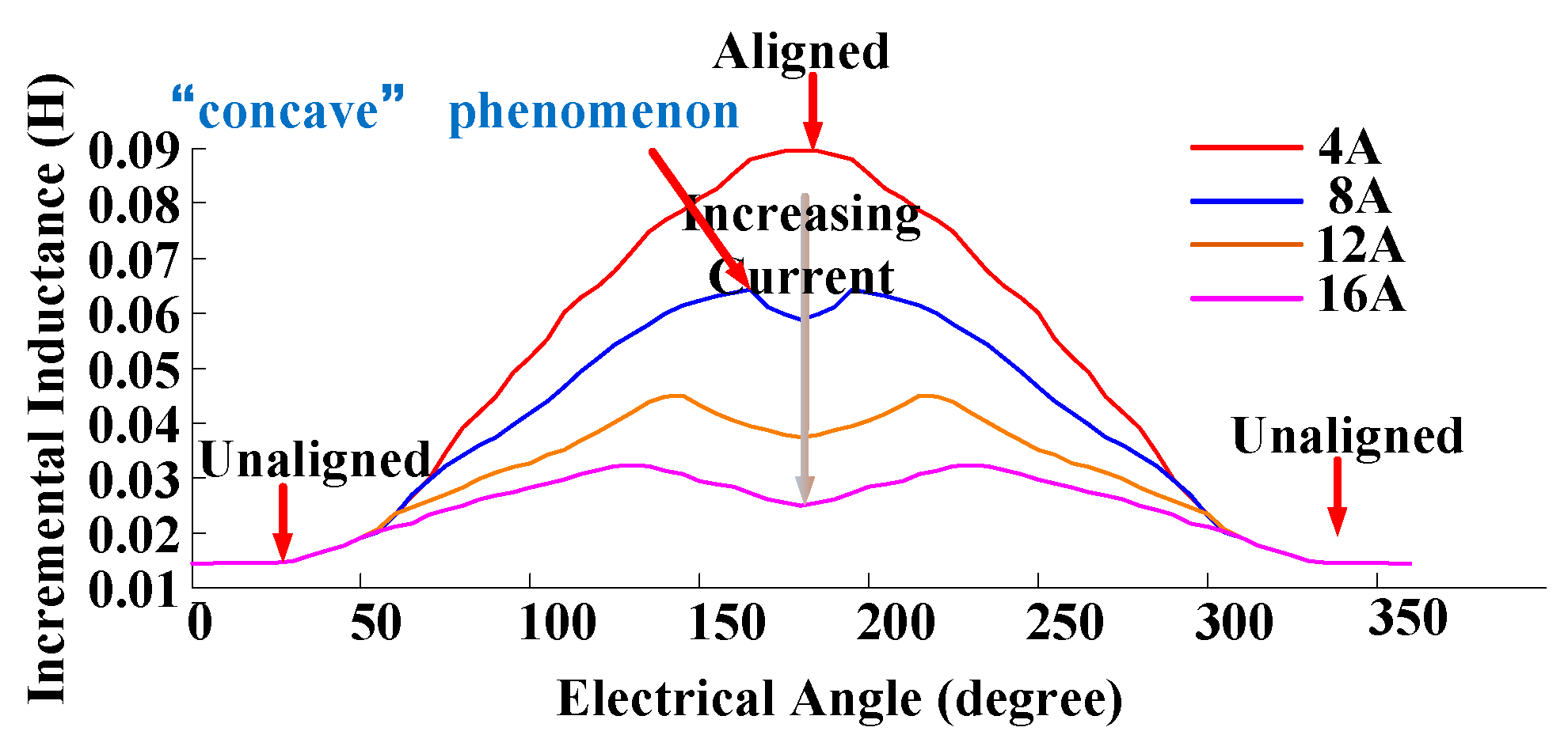
Notably, the incremental inductance is related to the current changing rate and bus voltage according to Equation (17). The influence of back electromotive force (EMF) and the winding voltage drop can be eliminated in accordance with the slope difference method, and the sensitivity of speed in the inductance estimation process is reduced. Apparently, the incremental inductance curve demonstrates a “concave” phenomenon when the current increases, as described in Figure 5. The incremental inductance is non-monotonous with angle. Consequently, the relationship between incremental inductance information and position is not a one-to-one correspondence; therefore, further obtaining the inductance value is necessary.

According to Equations (8) and (17), the inductance can be further expressed as:

$$L_{kk}=L_{inck}-\frac{d{L}_{kk}}{d{i}_k}\cdot i_k$$

(18)

The magnetic saturation is supposed to be neglected when the motor is operated at light load and in inertia mode. The inductance curves are most coincident in this condition, and a mapping relationship exists between inductance and position. A considerable difference is observed when the current increases and the motor is running in the magnetic saturation region. Moreover, the relationship between inductance and position no longer shows a one-to-one correspondence. Thus, reconsidering the typical intersection position of inductance is necessary.

3.2. Typical Position Point Selection under Magnetic Saturation Operation

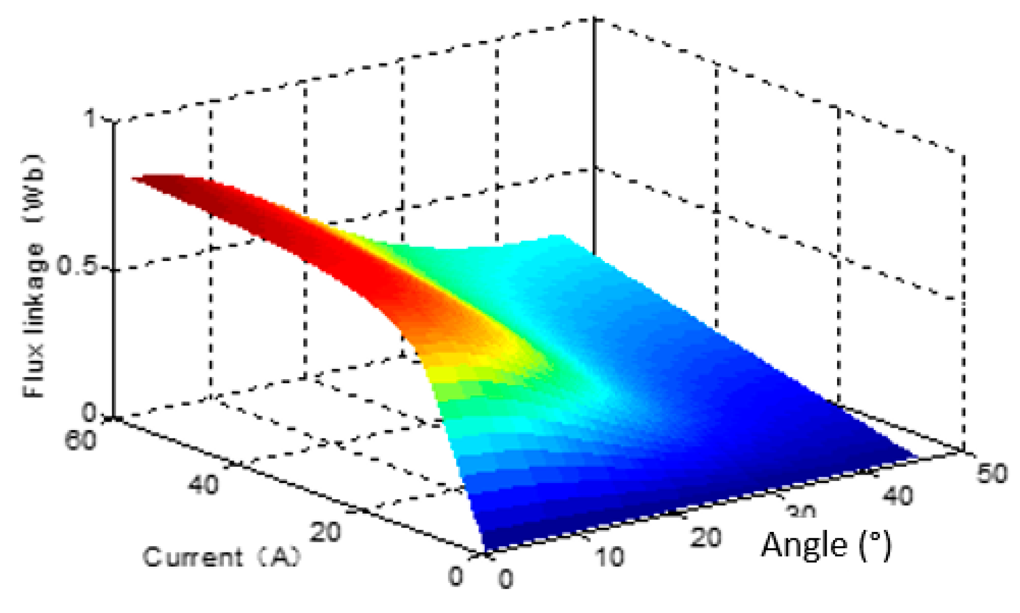
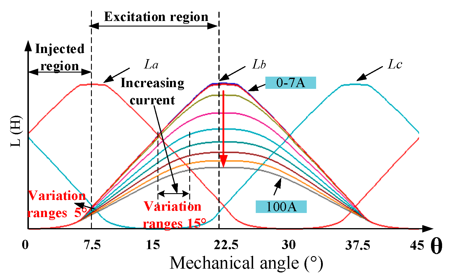
The magnetic circuit will be gradually saturated as the load current increases, as shown in Figure 6, the linear relationship between the flux linkage and current is not suitable anymore and the “concave” phenomenon will appear at the inductance curve. Traditionally, operating the motor in the magnetic circuit saturation state is an excellent choice to obtain a large torque. The low-inductance region is defined, and its range is approximately within 0–15°. As indicated in Figure 7, the inductance curve profile is nearly in agreement under different saturated currents. Furthermore, the magnetic saturation effect on the inductance intersection is negligible, and the maximum intersection position under different saturated currents is supposed to be within 2°. The speed and angle estimations can only be updated twice by employing the intersection in the low-inductance area, which leads to the low resolution for the estimated position. On the basis of the preceding analysis, the typical intersection position of the low-inductance region can be an output position point for position estimation due to its insensitivity to current. In the case of conducting phase B, a single inductance curve intersection exists between non-conducting and conducting phase B in the low-inductance region during a 360° electrical cycle. The situation is relatively different for high-inductance regions. The intersection position is remarkably affected by magnetic saturation, with the intersection position bias even reaching 15° (electrical angle). Obviously, the fixed intersection position in the high-inductance area should not be directly used.

As mentioned above, the intersections at the high-inductance area accompanying with that of the low-inductance are selected as the update points for position estimation in this study to improve position estimation accuracy. A total of six update points are available per 360° electrical period, which is three times greater than the traditional method. The relationship between the load saturation current and intersection point position is investigated by determining the intersection characteristic of the inductance curve. The rotor speed and position are eventually estimated by utilizing the six inductance intersections.

3.3. Estimation of Speed and Position under Driving Mode

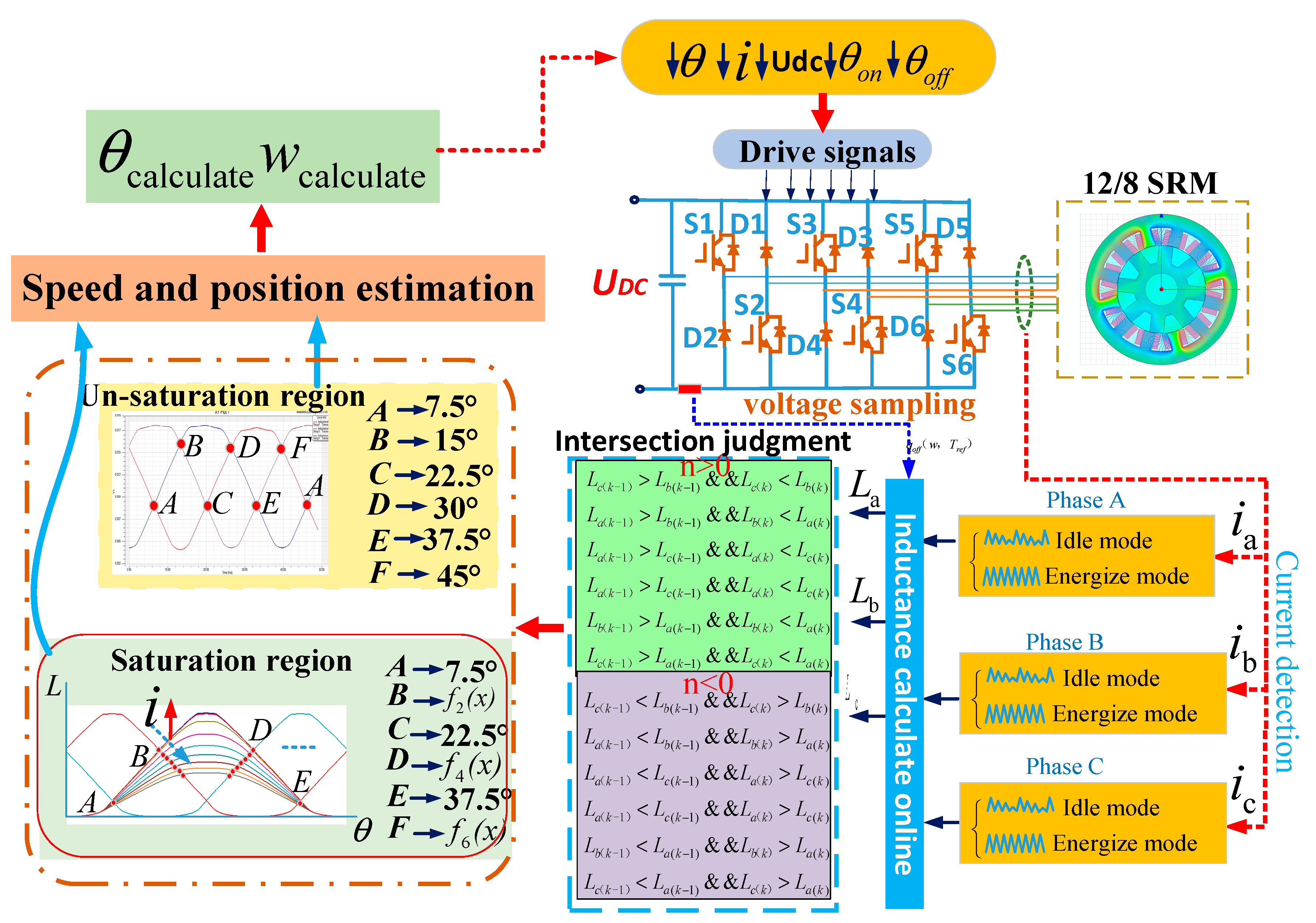
A typical block diagram of position sensorless control system for SRM based on the typical point is shown in Figure 8. The commutation controller is responsible for generating gate signals for the power devices. Speed and position are estimated based on the intersection position information and the interval. In the proposed method, hysteresis control is adopted by taking advantage of the sampling current and speed controller output. A deviation exists between the estimated and given speeds. The compensated partial mismatch is then transmitted to controlled speed as the reference value of the current loop.

Commutation is an important requirement in the process of SRM operation. Accurate inductance online identification and realization of position estimation are keys to accurate motor commutation. Inductance identification includes driving and idle-phase inductance identification. The values of bus voltage $U_{DC}$ and phase currents $i_a,i_b,i_c$, are measured through the voltage sampling circuit and the high accuracy current sensors, respectively. At the same time, analog-to-digital converters are responsible for the identification. The incremental inductance is first calculated using Equation (18). Subsequently, the full-cycle inductance is further deduced by using Equation (19).

The nonlinear mapping relationship between inductance and angle is obtained through curve fitting or Fourier decomposition after obtaining the cycle inductance value. Existing viable solutions on the comprehensive relationship of the inductance and the position result in a complex structure, thereby impeding their industrial application. Two segments are regarded as effective solutions in this paper, where one is that the intersection position at low inductance is fixed whenever the motor is running at magnetic saturation or not. The other is that the intersection position at high inductance varies with the saturation current. The recognition of the relationship between intersection position and saturation current is needed. The intersection position at the low inductance region can be directly obtained synchronously with the function of the current and the inductance intersection position in the high-inductance region by offline processing is obtained. Finally, six intersection positions are available for the estimation. A schematic of inductance estimation during motor operation in the driving mode is given in Figure 9. The inductance of the conducting phase is calculated online by using hysteresis control of the phase current information. In addition, the inductance of the non-conducting phase is calculated by utilizing the current response information obtained from the high-frequency voltage pulse injection.

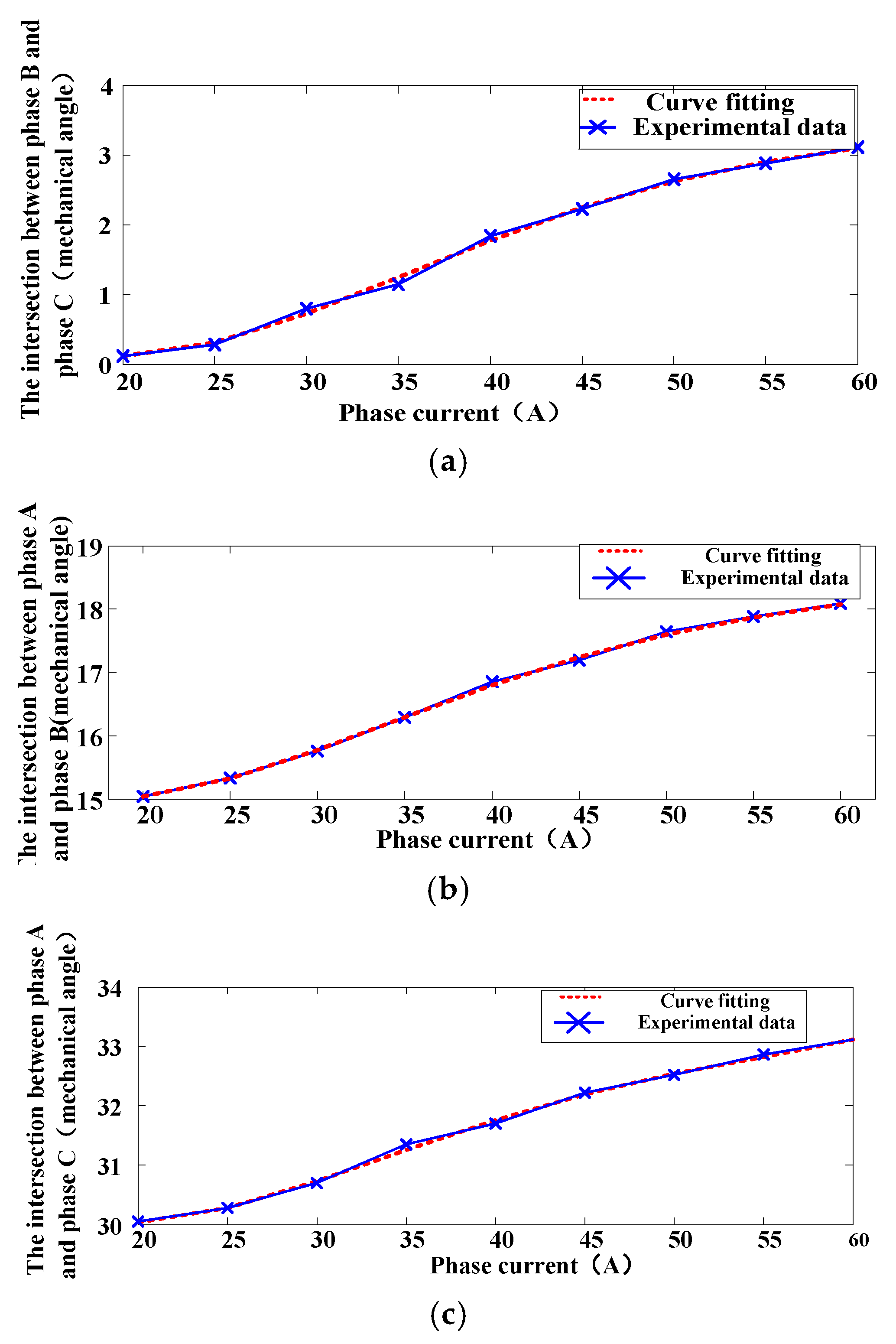
Figure 10a–c shows that the angle of inductance intersections in the low-inductance area is close to 7.5°, 22.5°, and 37.5°, respectively. The angle of inductance intersections in the high-inductance area changes significantly with saturation current, as shown in Figure 11a–c. The maximum position error can exceed 15° (electrical angle), and the output position angle of intersection points must be modified according to the current value.

The polynomial fitting mathematical expression is established to describe the relationship between the saturation current and the intersection position:

$$y=a_1{x}^5+a_2{x}^4+a_3{x}^3+a_4{x}^2+a_{5}x+a_6$$

(19)

Given the Digital Signal Processor (DSP) operation speed and positive correlation between fitting accuracy and fitting number, five polynomial fittings are properly selected in this study to meet the fitting accuracy. The fitting coefficients are shown in

Table 2. Polynomial fitting coefficients of angle and current.

Coefficient Parameters	Fitting Coefficient Inductance Intersection Phase A and B	Fitting Coefficient Inductance Intersection Phase A and C	Fitting Coefficient Inductance Intersection Phase C and B
$a_1$	2.02 × 10−6	1.692 × 10−6	2.615 × 10−6
$a_2$	−0.0003914	−0.0003226	−0.0004636
$a_3$	0.02635	0.02119	0.02902
$a_4$	−0.6446	−0.4833	−0.6709
$a_5$	5.278	18.54	35.14

.

It should be noted that the accuracy of Equation (19) is dependent on the fitting coefficient of the polynomial. However, the higher the accuracy, the more the fitting coefficient is demanded, which accompanies enhancing the complexity of the calculation. The intersection position under different saturation currents will be significant, but the variation tendency has certain rules. As the load current becomes larger, the intersection of the inductance “moves backward”. The more collection points of offline experiments, the more accurate the relationship between the position of the intersection and the current; conversely, low resolution is obtained with the rare acquisition points. Generally, the collection points are selected based on the rated current. In this paper, 5–10 point acquisitions are appropriate, and the position between the two points will not vary too much. Assuming that the rated current is 60 A, 0–10 A is the non-saturation zone, and 10–60 A is the saturation zone. The selection of offline measurement data at 10 A, 20 A, 30 A, 40 A, 50 A, and 60 A is appropriate; thus, the accuracy of the fitting is able to be achieved and guaranteed. With the low number of measurement points, the workload is able to be reduced.

The identification of the inductance intersection in the driving mode is similar to that of inertial operation, as shown in

Table 3. Inductance logic and special location point at saturated current.

Relationship of Adjacent Inductance Profiles (n > 0)	Relationship of Adjacent Inductance Profiles (n < 0)	Intersection	Typical Position
$\begin{array}{l}{L}_{c(k-1)}>L_{b(k-1)}\&\&L_{c\left(k\right)}<L_{b(k)}\\ L_{a(k-1)}>L_{b(k-1)}\&\&L_{b\left(k\right)}<L_{a(k)}\\ L_{a(k-1)}>L_{c(k-1)}\&\&L_{a\left(k\right)}<L_{c(k)}\\ L_{a(k-1)}>L_{c(k-1)}\&\&L_{a\left(k\right)}<L_{c(k)}\\ L_{b(k-1)}>L_{a(k-1)}\&\&L_{b\left(k\right)}<L_{a(k)}\\ L_{c(k-1)}>L_{a(k-1)}\&\&L_{c\left(k\right)}<L_{a(k)}\end{array}$	$\begin{array}{l}{L}_{c(k-1)}<L_{b(k-1)}\&\&L_{c\left(k\right)}>L_{b(k)}\\ L_{a(k-1)}<L_{b(k-1)}\&\&L_{b\left(k\right)}>L_{a(k)}\\ L_{a(k-1)}<L_{c(k-1)}\&\&L_{a\left(k\right)}>L_{c(k)}\\ L_{a(k-1)}<L_{c(k-1)}\&\&L_{a\left(k\right)}>L_{c(k)}\\ L_{b(k-1)}<L_{a(k-1)}\&\&L_{b\left(k\right)}>L_{a(k)}\\ L_{c(k-1)}<L_{a(k-1)}\&\&L_{c\left(k\right)}>L_{a(k)}\end{array}$	A	7.5°
		B	${\theta }_2=f\left(i_2\right)$
		C	22.5°
		D	${\theta }_4=f\left(i_4\right)$
		E	37.5°
		F	${\theta }_6=f\left(i_6\right)$

. The apparent distinction lies in the intersection position in the high-inductance area, which is calculated according to the polynomial fitting mathematical formula and cannot be separated from the real-time sampling current.

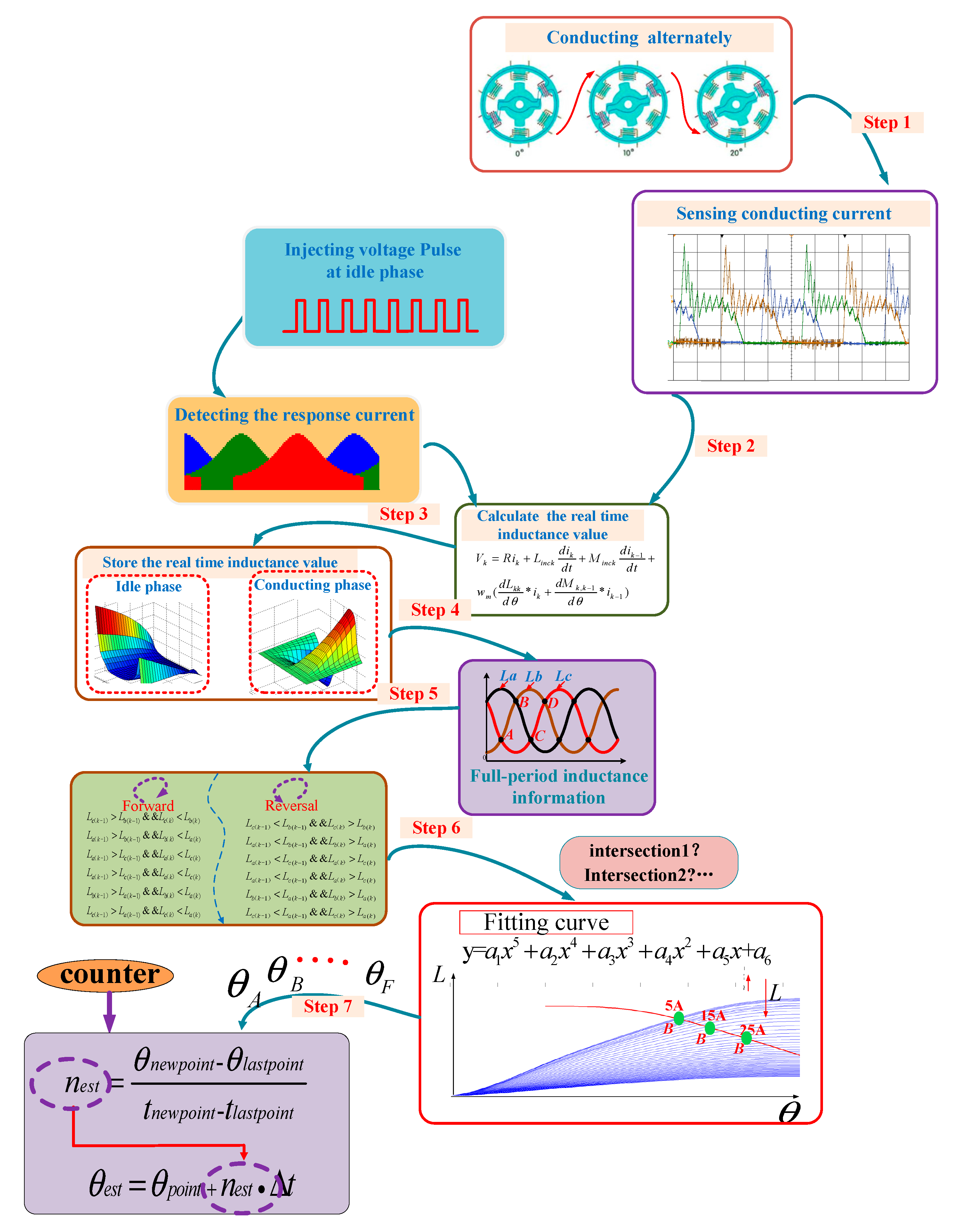
The flowchart of the estimation arithmetic is demonstrated in Figure 12. The rotor movement through two position points is relatively short under high speed operation, and the average speed between the update position points is considered constant. The motor rotor position estimation at the instant ${\theta }_{est}$ is then rewritten in Equation (20) as follows:

$${\theta }_{est}={\theta }_k+{\displaystyle \int \begin{array}{c}{t}_1\\ t_2\end{array}}\frac{\Delta \theta }{\Delta t_k}dt$$

(20)

where ${\theta }_k$ represents the rotor update position point; Δθ stands for the partial angle spacing between adjacent typical intersection point, which is considered a constant value 7.5°; $\Delta t_k$ denotes the rotor rotation time from one typical position to the other; $t_k$ stands for the k_th moment of updated point; and $t_1$ denotes any moment when the rotor rotates between two typical points, where the related equations are revealed in

Table 4. Speed and position estimation at the saturation current.

Intersection	Angular Speed Estimation	Position Estimation
Intersection 1 to Intersection 2	$w_{12}=\frac{f(i_2)-7.5}{T_{12}}$	$\theta =7.5+w_{12}t$
Intersection 2 to Intersection 3	$w_{23}=\frac{22.5-f(i_2)}{T_{23}}$	$\theta =f(i_2)+w_{23}t$
Intersection 3 to Intersection 4	$w_{34}=\frac{f(i_4)-22.5}{T_{34}}$	$\theta =f(i_2)+w_{23}t$
Intersection 4 to Intersection 5	$w_{45}=\frac{37.5-f(i_4)}{T_{45}}$	$\theta =f(i_4)+w_{45}t$
Intersection 5 to Intersection 6	$w_{56}=\frac{f(i_6)-37.5}{T_{56}}$	$\theta =37.5+w_{56}t$
Intersection 6 to Intersection 1	$w_{61}=\frac{(45-f(i_6))+7.5}{T_{61}}$	$\theta <45 \theta =f(i_6)+w_{61}t$
		$\theta >45 \theta =w_{61}t$

.

Where w₁₂, w₂₃, w₃₄, w₄₅, w₅₆, and w₁₆, represent the estimated angular velocity between different intersections; T₁₂, T₂₃, T₃₄, T₄₅, T₁₂, T₁₂, T₅₆, and T₆₁ stand for the interval when the rotor rotates from one intersection to the other; and t denotes the random instant when the rotor rotates between two adjacent intersections. It should be indicated that the proposed method is also effective for other structure motor and it is able to be extended for an n-phase SRM. The number of the special points depends on the stator poles and rotor poles. Supposing the construction of the SRM is n-stator poles and m-rotor poles, the conducting region should be defined as 360/m and there are 6n update points in total per revolution.

It is clear that the estimation accuracy will be promoted with the increasing phases and rotor poles.

4. Simulation Analysis

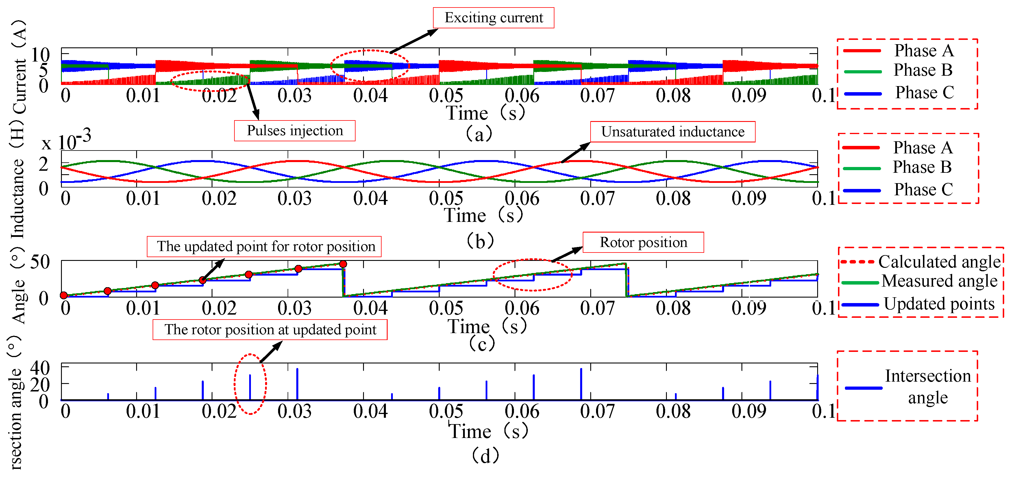
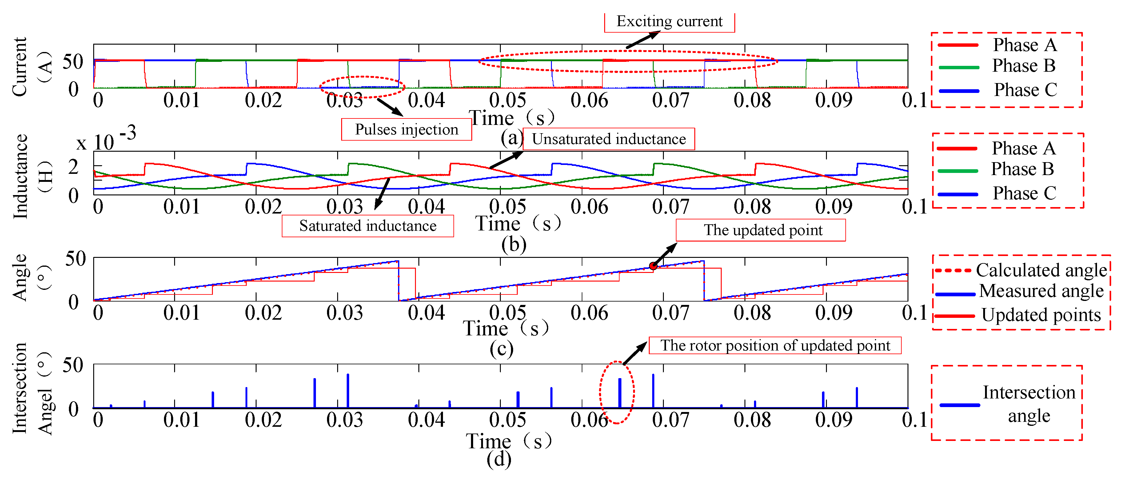
A 12/8 SRM simulation model is established in this paper. A series of voltage pulses were injected to the non-conducting phase, while simultaneously, the hysteresis control with a given 6 A current was utilized in the conducting phase. Figure 13 shows the estimated waveforms of the current, inductance, and position in the condition that the motor runs at a given current of 6 A. The curves indicate that three-phase inductances of the conducting and non-conducting phases were consistent. Similar to the inertia-operated state, the intersection positions were 7.57°, 15.04°, 22.55°, 30.07°, 37.51°, and 44.97°, respectively, approaching to the ideal defined values 7.5°, 15°, 22.5°, 30°, 37.5°, and 45°. The error between the predictive and actual positions was below 0.2°, which guaranteed the satisfactory performance of the motor drive system.

The given current value was set to 50 A to make the motor run in a magnetic saturation state, verifying the functionality of the proposed position estimation and its suitability for that state. As shown in Figure 14, the intersection positions in the low-inductance area were located at 7.41°, 22.42°, and 37.42°, which is similar to the preceding case. In the high-inductance area, the inductance intersection of the non-conducting phase and the conducting phase was obtained, and the position at the intersection point was calculated through the fitting formula. The simulation results show that the three intersection positions at the high-inductance area were nearly 15.05°, 30.08°, and 0.14° in the non-magnetic saturation operation state. As the motor ran in the magnetic saturation state, these aforementioned positions moved to 16.85°, 31.08°, and 1.84°, greater than the estimation value. The maximum deviation was close to 2°, which amounts to the electrical angle of 16°. The discrepancy will be further extended if the phase current continues to increase and the saturation is further intensified. With the proposed method, the extreme error of the estimated position was 1.1°, which was insensitive to the saturation effect.

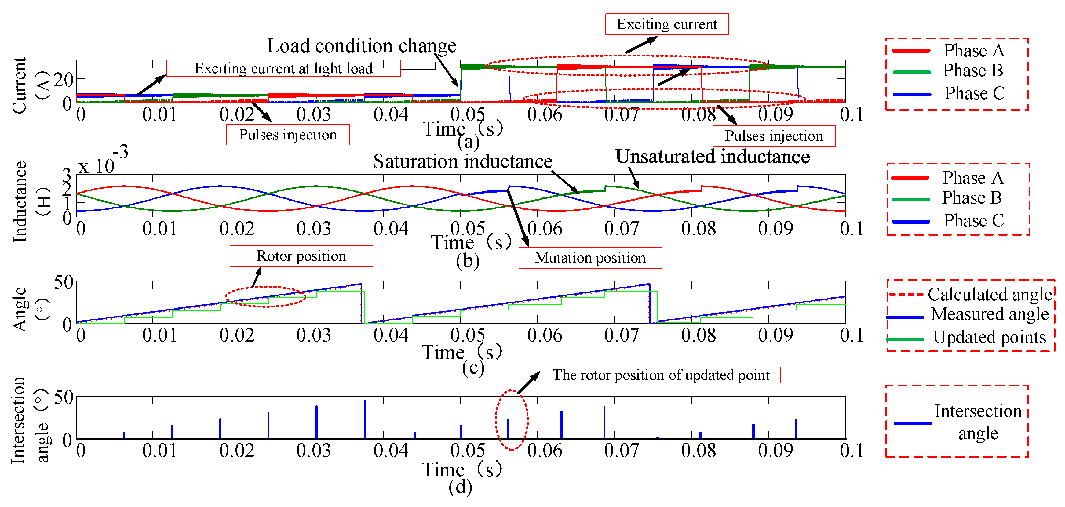
In order to simulate the load mutation, the given current increased from 10 A to 35 A. The simulation waveforms of the phase current, inductance, and estimated position are shown in Figure 15. The inductance curve distortion occurred when the current mutated, eventually returning to normal. The position estimation was unaffected by the inductance distortion since the update point remains uninterrupted. Notably, the estimated angle matches the actual angle well, and the error was under 1.2°. The demonstrated results verify the effectiveness of the proposed method for load mutation.

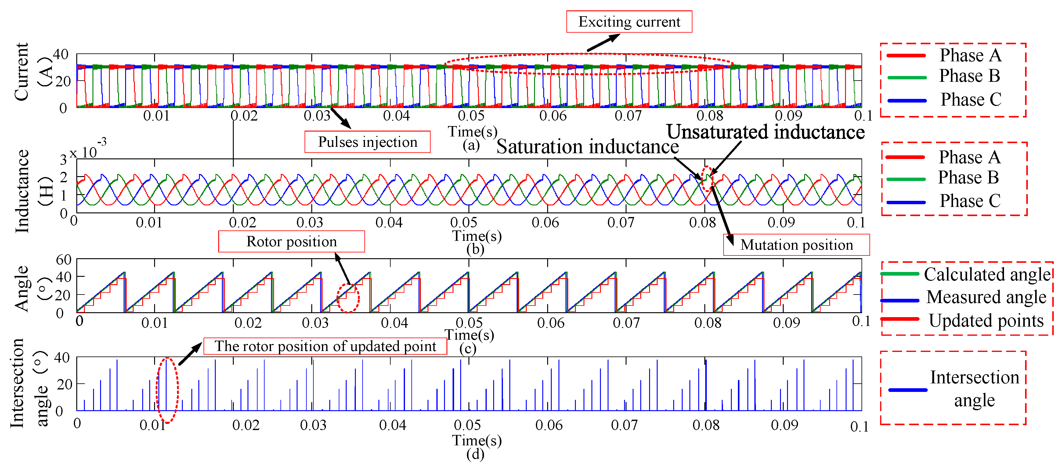
The simulation diagram of high-speed estimation is explored and presented in Figure 16. The motor is rapidly accelerated from a still state to 1200 rev/min when the given current is set to 30 A and maintained a steady-state speed operation. Simulation results reveal that the position estimation accuracy was approximately lower than that at low speed. The delay of the sampling instant was the main affecting factor. However, the maximum error did not exceed 1.5°. Evidently, the position estimation accuracy could also be ensured at high speed.

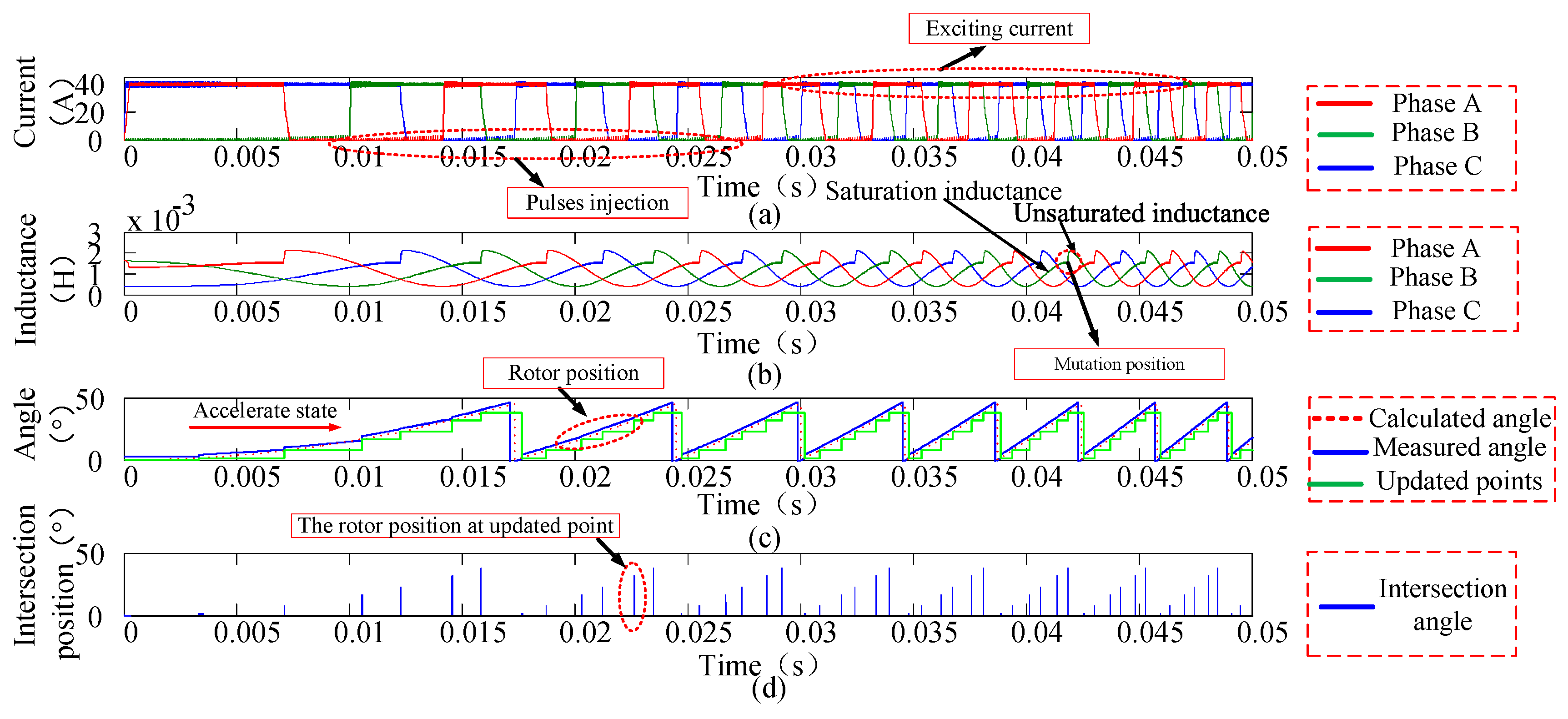
Following this, the acceleration simulation was performed, as exhibited in Figure 17. The speed evidently responds with an issued forward command and reaches the reference value within a short interval. The predictive speed between the two updated points was constant at a high–middle speed; thus, the estimated speed could track the actual speed by using the piecewise step method. However, the status was slightly different for low or varied speed operation since the average speed calculated in the previous interval was adapted to estimate the position of the present interval, inevitably leading to a deviation. Position estimation was evidently affected in the case of variable speed, especially when the speed change was relatively large. The present results show that the maximum position estimation error was able to reach 2.1°.

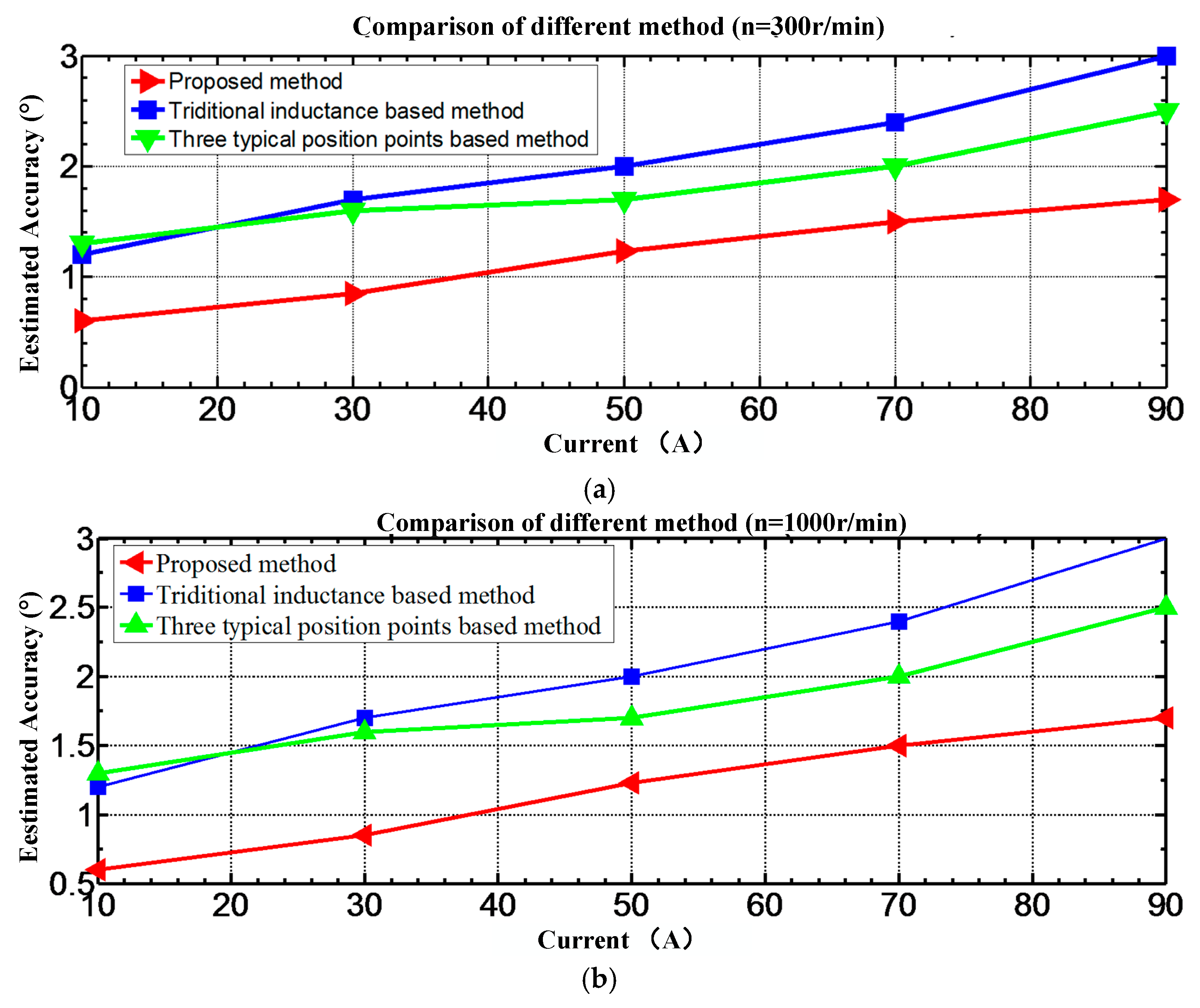
A different method containing the proposed approach, a traditional inductance-based method, and three typical position points-based technology were fully compared in terms of estimation accuracy, which was one of the evaluations for the motor’s operated performance. The trend of these variations demonstrated that the estimated error increased as the motor ran into the saturation region. Furthermore, the state deteriorated as the current increased. As seen in Figure 18a, the maximum estimated error of the approaches mentioned above appeared at the 90 A operation, which was close to 1.7°, 2.5°, 3°. However, the accuracy of the proposed estimated method was higher than other approaches, Comparison with a traditional inductance-based method and three typical position points-based technologies indicated that improvements of 0.5° and 0.7°, respectively, were made when the motor operated at the saturation current 50 A. In the high speed condition, as described in Figure 18b, the speed was about 1000 rev/min, where the estimation error of the three method increased with different degrees since the interval between the actual demanded point and its sampling instant was larger as the speed increased, which may eventually lead to a slightly higher estimation error; nevertheless, the estimation error with the proposed approach was still lower than that by employing the others. It should be noted that the proposed method took a bit more execution time, which was about 5 μs. For the 100 μs control period, the effect was negligible.

5. Experimental Results

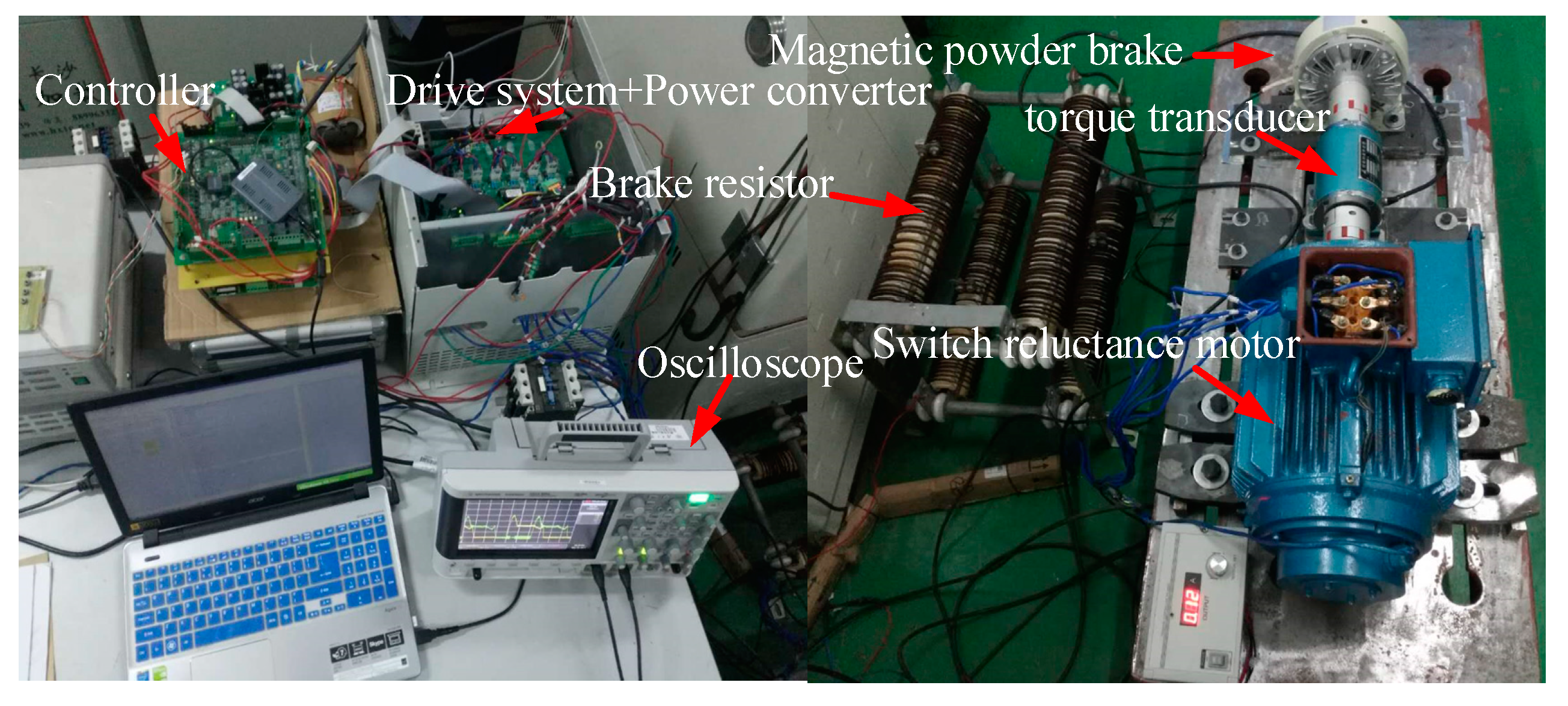
A three-phase 12/8 SRM experimental system was built, and an asymmetric half-bridge converter was employed in Figure 19. Specification of SRM and the equipment are shown in

Table 5. Specification of switched reluctance motor (SRM).

Number of Stator/Rotor Poles	12/8
Rated speed	1190 rev/min
Rated voltage	200 V
Phase resistance	0.1 ohm

and

Table 6. List of equipment.

DSP	TMS320F28335
Torque transducer	JN338
Magnetic power brake	FZ-J
Adjustable DC power supply (for power brake)	KD-200A
Converter	Asymmetric half-bridge
Current sensor	ETCR035AD
Rotary transformer	TS2660N141E64

respectively. Phase current was acquired by using a high-precision ETCR035AD current sensor (ETCR, Guangzhou, China), the reference rotor position was obtained by using the Tamagawa TS2660N141E64 rotary transformer (Tamagawa, Iida, Japan), and AU6802E chip (Tamagawa, Iida, Japan) was used to decode the cosine signal of the position chip.

The motor rotating through a 360° mechanical angle corresponded to 16,348 points. The frequency of the chopping current and injected voltage pulses were set to 10 kHz, and the voltage duty cycle was selected as 30% to improve the inductor calculation accuracy. The angles 180° and 360° represent the unaligned and aligned position of the motor (electrical angle). In addition, turn-on and turn-off angles were set to 182° and 355°, respectively (electrical angle).

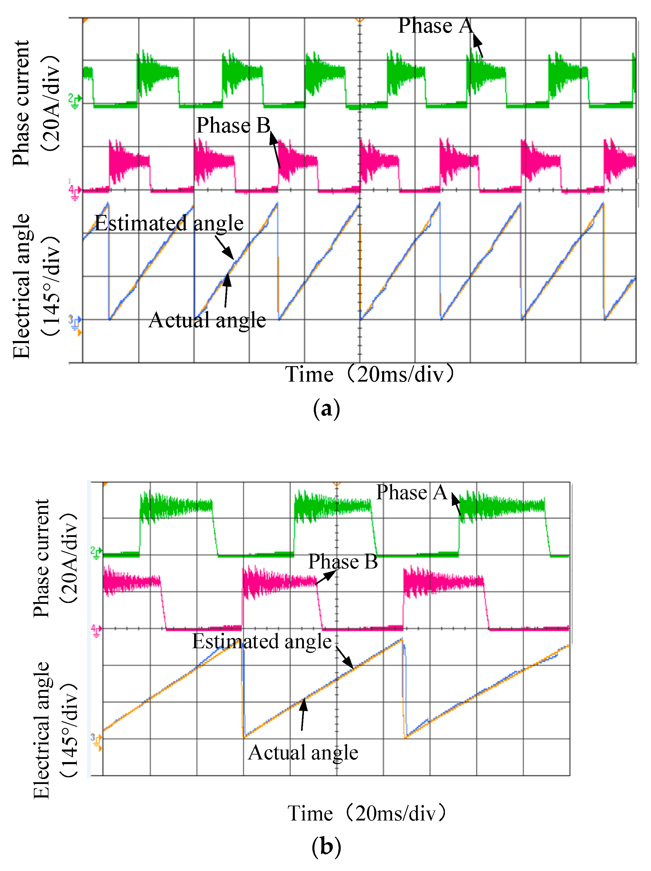
All experimental loadings were performed by using a magnetic powder brake, thereby resulting in the inevitable fluctuation of motor speed within a certain range. First, the motor was operated at light load with the reference current defined as 15 A. The waveforms of the phase current, actual position, and estimated position are shown in Figure 20a. It can be viewed that the estimated position matched the actual angle well by using the proposed method and the position error was within 0.5° (mechanical angle). The given motor phase current was set to 22 A, motor operation under magnetic saturation was ensured, and the waveforms of voltage and current and actual position are shown in Figure 20b. The error of the estimated position angle and the actual angle was within 0.9° (mechanical angle).

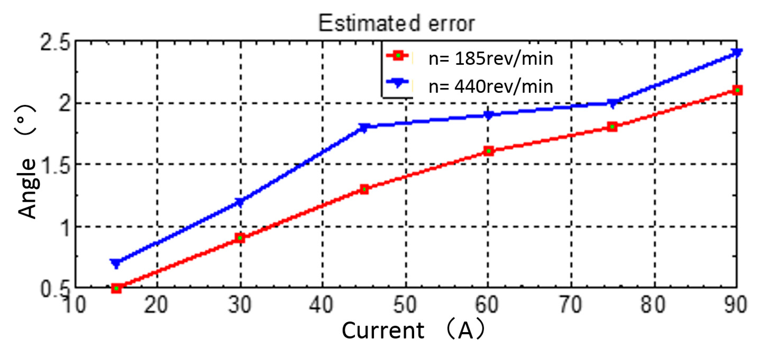
The error between the estimated position and the measurement is present in Figure 21, where the error did not significantly increase as the speed increased. However, when the speed exceeded the rated speed, the error significantly increased due to the delay between the sampling instant and the calculated instant. Results of the experimental (Figure 21) and the simulation results (Figure 18) matched well, and high accuracy of the position was obtained with the application of the proposed sensorless control scheme.

6. Conclusions

In this paper, a generalized position sensorless control strategy considering the magnetic saturation for an SRM drive system is proposed. The position was estimated based on six special inductance intersection positions. The simulation and experiment verified the effectiveness of the method. The findings are as follows. First, six inductance intersections were available per 360° electrical angle, where speed and position estimation can be updated six times, and the accuracy of speed and position estimation in operation can be guaranteed. Furthermore, the inductance characteristics were fully utilized to estimate the rotor position. The intersection position in the low-inductance area, which was slightly affected by magnetic saturation, could directly serve as an update point. Moreover, the intersection position in the high-inductance region could be calculated by using a prior polynomial fitting function and the sampling phase current.

Finally, obtaining the mapping relationship between the inductance and the position angles of this method in advance was unnecessary. Compared with the traditional technique, the number of available update points for speed and position estimation was increased to 48. Consequently, the adaptability was increased even when the motor was operated at low speed or at an unstable speed. In addition, the accuracy of position estimation for the heavy load condition was improved.