Experimental and Theoretical Research on Bending Behavior of Photovoltaic Panels with a Special Boundary Condition

Abstract

Currently, the photovoltaic (PV) panels widely manufactured on market are composed of stiff front and back layers and the solar cells embedded in a soft polymeric interlayer. The wind and snow pressure are the usual loads to which working PV panels need to face, and it needs the panels keep undamaged under those pressure when they generate electricity. Therefore, an accurate and systematic research on bending behavior of PV panels is important and necessary. In this paper, classical lamination theory (CLT) considering soft interlayer is applied to build governing equations of the solar panel. A Rayleigh–Rita method is modified to solve the governing equations and calculate the static deformation of the PV panel. Different from many previous researches only analyzing simply supported boundary condition for four edges, a special boundary condition which consists of two opposite edges simply supported and the others two free is studied in this paper. A closed form solution is derived out and used to do the numerical calculation. The corresponding bending experiments of PV panels are completed. Comparing the numerical results with experiment results, the accuracy of the analytical solutions are verified.

1. Introduction

According to the report from Ministry of Housing and Urban–Rural Department of China, building consumes 40% to 50% of the total energy in China each year, which is one of the main reasons for the aggravation of energy consumption. Solar energy is a green and renewable energy, and it is widely spread around the world. Several technologies have been developed to use solar energy generating electricity. If solar energy can be used in the building, it will cut down the external energy consumed by the building and the total energy consumption will be reduced significantly. Among the existed technologies applying solar energy in buildings, building integrated photovoltaic (BIPV) has gained a great of attention and great advances in recent years. The main difference between building attached photovoltaic (BAPV) and BIPV is that the photovoltaic (PV) module is designed and constructed with buildings at the same time in BIPV, which makes it as one part of the building structure. When the BIPV building is running, on one hand, the PV components can generate electricity to realize the energy reduction. On the other hand, the PV components need to bear the external loads and behave as structural parts to ensure the safety of building.

The research and application of BAPV started from 1970s, while BIPV became commercially available two decades later [1]. In 2014, U.S. National Renewable Energy Laboratory (NREL) promulgated an economic assessment and brief overview, in which the history of BIPV was summarized and some challenges about the BIPV future were stated [2]. Meanwhile, the zero emission energy building European target for 2020 [3] was presented and the research works about BIPV became more meaningful. In several review papers [4,5,6,7], the history, development and future opportunities of BIPV are stated carefully and it denotes that the needs of BIPV in next several decades are still huge. However, it shows that the mechanical behavior of the BIPV products are studied much less than energy efficiency and temperature change. Peng etc. [8] pointed out that the building loads and PV module damage situation should be considered seriously in BIPV too.

Currently, there are several different types of PV modules existed in the market. All of them choose glass as the cover plate to make sure the absorption and transmission of sunlight. As to the bottom plate, it can be made of the transparent glass or opaque TPT, which makes double glass PV module or single glass PV module. Due to the requirements of lighting inside the building, the double glass PV module with better photopermeability are more suitable and acceptable in the real structures. Therefore, the PV panels studied in the present paper focusing on BIPV are double glass PV module which consists of two glasses and an interlayer in where the cells are sealed by ethylene vinyl acetate (EVA) or polyvinyl butyral (PVB).

When the double glass PV module is adopted in the building as BIPV, it needs to bear external loads to keep the structure safe. Especially, the snow load to roof and wind load to the window must be analyzed carefully. However, there is not any specific certification to provide the requirements on the double glass PV panel for bearing those loads. Only in the standard of PV module itself, IEC 61215 (2005) [9], the bending test under 2.4 KPa uniformly distributed force is required to all commercial PV module. It is still unknown if that test standard can ensure the safety of double glass PV module worked as building components, so further researches must be made in here to understand their bending behavior clearly and develop some relative requirements.

Among the few studies about bending behavior of PV panel, Naumenko and Eremeyev [10] believed that PV panel is a layered composite with relatively stiff skin layer and relatively soft core, since the ratio of shear moduli $\mu =G_C/G_S$ for core material to skin glass is in the range between 10⁻⁵ and 10⁻². They derived the differential equations for primary unknowns based on layer-wise theory, but the equations were only solved for plate strip with simply supported boundary condition. Eisentrager etc. [11] applied layer-wise theory to analyze the bending behavior of PV module and laminated glass panel, and they presented a finite element formulation and a user-defined quadrilateral serendipity element. Eisentrager etc. [12] also adopted first order shear deformation theories (FSDT) to study the PV panel and laminated glass with weak shear stiffness. A user-defined element is still developed and integrated with ABAQUS. In real buildings, some of the roofs or walls need to be designed as unsymmetrical laminates in order to make lightweight construction, so Weps [13] choose them to do the research. A three-point bending test is performed and used to verify the proposed equations and finite element analysis. Similar works on symmetrical laminated glass beam for PV application are completed by Schulze etc. [14].

As to the theories and mechanic models for laminate composite, Vedrtnam and Pawar [15] made a review work on them and their introductions are mainly about the laminate glass plate which is extremely similar to PV panel. First order shear deformation theory (FSDT) is a widely-used approach for laminate composite, and the analytical solution or semi-analytical solution based on it are proposed and verified in many works [16,17,18,19,20,21,22]. Zig-zag theory applies the piecewise functions to represent displacements of the plate with respect to the thickness coordinate, and the governing equations can be simplified a lot [23,24,25,26]. Layer-wise theory (LWT) is chosen by many researchers to study PV module. In LWT, the constitutive equations are derived for each layer itself, and interaction forces and compatibility are described more precisely [10,11,13,27,28,29,30,31,32]. Except those, researchers also proposed some other theories and models, such as trigonometric shear deformation theory [33], new higher order shear deformation theory [34,35], and so on. Then, the methods to solve the different partial differential equations are also developed by many researchers [36,37,38]. However, in many of those works, the boundary conditions of the plates are only simply-supported for four edges since it is easier to solve the equations and get solutions.

In present paper, the bending behavior of double glass PV panel is studied carefully by both experimental and theoretical research. Different from many previous researches, a special boundary condition which is two opposite edges free and the other two edges simply-supported (annotated as SSFF) is considered. Although LWT has been used previously in PV module research, Hoff model which is one of the classical lamination theory (CLT) is adopted in this research. By developing a modified Rayleigh–Rita method, a closed-form solution is derived out. The experiment is designed using water pressure to produce uniformly distributed force, so it is much more accurate than other research works using sand or brick. A frame is manufactured to simulate the special boundary condition. Comparing the theoretical results with experimental results, the accuracy of the analytical solutions are verified. The theoretical model and solutions obtained in present work will be the fundamentals for the optimal design work in future.

2. Theoretical Analysis of Double Glass PV Panel

As studied by Naumenko and Eremeyev [10], the main feature of double glass PV panel is the thin and relatively low shear moduli of interlayer comparing with the glass layer. A proper mechanical model is very important to describe the force transfer and deformation of the panel. Hoff model is one of the classical lamination theory, and it can analyze the laminate composite with soft core precisely. Therefore, Hoff model is applied to simulate PV panel and the corresponding governing equations are derived. Then, due to the special boundary condition, Rayleigh–Rita method is modified and utilized to obtain the closed-form solution for the bending deflection of PV panel with SSFF. At last, the strain and stress of each layer are calculated by the bending deflection.

2.1. Mechanical Model and Basic Hypothesis

The basic components of double glass PV panel are shown in Figure 1, including cover glass, ethylene-vinylacetate (EVA), silicon solar cells, and back glass. Since silicon solar cells are so thin and fragile, they are embedded in the EVA material to be protected. According to the results from Naumenko and Eremeyev [10], the EVA material layer carries out almost all the shear stress of interlayer while the bending moment and normal force are very small and can be negligible. In order to simplify the problem and emphasize the main characters of the PV panel, a laminate plate model is applied and several hypothesizes are made at the beginning of the structural analysis as follows.

(1)

The cover and backboard glasses are treated as top and bottom surfaces of the laminate plate, respectively. And both of them are simulated as isotropic plates with constant flexural rigidity.

(2)

The silicon solar cells are too thin to bear any shear stress, and two EVA layers play the main role of interlayer. The silicon solar cell layer is ignored and two EVA layers are merged as one layer which is defined as the interlayer only made of EVA. The whole PV panel is simplified as a three-layer composite, including cover plate, interlayer and back plate. The mechanical model of PV panel under uniformly distributed force and the corresponding coordinate system are shown in Figure 2.

(3)

According to the research results summarized by Naumenko and Eremeyev [10] and Stefan-H. Schulze etc. [14], in PV module, the ratio of the shear moduli between interlayer and surface layer is in the range between 10⁻⁵ and 10⁻². The PV module is a typical soft core laminate plate and the stress of the interlayer in x-y plan should be ignored.

(4)

Only the anti-symmetrical deformation is studied in present paper, so the stress ${\sigma }_z$ and the strain ${\epsilon }_z$ of interlayer are very small and can be ignored, which is defined as ${\sigma }_z= 0$, ${\epsilon }_z= 0$.

2.2. Hoff Model and Governing Equations

Hoff [39] modified Reissner theory and developed a Hoff model for laminated plate. In Hoff model, the flexural rigidities of surface plates are calculated but the interlayer is a relative soft layer. As introduced in Section 2.1, PV panels are just a kind of laminate plate structure with soft core and Hoff model (as shown in Figure 2) is very suitable to represent them. According to Hoff model and based on those hypothesizes, the governing equations of the PV panels can be derived as

$$D\left(\frac{{\partial }^2{\phi }_x}{\partial x^2}+\frac{1-{\nu }_f}{2}\frac{{\partial }^2{\phi }_x}{\partial y^2}+\frac{1+{\nu }_f}{2}\frac{{\partial }^2{\phi }_y}{\partial x\partial y}\right)+C\left(\frac{\partial w}{\partial x}-{\phi }_x\right)=0$$

(1)

$$D\left(\frac{{\partial }^2{\phi }_x}{\partial x^2}+\frac{1-{\nu }_f}{2}\frac{{\partial }^2{\phi }_x}{\partial y^2}+\frac{1+{\nu }_f}{2}\frac{{\partial }^2{\phi }_y}{\partial x\partial y}\right)+C\left(\frac{\partial w}{\partial x}-{\phi }_x\right)=0$$

(2)

$$C\left({\nabla }^{2}w-\frac{\partial {\phi }_x}{\partial x}-\frac{\partial {\phi }_y}{\partial y}\right)-2D_f{\nabla }^2{\nabla }^{2}w+q=0$$

(3)

where ${\phi }_x$, ${\phi }_y$ and $w$ are unknown variables as cross section rotation at x-z plane, y-z plane and deflection at z direction, respectively. Constant variables D, $D_f$ and C are defined as Equations (9)–(11). In order to simplify the governing equations, two functions $\omega$ and $f$ are introduced and they are defined as Equations (4) and (5).

$${\phi }_x=\frac{\partial \omega }{\partial x}+\frac{\partial f}{\partial y}$$

(4)

$${\phi }_y=\frac{\partial \omega }{\partial y}-\frac{\partial f}{\partial x}$$

(5)

With Equations (1)–(3) and Equations (4) and (5), we could obtain the modified governing equations of PV panel under uniformly distributed force as

$$w=\omega -\frac{D}{C}{\nabla }^2\omega$$

(6)

$$\left(D+2D_f\right){\nabla }^2{\nabla }^2\omega -\frac{2D{D}_f}{C}{\nabla }^2{\nabla }^2{\nabla }^2\omega =q$$

(7)

$$\frac{1}{2}D\left(1-{\nu }_f\right){\nabla }^{2}f-Cf=0$$

(8)

with

$$D=\frac{E_f{\left(h+t\right)}^{2}t}{2\left(1-{\nu }_f{}^2\right)}$$

(9)

$$D_f=\frac{E_f{t}^3}{12\left(1-{\nu }_f{}^2\right)}$$

(10)

$$C=G_C\frac{{\left(h+t\right)}^2}{h}$$

(11)

where $E_f$ is the elastic modulus of the cover and the back glass plate, $v_f$ is the Poisson’s ratio of the cover and the back glass plate, $G_C$ is the shear modulus of EVA, t and h are the thickness of surface plate and EVA interlayer, respectively.

2.3. Special Boundary Condition

In previous researches, in order to simplify the problem, all four edges with simply supported boundary condition (as shown in Figure S1) is mostly studied. However, it is different in some accessory structures, such as glass eave or glass shutter. In those structures, the glasses or PV panels adopt the boundary condition SSFF and the analysis of it is limited. In present paper, that special boundary condition is studied carefully and the closed-form solution of it is derived out. As shown in Figure S2, the PV panel is simply supported at the edges x = 0 and a, and free–free at the edges $y=\pm 0.5b$.

The boundary condition studied in present paper should satisfy the formulas as follows.

$${\left(M_x^{\prime }\right)}_{x=0,a}=0, {\left(w\right)}_{x=0,a}=0, {\left({\phi }_y\right)}_{x=0,a}=0, {\left(M_x^{″}\right)}_{x=0,a}=0$$

(12)

$$\left(M_y^{\prime }\right){}_{y =\pm \frac{b}{2}}=0, \left(M_{xy}^{\prime }\right){}_{y =\pm \frac{b}{2}}=0, \left(M_{xy}^{″}\right){}_{y =\pm \frac{b}{2}}=0, \left(Q_y\right){}_{y =\pm \frac{b}{2}}=0, {\left(M_y^{″}\right)}_{y=\pm \frac{b}{2}}=0$$

(13)

At the edges x = 0 and a, Equation (12) can be derived out as follows.

$$\frac{\partial {\phi }_x}{\partial x}=0,{\phi }_y=0,w=0,\frac{{\partial }^{2}w}{\partial x^2}=0$$

(14)

Combining with Equations (4) and (5) and following the procedure derived by previous research work, we can obtain Equation (15) based on Equation (12).

$$\omega ={\nabla }^2\omega ={\nabla }^4\omega =0,\frac{\partial f}{\partial x}=0$$

(15)

At the edges $y=\pm 0.5b$, the boundary condition is very different from those studied before and so a specific derivation is stated. According to the stress–strain relationship of laminated plate [39], the Equation (13) could be rewritten as follows.

$$-D\left(\frac{\partial {\phi }_y}{\partial y}+{\nu }_f\frac{\partial {\phi }_x}{\partial x}\right)=0$$

(16)

$$-2D_f\left(\frac{{\partial }^{2}w}{\partial y^2}+{\nu }_f\frac{{\partial }^{2}w}{\partial x^2}\right)=0$$

(17)

$$-\frac{1}{2}\left(1-{\nu }_f\right)D_f\left(\frac{\partial {\phi }_x}{\partial y}+\frac{\partial {\phi }_y}{\partial x}\right)=0$$

(18)

$$-2\left(1-{\nu }_f\right)D_f\frac{{\partial }^{2}w}{\partial x\partial y}=0$$

(19)

$$C\left(\frac{\partial w}{\partial y}-{\phi }_y\right)-2D_f\left(\frac{{\partial }^{3}w}{\partial x^2\partial y}+\frac{{\partial }^{3}w}{\partial y^3}\right)=0$$

(20)

Equations (16) and (5) can yield

$$\frac{{\partial }^2\omega }{\partial y^2}-\frac{{\partial }^{2}f}{\partial x\partial y}+{\nu }_f\frac{{\partial }^2\omega }{\partial x^2}+{\nu }_f\frac{{\partial }^{2}f}{\partial x\partial y}=0$$

(21)

Equations (17) and (6) can yield

$$\frac{{\partial }^2\omega }{\partial y^2}-\frac{D}{C}\left(\frac{{\partial }^4\omega }{\partial x^2\partial y^2}+\frac{{\partial }^4\omega }{\partial y^4}\right)+{\nu }_f\frac{{\partial }^2\omega }{\partial x^2}--\frac{D}{C}{\nu }_f\left(\frac{{\partial }^4\omega }{\partial x^4}+\frac{{\partial }^4\omega }{\partial x^2\partial y^2}\right)=0$$

(22)

Equations (19) and (6) can yield

$$\frac{{\partial }^2\omega }{\partial x\partial y}-\frac{D}{C}\left(\frac{{\partial }^4\omega }{\partial x^3\partial y}+\frac{{\partial }^4\omega }{\partial x\partial y^3}\right)=0$$

(23)

At last, Equations (20) and (6) could yield

$$-D\left(\frac{{\partial }^3\omega }{\partial x^2\partial y}+\frac{{\partial }^3\omega }{\partial y^3}\right)+C\frac{\partial f}{\partial x}-2D_f\left[\frac{{\partial }^3\omega }{\partial x^2\partial y}+\frac{{\partial }^3\omega }{\partial y^3}-\frac{D}{C}\left(\frac{{\partial }^5\omega }{\partial x^4\partial y}+2\frac{{\partial }^5\omega }{\partial x^2\partial y^3}+\frac{{\partial }^5\omega }{\partial y^5}\right)\right]=0$$

(24)

Equations (14) and (21)–(24) are the specific formulas for the special boundary condition discussed in present paper, and they will be applied in the derivation work for closed-form solution of deflection.

2.4. Modified Rayleigh–Rita Method and Closed-Form Solutions

Rayleigh–Rita method is a useful way to solve the partial differential equations, and it uses the expansion of the unknown functions of deflection in infinite series form. It is possible to approach or be close to the exact solutions of the equations by taking the sufficient number of the terms in the series. A modified Rayleigh–Rita method is applied in present paper due to the special boundary condition, and the closed-form solutions of the governing equations could be obtained. Since the boundary condition is simply supported at edges x = 0 and a, the sinusoidal function should be utilized and the unknown variable ω and f is assumed as

$$\omega ={\displaystyle \sum _{n=1}^{\infty }\left(e^{{\lambda }_{n}y}{\omega }_n+{\omega }^{*}\right)\sin \left(k_{n}x\right)}$$

(25)

$$f={\displaystyle \sum _{n=1}^{\infty }{e}^{{\eta }_{n}y}{f}_n\cos \left(k_{n}x\right)}$$

(26)

where $k_n=n\pi /a$; ${\displaystyle \sum _{n=1}^{\infty }\left(e^{{\lambda }_{n}y}{\omega }_n\right)\sin \left(k_{n}x\right)}$ and ${\displaystyle \sum _{n=1}^{\infty }{e}^{{\eta }_{n}y}{f}_n\cos \left(k_{n}x\right)}$ are the general solutions; ${\displaystyle \sum _{n=1}^{\infty }\left({\omega }^{*}\right)\sin \left(k_{n}x\right)}$ is the specific solution; ${\lambda }_n$, ${\omega }_n$, ${\omega }^{*}$, ${\eta }_n$ and $f_n$ are unknown variables needed to be solved.

The general solution of Equation (7) is studied firstly, so the assumption of general solution, $\omega ={\displaystyle \sum _{n=1}^{\infty }\left(e^{{\lambda }_{n}y}{\omega }_n\right)\sin \left(k_{n}x\right)}$, is substituted into Equation (27).

$$\left(D+2D_f\right){\nabla }^2{\nabla }^2\omega -\frac{2D{D}_f}{C}{\nabla }^2{\nabla }^2{\nabla }^2\omega =0$$

(27)

By merging the same terms, the characteristic equation is written as

$$A_2{\lambda }_n^6-\left(A_1+3A_2{k}_n^2\right){\lambda }_n^4+\left(2A_1{k}_n^2+3A_2{k}_n^4\right){\lambda }_n^2-\left(A_1{k}_n^4+A_2{k}_n^6\right)=0$$

(28)

with

$$A_1=D+2D_f$$

(29)

$$A_2=\frac{2D{D}_f}{C}$$

(30)

Defining $\overline{a}=A_2$, $\overline{b}=-\left(A_1+3A_2{k}_n^2\right)$, $\overline{c}=\left(2A_1{k}_n^2+3A_2{k}_n^4\right)$, $\overline{d}=-\left(A_1{k}_n^4+A_2{k}_n^6\right)$, Equation (28) is also rewritten as Equation (31).

$$\overline{a}{\lambda }_n^6+\overline{b}{\lambda }_n^4+\overline{c}{\lambda }_n^2+\overline{d}=0$$

(31)

Equation (31) is a sextic equation and there are not extract root formulas for it. However, it could be solved as following. By defining a new variable, $S={\lambda }^2+\frac{\overline{b}}{3\overline{a}}$, Equation (31) is transformed as

$$S^3+PS+R=0$$

(32)

with

$$P=\frac{1}{\overline{a}}\left(\overline{c}-\frac{{\overline{b}}^2}{3\overline{a}}\right)$$

(33)

$$R=\frac{1}{\overline{a}}\left(\overline{d}+\frac{2{\overline{b}}^3}{27{\overline{a}}^2}-\frac{\overline{b}\overline{c}}{3\overline{a}}\right)$$

(34)

The roots of the cubic Equation (32) can be solved by

$$S_1={\Delta }_1+{\Delta }_2,S_2=\overline{\omega }{\Delta }_1+{\overline{\omega }}^2{\Delta }_2,S_1={\overline{\omega }}^2{\Delta }_1+\overline{\omega }{\Delta }_2$$

(35)

where ${\Delta }_1=\sqrt[3]{-\frac{R}{2}+\sqrt{{\left(\frac{R}{2}\right)}^2+{\left(\frac{P}{2}\right)}^3}}$, ${\Delta }_2=\sqrt[3]{-\frac{R}{2}-\sqrt{{\left(\frac{R}{2}\right)}^2+{\left(\frac{P}{2}\right)}^3}}$ and $\overline{\omega }=\frac{-1+i\sqrt{3}}{2}$.

According to the defination of S, the roots of Equation (28) are finally sovled as ${\lambda }_{n1},{\lambda }_{n2}=\pm i{\beta }_1$, ${\lambda }_{n3},{\lambda }_{n4}=\pm i{\beta }_2$ and ${\lambda }_{n5},{\lambda }_{n6}=\pm i{\beta }_3$, in where the varaibles β could be calculated by

$${\beta }_j=\sqrt{\frac{\overline{b}}{3\overline{a}}-S_j},j=1,2,3$$

(36)

The six roots of the characteristic Equation (28) has been solved and the general solution of Equation (7) should be written in the format as Equation (37).

$$\overline{\omega }={\displaystyle \sum _{n=1}^{\infty }\left[{\displaystyle \sum _{r=1}^6{e}^{{\lambda }_{nr}y}{\omega }_{nr}}\right]\sin \left(k_{n}x\right)}$$

(37)

Then, the specific solution of Equation (7) shoulde be solved to satisfy Equation (38).

$$\left(D+2D_f\right){\nabla }^2{\nabla }^2{\overline{\omega }}^{*}-\frac{2D{D}_f}{C}{\nabla }^2{\nabla }^2{\nabla }^2{\overline{\omega }}^{*}=q$$

(38)

Bending behavior of PV panel under uniformlly distributted force is studied in present paper, so the force q is a constant. Taking the Fourier expansion and doing odd continuation on the right term in Equation (38), it can be expressed as

$$q=\frac{2}{a}{\displaystyle \sum _{n=1}^{\infty }\left[{\displaystyle {\int }_0^{a}q\sin \frac{n\pi x}{a}dx}\right]\sin \frac{n\pi x}{a}}={\displaystyle \sum _{n=1}^{\infty }\left\{\frac{2q}{n\pi }\left[1-\cos \left(n\pi \right)\right]\right\}\sin \frac{n\pi x}{a}}$$

(39)

Substituting Equation (39) into Equation (38), the specific solution can be solved as follows.

$${\overline{\omega }}^{*}={\displaystyle \sum _{n=1}^{\infty }\left\{\frac{2q}{n\pi }\left[1-\cos \left(n\pi \right)\right]\frac{1}{A_1{k}_n^4+A_2{k}_n^6}\right\}\sin \left(k_{n}x\right)}$$

(40)

The full solution of Equation (7) consists of the general solution and specific solution, and it could be denoted specifically as

$$\omega ={\displaystyle \sum _{n=1}^{\infty }\left\{\left[{\displaystyle \sum _{r=1}^6{e}^{{\lambda }_{nr}y}{\omega }_{nr}}\right]+\frac{2q}{n\pi }\left[1-\cos \left(n\pi \right)\right]\frac{1}{A_1{k}_n^4+A_2{k}_n^6}\right\}\sin \left(k_{n}x\right)}$$

(41)

The same procedure could be applied to solve Equation (8) with the solution assumption as shown in Equaiton (26), so the solution of Equation (8) could be denoted by

$$f={\displaystyle \sum _{n=1}^{\infty }\left({\displaystyle \sum _{r=1}^2{e}^{{\eta }_{nr}y}{f}_{nr}}\right)\cos \left(k_{n}x\right)}$$

(42)

where

$$A_3=\frac{1}{2}D\left(1-{\nu }_f\right)$$

(43)

$${\eta }_{n1}=\sqrt{\frac{C}{A_3}+k_n^2}$$

(44)

$${\eta }_{n2}=-\sqrt{\frac{C}{A_3}+k_n^2}$$

(45)

The full solutions of Equations (7) and (8) could be calculated by Equations (41) and (42), respectively. However, there are total eight unkown variables in the solutions, including ${\omega }_{nr}$ (r = 1 to 6) and $f_{nr}$ (r = 1 and 2). The boudnary conditions stated as Equations (21)–(24) are applied in here to obtain the exact values of those unknown variables. Substituting Equations (41) and (42) into Equations (21)–(24), the eight unknown variables must satisfy the following equations.

$${\displaystyle \sum _{r=1}^6\left[{\lambda }_{nr}^2{e}^{{\lambda }_{nr}y}+v_f\left(-k_n^2\right)e^{{\lambda }_{nr}y}\right]}{\omega }_{nr}+{\displaystyle \sum _{r=1}^2\left[v_f{\eta }_{nr}\left(-k_n\right)e^{{\eta }_{nr}y}-{\eta }_{nr}\left(-k_n\right)e^{{\eta }_{nr}y}\right]}{f}_{nr}=v_f{\overline{\omega }}^{*}{k}_n^2$$

(46)

$${\displaystyle \sum _{r=1}^6\left[\begin{array}{l}{\lambda }_{nr}^2-\frac{D}{C}{\lambda }_{nr}^2\left(-k_n^2\right)-\frac{D}{C}{\lambda }_{nr}^4\\ +v_f\left(-k_n^2\right)-v_f\frac{D}{C}{k}_n^4-v_f\frac{D}{C}{\lambda }_{nr}^2\left(-k_n^2\right)\end{array}\right]}{e}^{{\lambda }_{nr}y}{\omega }_{nr}=v_f{\overline{\omega }}^{*}{k}_n^2+v_f\frac{D}{C}{\overline{\omega }}^{*}{k}_n^4$$

(47)

$${\displaystyle \sum _{r=1}^6\left[k_n{\lambda }_{nr}+\frac{D}{C}{k}_n^3{\lambda }_{nr}-\frac{D}{C}{k}_n{\lambda }_{nr}^3\right]}{e}^{{\lambda }_{nr}y}{\omega }_{nr}=0$$

(48)

$${\displaystyle \sum _{r=1}^6\left[\begin{array}{l}D{\lambda }_{nr}{k}_n^2-D{\lambda }_{nr}^3+2D_f{\lambda }_{nr}{k}_n^2-2D_f{\lambda }_{nr}^3\\ +\frac{2D_{f}D}{C}{\lambda }_{nr}{k}_n^4+\frac{4D_{f}D}{C}{\lambda }_{nr}^3\left(-k_n^2\right)+\frac{2D_{f}D}{C}{\lambda }_{nr}^5\end{array}\right]}{e}^{{\lambda }_{nr}y}{\omega }_{nr}+{\displaystyle \sum _{r=1}^{2}C\left(-k_n\right)e^{{\eta }_{nr}y}{f}_{nr}}=0$$

(49)

Substituting $\mathrm{y}=\pm 0.5b$, there are eight equations for eight unknown variables based on Equations (46)–(49), and all variables could be solved to get exact values. Once ω is solved by Equation (41), the deflection of PV panel under uniformly distributed force could be calculated based on Equation (6) as

$$\begin{array}{l}w=\omega -\frac{D}{C}{\nabla }^2\omega ={\displaystyle \sum _{n=1}^{\infty }\left\{{\displaystyle \sum _{r=1}^6{e}^{{\lambda }_{nr}y}{\omega }_{nr}}+\frac{2q}{n\pi }\left[1-\cos \left(n\pi \right)\right]\frac{1}{A_1{k}_n^4+A_2{k}_n^6}\right\}\sin \left({\mathrm{k}}_{n}x\right)}\\ -\frac{D}{C}{\displaystyle \sum _{n=1}^{\infty }\left\{{\displaystyle \sum _{r=1}^6\left[\left(-k_n^2\right)e^{{\lambda }_{nr}y}{\omega }_{nr}+{\lambda }_{nr}^2{e}^{{\lambda }_{nr}y}{\omega }_{nr}\right]}+\left(-k_n^2\right)\frac{2q}{n\pi }\left[1-\cos \left(n\pi \right)\right]\frac{1}{A_1{k}_n^4+A_2{k}_n^6}\right\}\sin \left({\mathrm{k}}_{n}x\right)}\end{array}$$

(50)

2.5. Finite Element Analysis

To verify the results of Hoff model used above, a finite element analysis is performed by the use of FEM software ANSYS. The double glass PV panels are simplified as a five layers composite structure, and the material of each layer is simulated as isotropic material. The mechanical properties of the model materials are shown in

Table 1. Material parameter values.

Material	Parameter Values
	Modulus of Elasticity/MPa	Poisson Ratio	Thickness/mm
Reinforced glass	7.2 × 104	0.2	2
Crystalline silicon battery	1.44 × 105	0.28	0.2
EVA	3.5 × 10	0.3	0.8

. Considering the element characteristics that it could be layered, four-node SHELL181 composite shell element is used for modeling (as shown in Figure S3). The rectangular shell structure is divided into five layers which are cover glass, EVA, silicon battery sheet, EVA and back glass, respectively. Since it’s too thin to make any influence, the battery layer is assumed as a continuous layer.

Besides three displacement degrees of freedom (DOF), the SHELL element has extra three rotation DOFs at each node, comparing with the SOLID element. In order to simulate the boundary conditions accurately, two long edges parallel to the Y axis are fixed in the Z direction while the other two short edges parallel to the X axis are completely free. The node constraints of both X and Y directions are applied at the four corners (as shown in Figure S3). By doing in this way, it can simulate the special boundary condition studied in present paper.

3. Experimental Analysis of Double Glass PV Panel

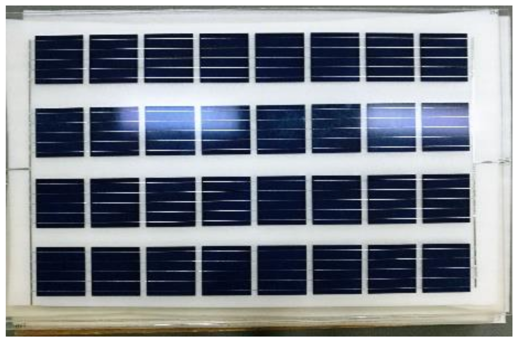
In order to verify the structural analysis results and test the real mechanical properties of PV panels, bending testing is performed for 8 specimens at room temperature. The specimens are all the double glass photovoltaic modules (as shown in Figure 3) which are provided by Suzhou Tenghui Photovoltaic Technology Co., Ltd (Changshu, China). Among those specimens, there are 3 specimens with size 1658 × 995 × 5 (unit: mm) and 3 specimens with size 1658 × 995 × 7.4 (unit: mm). The two groups of PV panels are different at the thickness of the glass. The cover and back glasses are 2 mm for first group and 3.2 mm for the second group, but the thickness of interlayer is same as 1 mm.

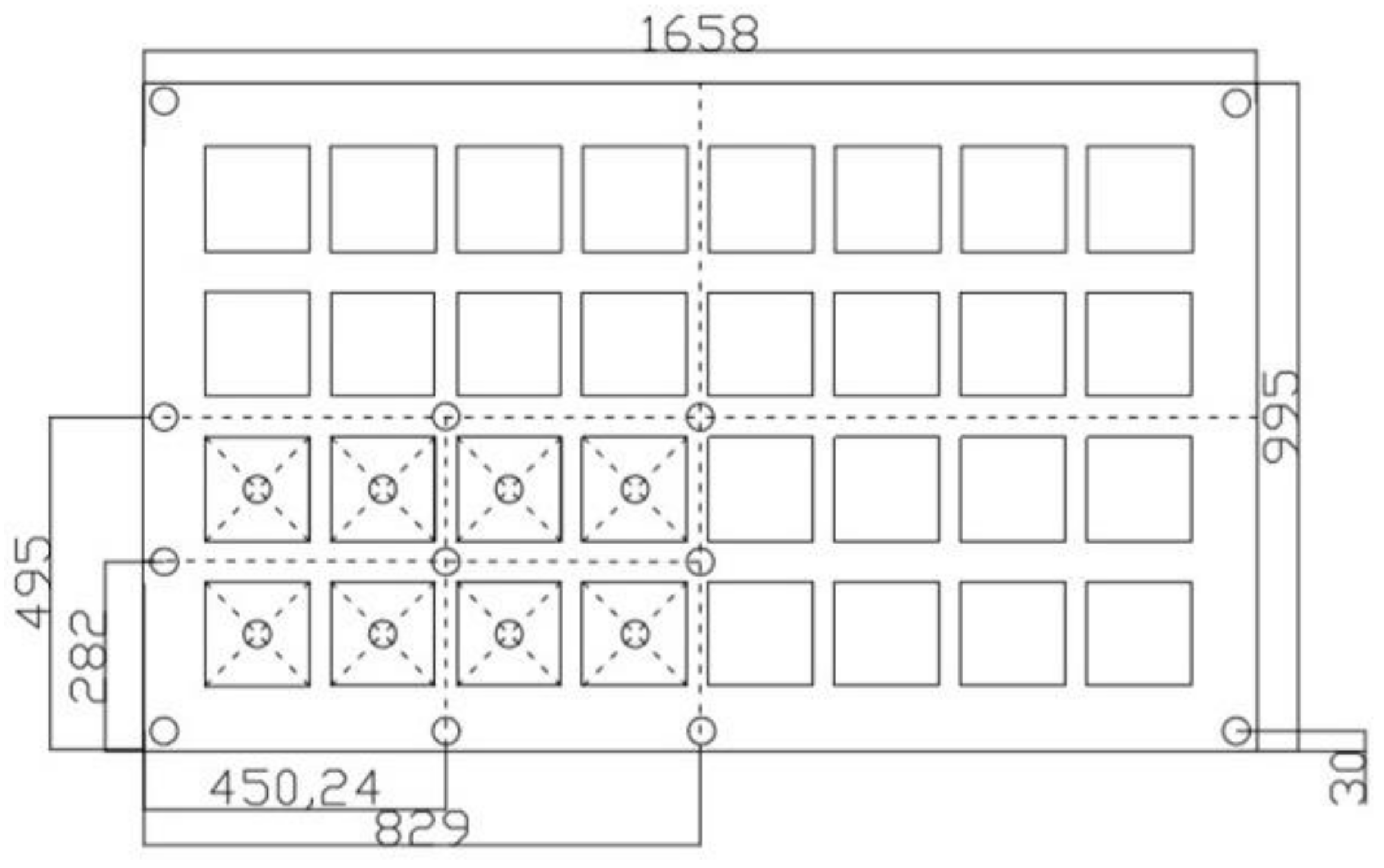
The bending test was completed in National Photovoltaic Product Quality Supervision and Inspection Center at Chengdu, referring to the current quality inspection certification, IEC 61215 [9]. The test frame (as shown in Figure 4) can simulate the discussed special boundary condition SSFF. Due to the symmetry of PV panel and the loading, the strain measurement points are only set on a quarter part of the panel with total 20 points, which is shown as Figure 5. The PV panel strains are collected by DH3816 static strain gauge, and the deflection at panel center is measured by a laser displacement meter installed under the panel. In previous experimental works, sands or bricks were usually used to make uniformly distributed force but they are not so accurate. Different from those works and due to its better fluidity, water pressure is applied in present paper to simulate the uniformly distributed force. The loading plan is different for two groups of PV panels since the bending behavior of them are different. As to the 5 specimens with 2 mm glass, it adds 0.5 kPa at each level until maximum pressure 2.5 kPa, then it unloads 0.5 kPa at each step until back to 0 kPa (as shown in Figure S4). In the experiments of 3 specimens with 3.2 mm glass, the water pressure is added 1 kPa at each step until reaching maximum pressure 4 kPa, and it is unloaded 1 kPa for each level until 0 kPa pressure (as shown in Figure S4). The duration time of the load per stage is same as 8 min, so the deformation of bending panel can be measured precisely. Water proof cloth, which is installed on the PV panel as Figure 6, is used to protect the strain gauge from water and it can help making water pressure applied evenly on the whole PV panel.

4. Verifications and Discussions

4.1. Experiment Results

The bending test was completed at an indoor temperature, 25 °C. The central deflections of the specimens with 2 mm glass are shown in

Table 2. Central deflection of PV panels with 2 mm glass under each load level in test (unit: mm).

Water Pressure (kPa)	0	0.5	1	1.5	2	2.5	2	1.5	1	0.5	0
1	0	9.1	8.1	25.3	33.0	38.4	32.6	26.6	18.1	10.4	0.0
2	0	10.1	7.7	25.3	32.7	40.9	34.2	28.1	19.6	11.3	0.6
3	0	11.0	8.7	27.5	34.8	42.8	34.4	29.2	21.0	11.3	0

, and the ones with 3.2 mm glass are summarized in

Table 3. Central deflection of PV panels with 3.2 mm glass under each load level in test (unit: mm).

Water Pressure (kPa)	0	1	2	3	4	3	2	1	0
1	0	6.4	10.8	14.4	18.4	14.8	11.2	7.7	3.7
2	0	4.4	7.9	12.4	15.7	12	8.8	4.2	1.0
3	0	5.9	10.3	14.1	16.9	14	10.6	6.3	1.3

. All central deflections are also shown in Figures S5 and S6, respectively.

From Table 2 and Figure S5, the central deflections of PV panels with 2 mm glass are changed linearly with the load. In addition, the deflections measured during the unloading are almost same as the ones in loading process. When the load reaches 0 kPa at last, the deflections approach the values which are very close to 0 mm too. It means there is no residual deflection and so the whole deformation is an elastic deformation. After the test, all the specimens were checked carefully and there was not nay cracks or breakages on the surface glass. Therefore, the whole deformation of PV panel during the test is a linear elastic deformation. The maximum load is 2.5 kPa and it is more than 2.4 kPa required by current certification. No damages under that pressure also proves the safety of the PV panels, which satisfy the requirements from the certification, IEC 61215 [9]. The similar conclusions could be made to the PV panels with 3.2 mm glass as shown in Table 3 and Figure S6. However, the residual deflections of those panels are obvious and more than 1 mm when load is 0 kPa. It is due to the experimental operation errors since it is the first group to do the bending test and we remove the water by hands. Some water were still on the water proof cloth when the central deflections were measured, so it is apparent to find the residual deflection. From next group, we made some improvements in the test and used pumper to pump water from the tank. Then, the residual deflection is much smaller.

4.2. PV Panel Deflection

Figures S7 and S8 present the central deflections measured by experiments, calculated by ANSYS, and calculated by equations proposed in the present paper. The specific values of those deflections are also stated in

Table 4. Central deflection of PV panels with 2 mm glass measured by test, calculate by ANSYS, and calculated by proposed equations (unit: mm).

Water Pressure (kPa)		0	0.5	1	1.5	2	2.5	2	1.5	1	0.5	0
Test average value	Results	0	10.1	18.2	26.1	33.5	40.7	33.7	28	19.6	11	0.7
ANSYS	Results	0	7.8	15.5	23.3	31	38.8	31	23.3	15.5	7.8	0
	Error (%)	0	22.8	14.9	10.8	7.5	4.7	8.1	16.8	20.9	29.1	-
This paper	Results	0	7.4	14.7	22.1	29.5	36.9	29.5	22.1	14.7	7.4	0
	Error (%)	0	26.7	19.2	15.3	11.9	9.3	12.5	21.1	25	32.7	-

and

Table 5. Central deflection of PV panels with 3.2 mm glass measured by test, calculate by ANSYS, and calculated by proposed equations (unit: mm).

Water Pressure (kPa)		0	1	2	3	4	3	2	1	0
Test average value	Results	0	5.6	9.7	13.6	17.0	13.6	10.2	6.1	2
ANSYS	Results	0	4.7	9.5	14.2	19	14.2	9.5	4.7	0
	Error (%)	0	16.1	2.1	4.4	11.8	4.4	6.9	23	-
This paper	Results	0	4.5	9	13.5	18	13.5	9	4.5	0
	Error (%)	0	19.6	7.2	0.7	5.9	0.7	11.8	26.2	-

. In order to compare the data calculated by ANSYS and proposed equations, the deflection nephogram of PV panels under the maximum water pressure are shown in Figures S9–S12 for two different groups.

From Figure S7 and Table 4, the deflections calculated by both ANSYS and Equation (50) are a little small but still close to the data measured in the test, so the accuracy of the proposed equations could be proved. Since the calculated deflections are little smaller than the test values, it would be safer to use calculation results in future BIPV design work for deflection checking. The deflections from ANSYS and Equation (50) behave a linear elastic relationship, which is same as the one concluded from test results. The Figure S8 and Table 5 also state clearly the linear elastic deformation of PV panel with 3.2 mm glass. The results from Equation (50) are closer to test results than ANSYS, and the error is only 5.9% when the water pressure approaches the maximum value. However, the errors are still apparent when water pressure is small as 1 kPa. The test operation errors introduced in Section 4.1 should be the main reason for those inaccurate results. The errors between experimental data and calculation data is much smaller when water pressure is bigger, so the proposed equations are very suitable to do the limit state bearing analysis of the PV panel. Comparing Figure S7 with Figure S8, the computing accuracy of ANSYS and Equation (50) is improved apparently with increase of the glass thickness. It indicates clearly that the computation methods are more suitable for PV panels with thick glass, which is widely applied in BIPV projects.

The Figures S9–S12 show the deflection nephogram of PV panels under the corresponding maximum water pressure. Figures S9 and S11 are simulated by ANSYS, and Figures S10 and S12 are obtained by a MATLAB program based on Equation (50). Comparing Figure S9 with Figure S10 or Figure S11 with Figure S12, the deflection nephogram calculated by proposed equation is very like the one analyzed by ANSYS. The calculation accuracy of proposed equations could be verified by the comparison again. In each deflection nephogram, the maximum deflection exists in the middle of the plate and it is 0 on the two long edges which are simply supported. That shape of plate deflection agrees well with the special boundary condition studied in present paper. Moreover, it denotes that the maximum deflection of PV panel with the special boundary condition is produced at the middle position of the plate, so it should be considered very carefully in future BIPV design work if the deflection control method is used.

4.3. PV Panel Stress

The experimental 1st principal stress is calculated by the strain detected by strain gauge installed on the surface glass of PV panel. The 1st principal stress calculated by ANSYS or proposed equations is based on the deflection results shown in Section 4.2, and the internal force formulas of laminate plate are used to get the stress value. Figures S13 and S14 present the central 1st principal stresses from experiments, ANSYS and proposed equations. The specific values of those central 1st principal stresses are stated in

Table 6. Central 1st principal stress values of PV panels with 2 mm glass (unit: MPa).

Water Pressure (kPa)		0	0.5	1	1.5	2	2.5
Test average value	Results	0	18.9	37.8	57.3	74.5	93.1
ANSYS	Results	0	13.7	27.4	41	54.7	68.4
	Error (%)	0	27.5	27.5	28.4	26.6	26.5
This paper	Results	0	14	28	42	56	70
	Error (%)	0	25.9	25.9	26.7	24.8	24.8

and

Table 7. Central 1st principal stress values of PV panels with 3.2 mm glass (unit: MPa).

Water Pressure (kPa)		0	1	2	3	4
Test average value	Results	0	13.3	25.8	38.4	49.9
ANSYS	Results	0	12.4	24.8	37.2	49.5
	Error (%)	0	6.8	3.9	3.1	0.8
This paper	Results	0	12.8	25.7	38.5	51.3
	Error (%)	0	3.8	0.4	0.3	2.8

. In order to compare the data calculated by ANSYS and proposed equations, the 1st principal stress nephogram of PV panels under the maximum water pressure are also shown in Figures S15–S18 for two different groups.

In Figure S13 and Table 6, the central 1st principal stress calculated by proposed equations are very close to the ones from ANSYS, but both of them are smaller than test data. That is very like the deflection conclusion demonstrated in Section 4.2, and it is still safer to use them in future BIPV design work to do stress checking. In Figure S14 and Table 7, although both proposed equation data and ANSYS data match the experimental results very well, the errors are smaller in proposed equations. The accuracy of the proposed equations on the stress calculation is verified by those comparisons. From both Figures S13 and S14, the central 1st principal stresses calculated by Equation (50) or ANSYS have a linear relationship to the water pressure, which is same as the one concluded by the deflection results in Section 4.2. Therefore, the PV panel indeed behaves a linear elastic deformation under the uniformly distributed force in those ranges. Comparing Figure S13 with Figure S14 and increasing the surface glass thickness, on one hand, the central 1st principal stress decreases clearly. On the other hand, the accuracy of ANSYS and proposed equations improves significantly. In addition, the maximum stresses on the surface glass of PV panels are all smaller than the limit stress of reinforced glass, so it is safe for the PV panels when they are utilized under those loads. Those conclusions and proposed equations will be very helpful to the further research on the BIPV component design work.

The Figures S15–S18 show the 1st principal stress nephogram of PV panels under the corresponding maximum water pressure. Figures S15 and S17 are also simulated by ANSYS, and Figures S16 and S18 are obtained by a MATLAB program based on Equation (50) and the internal force formulas of laminate plate. Comparing Figure S15 with Figure S16 or Figure S17 with Figure S18, the 1st principal stress nephogram calculated by proposed equation is also like the one analyzed by ANSYS. The calculation accuracy of proposed equations on stress is verified by the comparison. In each 1st principal stress nephogram and like the deflection nephogram, the maximum stress exists in the middle of the plate and it is 0 on the two long edges which are simply supported. That shape of plate stress also agrees well with the special boundary condition studied in present paper. In addition, the maximum stress of PV panel with the special boundary condition is produced at the middle position of the plate, so the middle position is a key position to decide the damage of the whole PV panel. In future study on the safety of PV panel in BIPV, the stress in the middle position is supposed to be chosen as the control stress and cannot exceed the limit stress of reinforced glass.

5. Conclusions and Recommendations

In order to save energy and protect the environment, BIPV has gained a great of attention and great advances in recent years. In BIPV, the safety of PV module is a crucial point when it is utilized as the building component, such as roof, wall or window. The aim of this paper is just to study the bending behavior of the double glass PV panel with a special boundary condition, two opposite edge simply supported and the other two edges free. The research works in this paper could be a foundation for the relative BIPV safety study in future. Both experimental and theoretical works are completed in present paper, and the calculation data match the experimental data well.

Based on the results we may conclude as follows:

• The Hoff model is adopted in this research to describe the bending behavior of PV panel. By using a modified Rayleigh–Rita method, a closed form solution is derived out and a calculation program is made for the PV panel with the special boundary condition.
• In experimental works, the special boundary condition is realized by a specific frame. Since it represents some installation ways in real engineering projects, the research works about the special boundary condition will be helpful to future BIPV safety research. The water is applied to provide uniformly distributed force in present paper instead of sand or bricks used in previous researches. The test data demonstrate the better effects of water pressure.
• In both deflection and stress analysis, the calculation results obtained by ANSYS or proposed equation are close to the experimental results. The calculation accuracy of the proposed equation is verified by those comparisons in deflection and stress discussion.
• The deflection and stress calculated by both proposed equations and ANSYS are more accurate to the PV panel with thicker surface glass, which is just suitable to BIPV. Besides, it is much faster to build the PV panel model and calculate the deflection or stress by Equation (50). So it could be used in the optimal design work of BIPV component in next stage.
• When the load is in a range of 2.4 Kpa which is required by current certification of PV module, the PV panels behave a linear elastic deformation and there is not any damage on the surface glass. But further tests are needed to study if they can satisfy the safety requirements from the building certification for building component.
• Both maximum deflection and maximum stress are located at the middle of PV panel, and it should be chosen as the key position and key point in future design work.
• The measured deflection data of PV panel with 3.2 mm glass are not so good since the residual deflections are obvious when load is 0 kPa. It is due to the experimental operation errors and some improvements have been made.
• With the increase of surface glass, the stress of PV panel decreases clearly. It is safer to choose thicker glass in the design work but the economy will be a problem. Further optimal study on the thickness of glass is needed.
• The results of this paper provide a foundation for the use of PV panel as building component in BIPV. The deflection and stress results can help to make a special certification of PV panel in BIPV to ensure the safety of the component and the whole building.

References

1. Eiffert, P. An Economic Assessment of Building Integrated Photovoltaics. Ph.D. Thesis, Oxford Brookes School of Architecture, Oxford, UK, 1998. [Google Scholar]
2. Kylili, A.; Paris, A. Investigation of building integrated photovoltaics potential in achieving the zero energy building target. Indoor Built Environ. 2014, 23, 92–106. [Google Scholar] [CrossRef]
3. Temby, O.; Konstantinos, K.; Berton, H.; Rosenbloom, D.; Gibson, G.; Athienitis, A.; Meadowcroft, J. Building-integrated photovoltaics: Distributed energy development for urban sustainability. Environ. Sci. Policy Sustain. 2014, 56, 4–17. [Google Scholar] [CrossRef]
4. Shukla, A.K.; Sudhakar, K.; Prashant, B. Recent advancement in BIPV product technologies: A review. Energy Build. 2017, 140, 188–195. [Google Scholar] [CrossRef]
5. Biyik, E.; Araz, M.; Hepbasli, A.; Shahrestani, M.; Yao, R.; Shao, L.; Essah, E.; Oliveira, C.A.; Del Cano, T.; Rico, E. A key review of building integrated photovoltaic (BIPV) systems. Eng. Sci. Tech. Int. J. 2017, 20, 822–858. [Google Scholar] [CrossRef]
6. Shukla, A.K.; Sudhakar, K.; Baredar, P. A comprehensive review on design of building integrated photovoltaic system. Energy Build. 2016, 128, 99–110. [Google Scholar] [CrossRef]
7. Jelle, B.P.; Breivik, C.; Rokenes, H.D. Building integrated photovoltaic products: A state-of-the-art review and future research opportunities. Sol. Energy Mater. Sol. Cells 2012, 100, 69–96. [Google Scholar] [CrossRef] [Green Version]
8. Peng, C.; Huang, Y.; Wu, Z. Building-integrated photovoltaics (BIPV) in architectural design in China. Energy Build. 2011, 43, 3592–3598. [Google Scholar] [CrossRef]
9. International Standard IEC 61215-2005. Crystalline Silicon Terrestrial Photovoltaic (PV) Modules; International Electrotechnical Commission: Geneva, Switzerland, 2005. [Google Scholar]
10. Naumenko, K.; Eremeyev, V.A. A layer-wise theory for laminated glass and photovoltaic panels. Compos. Struc. 2014, 112, 283–291. [Google Scholar] [CrossRef]
11. Eisentrager, J.; Naumenko, K.; Altenbach, H.; Meenen, J. A user-defined finite element for laminated glass panels and photovoltaic modules based on a layer-wise theory. Compos. Struct. 2015, 133, 265–277. [Google Scholar] [CrossRef]
12. Eisentrager, J.; Naumenko, K.; Altenbach, H.; Koppe, H. Application of the first-order shear deformation theory to the analysis of laminated glasses and photovoltaic panels. Int. J. Mech. Sci. 2015, 96–97, 163–171. [Google Scholar] [CrossRef]
13. Weps, M.; Naumenko, K.; Altenbach, H. Unsymmetric three-layer laminate with soft core for photovoltaic modules. Compos. Struc. 2013, 105, 332–339. [Google Scholar] [CrossRef]
14. Schulze, S.H.; Pander, M.; Naumenko, K.; Altenbach, H. Analysis of laminated glass beams for photovoltaic applications. Int. J. Solids Struc. 2012, 49, 2027–2036. [Google Scholar] [CrossRef]
15. Vedrtnam, A.; Pawar, S.J. Laminated plate theories and fracture of laminated glass plate—A review. Eng. Fract. Mech. 2017, 186, 316–330. [Google Scholar] [CrossRef]
16. Szilard, R. Theories and Applications of Plate Analysis; John Wiley & Sons: Hoboken, NJ, USA, 2004. [Google Scholar]
17. Naumenko, K.; Alternbach, J.; Altenbach, H.; Naumenko, V.K. Closed and approximate analytical solutions for rectangular mindlin plates. Acta Mech. 2001, 147, 53–172. [Google Scholar] [CrossRef]
18. Reddy, J.N.; Wang, C.M. An overview of the relationships between solutions of classical and shear deformation plate theories. Compos. Sci.Technol. 2000, 60, 2327–2335. [Google Scholar] [CrossRef]
19. Brank, B. On boundary layer in the mindlin plate model: Levy plates. Thin-Walled Struct. 2008, 46, 451–465. [Google Scholar] [CrossRef]
20. Altenbach, H.; Eremeyev, V.A. Direct approach based analysis of plates composed of functionally graded materials. Arch. Appl. Mech. 2008, 78, 775–794. [Google Scholar] [CrossRef]
21. Altenbach, H.; Naumenko, K. Shear correction factors in creep-damage analysis of beams, plates and shells. JSME Int. J. Ser. A 2002, 45, 77–83. [Google Scholar] [CrossRef]
22. Helfen, C.; Diebels, S. A numerical homogenisation method for sandwich plates based on a plate theory with thickness change. ZAMM J. Appl. Math. Mech. 2013, 93, 113–125. [Google Scholar] [CrossRef]
23. Carrera, E. Historical review of zig-zag theories for multi-layered plates and shells. Appl. Mech. Rev. 2003, 56, 289–308. [Google Scholar] [CrossRef]
24. Carrera, C.; Brischetto, S.; Nali, P. Plates and Shells for Smart Structures: Classical and Advanced Theories for Modelling and Analysis; Wiley Online Library: New York, NY, USA, 2011. [Google Scholar]
25. Carrera, E.; Cliuffreda, A. A unified formulation to assess theories of multi-layered plates for various bending problems. Compos. Struct. 2005, 69, 271–293. [Google Scholar] [CrossRef]
26. Pandit, M.K.; Sheikh, A.H.; Singh, B.N. An improved higher order zigzag theory for the static analysis of laminated sandwich plate with soft core. Finite Elem. Anal. Des. 2008, 44, 602–610. [Google Scholar] [CrossRef]
27. Foraboschi, P. Analytical model for laminated glass plate. Compos. Part B Eng. 2012, 43, 2094–2106. [Google Scholar] [CrossRef]
28. Asik, M.; Tezcan, S. Laminated glass beams: Strength factor and temperature effect. Comput. Struct. 2006, 84, 364–373. [Google Scholar] [CrossRef]
29. Yao, K.; Daya, E.M. Static and free vibration analysis of laminated glass beam on viscoelastic supports. Int. J. Solids Struct. 2007, 44, 8735–8750. [Google Scholar]
30. Ivanov, I.V. Analysis, modelling and optimization of laminated glasses as plane beam. Int. J. Solids Struct. 2006, 43, 6887–6907. [Google Scholar] [CrossRef]
31. Maturi, D.A.; Ferreira, A.; Zenkour, A.; Mashat, D.S. Analysis of sandwich plates with new layerwise formulation. Compos. Part B 2014, 56, 484–489. [Google Scholar] [CrossRef]
32. Ferreiara, A.J.M.; Roque, C.M.C.; Jorge, R.M.N.; Kansa, E.J. Static deformation and vibration analysis of composite and sandwich plates using a layerwise theory and multiquadrics discretizations. Eng. Anal. Bound. Elem. 2005, 29, 1104–1114. [Google Scholar] [CrossRef]
33. Mantari, J.L.; Oktem, A.S.; Guedes Soares, C. A new trigonometric shear deformation theory for isotropic, laminated composited and sandwich plates. Int. J. Solids Struct. 2012, 49, 43–53. [Google Scholar] [CrossRef]
34. Mantari, J.L.; Oktem, A.S.; Guedes Soares, C. A new higher order shear deformation theory for sandwich and composite laminated plates. Compos. Part B 2012, 43, 1489–1499. [Google Scholar] [CrossRef]
35. Mantari, J.L.; Oktem, A.S.; Guedes Soares, C. Static and dynamic analysis of laminated composite and sandwich plates and shells by using a new higher-order shear deformation theory. Compos. Struct. 2011, 94, 37–49. [Google Scholar] [CrossRef]
36. Altenbach, H.; Naumenko, K. Creep bending of thin-walled shells and plates by consideration of finite deflections. Comput. Mech. 1997, 19, 490–495. [Google Scholar] [CrossRef]
37. Kapuria, S.; Kumari, P. Extended Kantorovich method for coupled piezoelasticity solution of piezolaminated plates showing edge effects. Proc. Royal Soc. Math. Phys. Eng. Sci. 2013, 469, 1–19. [Google Scholar] [CrossRef]
38. Kumari, P.; Kapuria, S.; Rajapakse, R.K.N.D. Three-dimensional extended Kantorovich solution for Levy-type rectangular laminated plates with edge effects. Compos. Struct. 2014, 107, 167–176. [Google Scholar] [CrossRef]
39. Hoff, N.J. Bending and Buckling of Rectangular Sandwich Plates; NACA: Washington, DC, USA, 1950. [Google Scholar]
Figure 1. Structural diagram of monocrystalline silicon double glass photovoltaic panel. EVA: ethylene-vinylacetate.
Energies 11 03435 g001
Figure 2. Mechanical model of photovoltaic (PV) panel and corresponding coordinate system.
Energies 11 03435 g002
Figure 3. Monocrystalline silicon double glass photovoltaic module.
Energies 11 03435 g003
Figure 4. The test frame for installing photovoltaic module.
Energies 11 03435 g004
Figure 5. Arrangement diagram of strain measurement point (unit: mm).
Energies 11 03435 g005
Figure 6. Test site.
Energies 11 03435 g006