Abstract
Ground faults in electrical power systems represent more than 90% of total faults. Their detection, location, and elimination are essential and must be carried out in a precise way to allow multiterminal high-voltage direct current (HVDC) cable networks to operate in stable conditions by removing only the faulty cable from service. This paper presents a new differential protection method based on the measurement of currents at both ends of the shields of power cables. This new method is cheaper and easier to set in operation compared to other protection methods that measure currents circulating in the active conductors. The values of such intensities and their polarities were evaluated to know which cable had a ground fault in a multiterminal HVDC cable network. The method was successfully validated by computer simulations, and experimental results were successfully obtained.
1. Introduction
Historically, although the first electric distribution networks were operated in direct current (DC), the technology at the time made it difficult to implement this standard system of energy transport due to expensive installations and losses in the conductors. This, together with the advantages of alternating current (AC) transmission, made the use of AC systems more widespread. Improvements in the design of AC generators and the invention of the transformer enabled the generation and transportation of electricity to be carried out in a more economical way through high-voltage alternating current (HVAC) systems, and the generation of AC energy could be done easily, even very far away from the load.
However, despite the advantages that HVAC systems provide in principle, when the transport distances in HVAC lines increases, problems associated with stability arise. These problems are related to the reactive energy between the capacitances and the inductances of the system. Additionally, a quick identification of power quality disturbances must be considered [1]. In this situation, the high-voltage direct current (HVDC) system presents several advantages compared to the traditional HVAC system. Some of them are listed below:
- In HVDC systems, the effect of the inductive and capacitive reactance is practically eliminated because the waveforms obtained at the output of the rectifiers contain a low level of ripple [2]. HVDC links have no stability problems, and the distances are not limited. Figure 1 illustrates a typical point-to-point HVDC link to interconnect two networks with different frequencies.
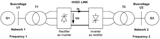 Figure 1. Typical layout of a point-to-point high-voltage direct current (HVDC) power transmission system.
 - Power can be controlled more quickly in HDVC systems than in HVAC systems. For instance, when an imbalance in the AC system (due to any kind of disturbance) is about to occur, the amplitude of the power of the DC line can be changed to counteract and reduce the power oscillations. Therefore, an HVDC link can maintain the specified power flow regardless of severe and dangerous electromechanical oscillations present in the network [3,4]. Improvements in DC voltage measurements at different busbars in different substations have been developed, and DC power flow control is therefore more precise [5,6].
- In HDVC systems, the disturbances are not transferred from one system to another. Therefore, HDVC is very useful in cases where the generation occurs at variable frequency, such as in wind turbines. In addition, meshed AC grids can present problems with high short-circuit currents at times close to the capacity of the installed switchgear with possible current transformers saturation [7]. This situation is solved with the use of HVDC because the link to the nontransferring reactive power does not contribute to the increase in the short-circuit power at the connection node. Furthermore, it has been demonstrated that a good Voltage Source Converter (VSC) control strategy with adequate Proportional Integral (PI) controllers allows a very quick response to disturbances that happen on the AC side [8].
- Although the cost of a HVDC substation is much higher than a HVAC substation, the price per km of line is lower in DC lines. Because DC transmission lines require a smaller number of conductors, the supports and towers are smaller. The width of the street is also smaller and therefore the environmental impact is lower. Consequently, DC transmission lines become economically competitive with the AC ones when the length of the line is several hundred kilometers [9]. Figure 2 shows the dimensions of towers used in AC and DC systems to transport the same power.
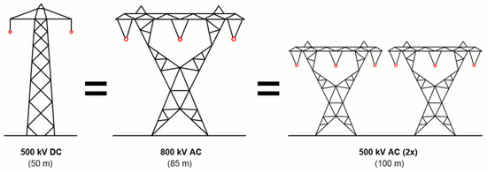 Figure 2. HVDC transmission line versus high-voltage alternating current (HVAC) transmission line.
 - The unlimited use of insulated cable is another advantage of HVDC systems. In AC transmission systems, the cable length is limited due to its ground capacitance. This capacitance involves a capacitive current that is proportional to the cable length so that it can reach the rated cable current at a certain length.
A typical multiterminal HVDC cable networks with four stations and five cables is illustrated in Figure 3.
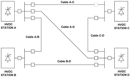
Figure 3.
Multiterminal HVDC system configuration with four stations and five cable lines.
In such a HVDC cable network, when a ground fault happens in any of the cables that connect different HVDC stations, the voltage in the entire system is reduced depending on the severity of the fault and the value of its fault resistance. This situation might lead to the converters disconnecting their semiconductors and causing a collapse in the grid when all HVDC stations are disconnected. Ideally, the correct operation of the protection systems should disconnect only the faulty line, as shown in Figure 4 when there is a ground fault in Cable A–C.
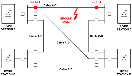
Figure 4.
Multiterminal HVDC selective ground fault protection in case of ground fault in Cable A–C.
It would be convenient to have suitable protection systems that can clear up only the faulty line with full selectivity. For this, the fault currents should be carefully studied. A detailed analysis of the contribution of fault current from the AC side to the DC side under fault conditions in the multiterminal HVDC cable network is presented in Reference [10].
The protection systems currently used in multiterminal HVDC networks use the following methods to detect and clear up faults:
- -
- Analysis of the initial variation of current di/dt: This method uses the behavior of the capacitor on the DC side when a fault happens. A reduced network equivalent is shown in Figure 5. With a fault on the DC network, capacitor C will discharge and therefore add current to the fault. This current contribution depends on the voltage difference between such capacitor and fault position as well as the inductance along the fault circuit.
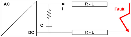 Figure 5. HVDC equivalent network considered for analysis of di/dt HV.
 - -
- Analysis of the rate of current increase: The rate of current increase is used to detect faults mainly due to the very fast increase in the current compared to any other working condition, such as changes in load, switching-off/on maneuvers, etc. The most important advantage of this type of detection is that the fault current is detected a long time before the maximum fault current value is reached. This reduces the instability created by faults in the HVDC network, as well as the breaking capacity for the circuit breakers to be used, to a great extent.
- -
- Analysis of the rate of change of voltage (ROCOV): This method analyses the ROCOV on the line side of the coil erected to limit the di/dt value. The variation in values of the ROCOV is used as quick fault detection in the range of a few microseconds. Different ROCOV values allow the localization of faults with selectivity. ROCOV values decrease significantly as a function of the defect distance to the limiting inductor. The further the fault takes place, the lower is the value of ROCOV. Simulations and research projects have registered values for ROCOV over 30,000 kV/ms when a fault happens close to the limiting inductors and in the range of 1000 kV/ms for faults at distances over 500 km [11].
In this paper, a new differential protection method applied to multiterminal cable networks is introduced. This method measures the currents circulating at the ends of the shields of the insulated cables employed in HVDC networks and applies a differential criterion to determine which cable has a ground defect.
2. State of the Art
HVDC networks are becoming increasingly important in the connection between systems with different frequencies and in the transmission of high active and reactive powers over long distances. Recently, the possible implementation of high-temperature superconducting DC cables has been evaluated [12].
Normally, DC power links are one-to-one type, and the main protections are included in the AC/DC converter on the AC side, although different existing configurations have been evaluated to determine the best possible topology. The selection must evaluate, amongst other parameters, the system losses, transient fault currents, and postfault contingencies. It can be said that there is no DC topology that can meet all aspects [13].
Regarding new HVDC multiterminal networks, more protection functions must be developed in order to grant full selectivity in such grids. These protection systems used in HVDC transmission networks must be at least as fast as the protection devices used in HVAC grids or even faster, mainly because of the quick development of high-fault currents [14,15]. Some applications use the theory of the two-terminal travelling wave [16]. Others research lines have studied short-circuit identification using a wavelet analysis of positive and negative currents in cables to find out the faulty one because the wavelet theory is adequate to analyze transient signals, such as travelling waves, caused by faults [17].
The main differences between HVDC and HVAC protection units are based on the different nature of the short-circuit phenomena. DC fault currents have no zero crossings like AC fault currents. In addition, DC fault currents reach their maximum values in extremely low times, implying very fast rising rates [18]. These two main features of HVDC fault currents force HVDC protections to eliminate faults very quickly—even faster than HVAC—and have driven power converters and the DC circuit breakers to be used applying different fault clearing strategies.
The different options to clear faults at HVDC transmission systems are as follows:
- -
- Switching off the HVAC circuit breakers: This method requires a minimum number of cycles of the AC current signal at rated frequency to detect, identify, and release a tripping command to the corresponding circuit breaker [19]. Unfortunately, this delay time might develop a lack of selectivity in the DC grid. The operation of the AC protection system also implies that the converter in the substation will be out of service. Implementation of converters with blocking options: Some converters can block fault currents [20,21,22] in the time scale of microseconds with consequent improvements in fault clearing time compared to the previous method.
- -
- Use of HVDC circuit breakers: Circuit breakers based on power electronics can switch off fault currents in less than 2 ms but have considerable losses in normal operation [23]. Hybrid HVDC circuit breakers can cut fault currents up to 5 ms with reasonable losses [24,25,26,27]. Another option is the use of mechanical circuit breakers considering breaking times about 10 ms, voltages up to 250 kV, and fault currents with values in the range of 8 kA [28]. The fault current contribution from different sources is absolutely necessary to be well estimated in order to determine the proper ratings of the HVDC circuit breakers [29].
Table 1 illustrates the different time delays in protection relays as well as the cutting-off elements actually used.

Table 1.
Time delays in protection relays and methods of fault current cutting-off.
The measurement and evaluation of voltage change has been recently receiving more attention in HVDC power systems as the principal protection system that detects and clears ground faults in the cables that form such grids [30]. Until now, voltage level protection was generally used as a backup protection. Other backup line protections include DC overvoltage protection and DC line differential protection using optical voltage and current sensors along the cables [31,32]. Indeed, different fault ride-through schemes based on hybrid fault current limiters are now increasingly being considered for multiterminal HVDC networks that connect large-scale offshore wind parks, mainly because these schemes reduce the fault currents and allow mechanical circuit breakers to be used perfectly [33].
3. Proposed Method for Differential Protection of HVDC Cable
The focus of our research is the detection of ground faults in multiterminal DC networks formed by cables. For this, we have introduced a novel differential method for the selective detection of ground faults in DC-insulated cables that have their shields grounded at both ends. The operating principle of the present method is based on the measurement and analysis of the currents that circulate through the ends of the shields of the cables in case of ground fault. The measurements of intensities in shields have important advantages compared to traditional current measurements in active conductors. One advantage is the low cost as there is no necessity for high insulation levels in the measurement sensors. Another advantage is its ease of assembly as current measurement sensors are normally of the ring-core type.
The faulty cable is identified by measuring the polarity of the currents at the ends of the cable shields and comparing such polarities. If the polarities of the currents flowing through the shields are the same, this indicates that the cable has an internal ground fault. However, if the polarities of such currents that circulate through the shields of the protected cable are different, it means that the cable has no ground fault and the ground fault is therefore external.
As can be seen in Figure 6, where an internal ground fault in Stretch 1 is presented, the polarity of the currents at the ends of the shield in Stretch 1 is the same. For the same ground fault, the polarities of the intensities at the respective ends of the shields in Stretches 2 and 3 are different. For an external ground fault outside Stretch 1, as represented in Figure 7, the intensities that circulate at the ends of the shield of Stretch 1 have different polarities. The basic principles of operation of this new method are as follows:
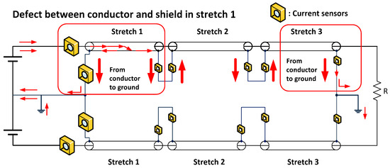
Figure 6.
Current circulation for an internal ground fault in Stretch 1.
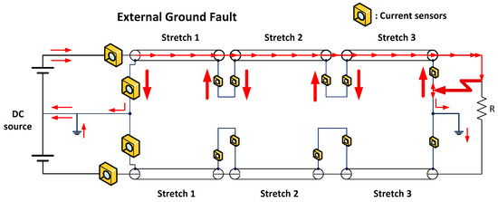
Figure 7.
Current circulation for an external ground fault outside of the cable.
- -
- Measuring of the currents at both ends of cable shield. From these measurements the polarities of the currents can be obtained.
- -
- Internal ground fault in case of same polarities.
- -
- External ground fault in case of different polarities.
This new method is economical as the current sensors used are low-voltage insulated. It is simple to set in operation with easy settings, and it removes the cable with defect from service in a selective way.
4. Simulation Model Implemented in MATLAB Simulink
4.1. Computer Model Description
The model used in MATLAB Simulink (R2011b) considers three different sections of cable—all 100 km in length—with 220 kV as the rated voltage. The technical characteristics of the cable used in the model are given in Table 2 and Table 3.
Table 2.
Main characteristics of 220 kV cable.
Table 3.
Dimensional characteristics of 220 kV cable.
The equivalent PI circuit of this cable considers the mutual impedance between the conductor and the shield as well as the capacitances of conductor–shield and shield–ground. Figure 8 shows such equivalent PI model of the cable.
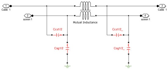
Figure 8.
PI model of the cable used in simulations.
The simulated circuit model is shown in Figure 9. It consists of one Cable A with three cable Stretches 1, 2, and 3; an overhead line with two segments A and B that are 100 km in length each; another Cable B with only one stretch and measuring 100 km in length; two HVDC Stations A and B as sources; a 50 MW load placed at HVDC generation system B; and a fault circuit breaker that allows the ground fault to be placed at any position along the cables or overhead line. The model considers a HVDC system rated 220 kV and loads from 0 to 50 MW connected. Every stretch in Cable A is 100 km in length. At the end of the shields, there are resistance values of 1 mΩ with the purpose of enabling the reading of the currents that circulate through them.
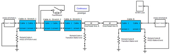
Figure 9.
Model for analysis of the circulations of ground fault currents in shields of power cables.
The parameters of the overhead line are presented in Table 4.
Table 4.
Characteristics of 220 kV overhead line.
4.2. Simulations Results
Numerous ground fault simulations were performed at different locations and with different fault resistance. Some of them are presented as examples, and the results of the simulations are shown in Table 5, Table 6 and Table 7.
Table 5.
Polarities of currents in shields with ground fault in Cable A, Stretch 1. Polarity of currents at the ends of the shields.
Table 6.
Polarities of currents in shields with ground fault in Cable A, Stretch 2. Polarity of currents at the ends of the shields.
Table 7.
Polarities of currents in shields with ground fault in Cable A, Stretch 3. Polarity of currents at ends of the shields.
The currents that circulated in the shield at both ends when a ground fault was simulated in Cable A (Stretch 1) at 25 km from HVDC Station A are shown in Figure 10 and Figure 11.
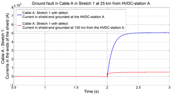
Figure 10.
Circulation of ground fault currents in the ends of the shield in Stretch 1 of Cable A in case of internal ground fault.
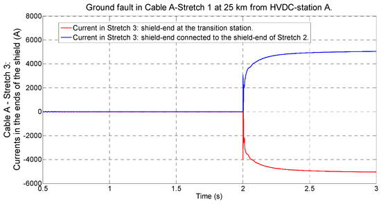
Figure 11.
Circulation of ground fault currents in the ends of the shield in Stretch 3 of Cable A in case of external ground fault in Cable A, Stretch 1.
In Figure 10, it can be seen that the currents in the shield of the faulty conductor occurred when an internal ground fault occurred at time t = 2 s of the simulation. The fault was simulated at a distance of 25 km from the HVDC Station A. Both currents at both ends of such shields had the same polarity.
Figure 11 shows the currents at both ends of the shield of Stretch 3 in Cable A in case of an external ground fault. The currents here had different polarity.
Simulation results with ground faults along the three stretches are given in Table 5, Table 6 and Table 7 considering the system loaded with 50 MW. Different fault resistance values (0, 20, 40, 60, 80, and 100 Ω) were considered at different positions of the ground fault (0, 25, 50, 75, and 100 km) in every stretch in Cable A. Polarities of currents in the shields turned out to be the same when there was no load connected.
According to the simulation results, the differential protection method proposed operated correctly in all cases, i.e., with external and internal faults with several fault resistance levels.
5. Experimental Laboratory Tests and Discussion
5.1. Experimental Set-Up Description
The experimental set-up is illustrated in Figure 12. The laboratory set-up used to validate the simulation results was formed with the following devices:
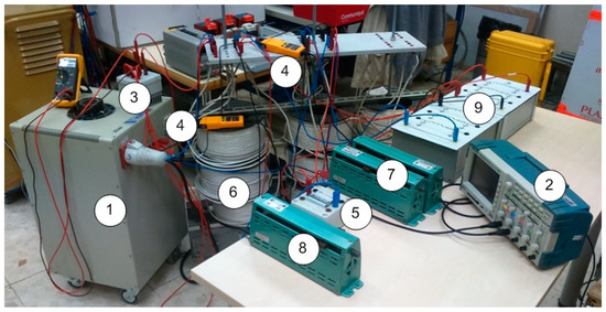
Figure 12.
Experimental set-up. 1: AC power supply; 2: oscilloscope; 3: rectifying bridge; 4: current measurement units; 5: fault switch; 6: cable and shield modules; 7: load resistor; 8: fault resistance; 9: overhead line modules.
- -
- (1) Three-phase AC power supply unit with range of 0–400 Vac/10 kVA.
- -
- (2) Oscilloscope Tektronix TPS2024 with a memory card to save test currents.
- -
- (3) DC-rectifying bridge with input range of 0–480 Vac.
- -
- (4) Clamps FLUKE I30S for measuring currents in the conductor and in its two shield ends with a range of 30 A/sensibility 100 mV/A.
- -
- (5) One circuit breaker to develop ground faults rated 400 V/32 A.
- -
- (6) Three cable sections measuring 100 m in length each. The main characteristics of the cable used were R = 1.8 Ω, L = 22 mH, and C = 4.9 nF with a total cable length of 300 m.
- -
- (7) A load resistor with a range of 0–150 Ω.
- -
- (8) One fault resistance with a range of 0–100 Ω.
- -
- (9) Overhead lines modules included two line modules with equivalent circuit “pi” with R = 88.48 mΩ, L = 4 mH, and C = 4 μF for each capacitor.
The experimental set-up is illustrated in a schematic way in Figure 13.
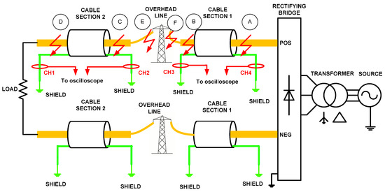
Figure 13.
Layout of experimental ground faults positions in the cable side (A, B, C, and D) and in the overhead line side (F and E).
5.2. Experimental Results
Many ground fault tests were performed on the cable side between positive and shield at positions A, B, C, and D. In addition, ground faults at overhead side were developed in E and F.
Fault resistance ranging from 0 to 100 Ω and resistive loads ranging from 0 to 150 Ω were also considered. The DC voltages used ranged from 50 to 110 Vdc.
Some examples of these tests are presented here. An example of external ground fault is presented in Figure 14, which shows the ground fault currents for a defect with fault resistance of 26 Ω in position F on the overhead line side from positive conductor to ground when the circuit was supplied at 105 Vdc from the DC source and had 1 A load current.
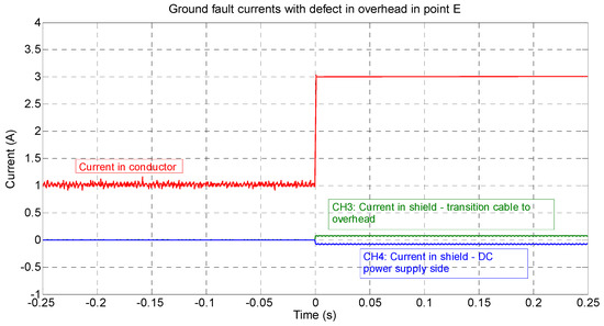
Figure 14.
Ground fault currents with external ground fault in overhead line side in E with 1 A load current.
It can be seen that the currents in the ends of the shield in cable Section 1 had different polarities. This is due to the fact that the fault is outside the cable in the overhead line side.
For faults inside Section 1 and Section 2 of the cable, Table 8 shows the current values read by the sensors CH1, CH2, CH3, and CH4 at the end of the shields when there were faults at points A, B, C, and D in the cable between the positive conductor and shield. Polarities of currents in the shields had the same values when there was no load connected.
Table 8.
Ground fault currents in shield with load connected with test voltage of 105 Vdc.
Table 9 shows the polarity of the currents circulating at both ends of the shields for different ground faults placed at A, B, C, and D. At every end of any shield, currents leaving the shield were considered as positive, and currents entering the shield were considered as negative.
Table 9.
Polarities of ground fault currents in cable without load connected.
Figure 15 shows the currents circulating in the shields of cable Section 1 when a fault happened in cable Section 2. It can be seen that such currents had different polarity.
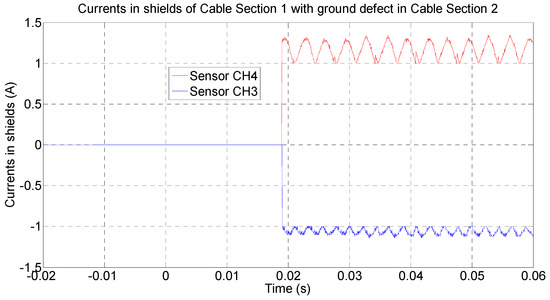
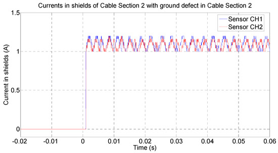
Figure 16 shows the currents circulating in the shields of cable Section 2 when a fault happened in the very same cable. It can be seen that such currents had same polarity, negative in particular, as both currents were leaving the shields to ground. Our reference for currents in shields was negative for currents leaving the shield and positive for currents entering the shield. The results matched this criterion.
5.3. Discussion of Results
The strategy of this novel method described, simulated, and tested in laboratory is the measurement of polarities of the currents that circulate at the ends of the shields of every cable that form a multiterminal HVDC cable network. We developed many tests to check its performance. Ground faults were developed in different singular points as follows:
- -
- Faults between active conductor in the cable and the corresponding shield in points A, B, E, and F (as indicated in Figure 13). Tests developed with voltages 50, 75, and 105 Vdc, fault resistances with 13, 26, 52, and 104 Ω all obtained equal polarities in the currents circulating in the shields from the faulty points to ground at both ends. This shows that the results were totally independent of the voltage level used and the fault resistance values.
- -
- Faults between active conductor and ground at points C and D (as indicated in Figure 13) in the overhead line. Tests with the same voltage levels and fault resistance values employed were identical to those used in points A, B, E and F. Even when the proximity of the faults in the overhead line to the cable line was remarkable, the polarities of the currents circulating in the shields of the cables were different.
Overall, no matter how close the ground fault was to the overhead line side or cable line side, the results were completely satisfactory.
Future research should study the currents that circulate through the cable screens to locate the fault in the cable. New mathematical models, including the variation of such ground resistances, are underway and are aimed at not only finding the cable with defect but the position of the fault as well.
6. Conclusions
A new differential ground fault detection method for DC cables is presented in this paper. The method is based on measuring the current at both ends of the cable shields, which circulate only in case of ground faults. By comparing the polarities of these currents, it can be determined if the ground fault is internal or external, and therefore it is a differential ground fault protection. This technique presents the followings advantages:
- Low installations cost: As the measurement of the currents is performed in the shields, no high voltage sensors are required.
- Easy setting: The operation principle of the protection is the comparison of the polarities of two currents, so no errors in the setting are possible like in other protection functions.
- Suitable for multiterminal HVDC power systems: This new protection is completely selective, so only the cable with internal ground fault will be removed from service. This is an important advantage in comparison to AC protections, which disconnect the AC/DC power converter.
- Long cables with several sections: This technique could be applied to long cables with several sections, and the protection could give information about the faulty section.
The proposed protection method was tested by computer simulations and experimental results with different fault resistances and fault positions and results were successfully obtained.
7. Patents
Granizo Arrabé, Ricardo; Platero Gaona, Carlos Antonio; Blánquez Delgado, Francisco and Rebollo López, Emilio “Metodo y sistema de detección diferencial de defectos a tierra en cables aislados de corriente continua” Spanish Patent ES2524517 12th May 2015.
Author Contributions
Conceptualization, C.A.P.; Methodology, C.A.P.; Software, R.G.A.; Validation, R.G.A. and E.R.L.; Resources, F.A.G.; Writing—Original Draft Preparation, R.G.A., C.A.P., F.A.G., and E.R.L.; Writing—Review and Editing, R.G.A., C.A.P., F.A.G., and E.R.L.; Supervision, C.A.P.
Funding
This research received no external funding.
Conflicts of Interest
The authors declare no conflict of interest.
Abbreviations
The following abbreviations are used in this manuscript:
| AC | Alternating current |
| DC | Direct current |
| HVAC | High-voltage alternating current |
| HVDC | High-voltage direct current |
| IGBT | Insulated-gate bipolar transistor |
| PI | Proportional integral |
| ROCOV | Rate of change of voltage |
| VSC | Voltage source converter |
References
- Jamali, S.; Reza Farsa, A.; Ghaffarzadeh, N. Identification of optimal features for fast and accurate classification of power quality disturbances. Measurement 2018, 116, 565–574. [Google Scholar] [CrossRef]
- Parikh, H.R.; Loeches, R.S.M.; Tsolaridis, G.; Teodorescu, R.; Mathe, L.; Chaudhary, S. Capacitor voltage ripple reduction and arm energy balancing in MMC-HVDC. In Proceedings of the IEEE 16th International Conference on Environment and Electrical Engineering (EEEIC), Florence, Italy, 7–10 June 2016; pp. 1–6. [Google Scholar]
- Udrea, O.; Ungureanu, G.; Lazaroiu, G.C.; Costoiu, M. AC vs. HVDC Back to Back Interconnection cost benefit analysis. In Proceedings of the International Conference on Harmonics and Quality of Power (ICHQP), Bucharest, Romania, 25–28 May 2014; pp. 72–76. [Google Scholar]
- Liu, Y.; Song, W.; Li, N.; Bai, L.; Ji, Y. A Descentralized Optimal Current Sharing Method for Power Line Minimization in MT-HVDC Systems. J. Power Electr. 2016, 16, 2315–2316. [Google Scholar] [CrossRef]
- Feng, P.; Y, X.; Xiao, X.; Xu, K.; Ren, S. Characteristic analysis of shunt for high voltage direct current measurement. Measurement 2012, 45, 597–603. [Google Scholar] [CrossRef]
- Amamra, S.; Colas, F.; Guillaud, X.; Rault, P.; Nguefeu, S. Laboratory Demonstration of a Multiterminal VSC-HVDC Power Grid. IEEE Trans. Power Deliv. 2017, 32, 2339–2349. [Google Scholar] [CrossRef]
- Akbar, A.; Asghar Gholamian, S.; Azari Takami, M.M. A precise scheme for detection of current transformer saturation based on time frequency analysis. Measurement 2016, 94, 692–706. [Google Scholar] [CrossRef]
- Badrkhani, F.; Iravani, R. Dynamic Interactions of the MMC-HVDC Grid and its Host AC System Due to AC-Side Disturbances. IEEE Trans. Power Deliv. 2016, 31, 1289–1298. [Google Scholar] [CrossRef]
- Xiang, X.; Merlin, M.M.C.; Green, T.C. Cost analysis and comparison of HVAC, LFAC and HVDC for offshore wind power connection. In Proceedings of the 12th IET International Conference on AC and DC Power Transmission (ACDC 2016), Beijing, China, 28–29 May 2016; pp. 1–6. [Google Scholar]
- Bucher, M.K.; Franck, C.M. Analytic Approximation of Fault Current Contribution From AC Networks to MTDC Networks During Pole-to-Ground Faults. IEEE Trans. Power Deliv. 2016, 31, 20–27. [Google Scholar] [CrossRef]
- Sneath, J.; Rajapakse, A.D. Fault Detection and Interruption in an Earthed HVDC Grid Using ROCOV and Hybrid DC Breakers. IEEE Trans. Power Deliv. 2016, 31, 973–981. [Google Scholar] [CrossRef]
- Doukas, D.I.; Syrpas, A.; Labridis, D.P. Multiterminal DC Transmission Systems Based on Superconducting Cables Feasibility Study, Modeling, and Control. IEEE Trans. Appl. Supercond. 2018, 28, 5400506. [Google Scholar] [CrossRef]
- Bucher, M.K.; Wiget, R.; Anderson, G.; Franck, C.M. Multiterminal HVDC Networks–What is the Preferred Topology? IEEE Trans. Power Deliv. 2014, 29, 20–27. [Google Scholar] [CrossRef]
- Van Hertem, D.; Ghandhari, M.; Curis, J.B.; Despouys, O.; Marzin, A. Protection requirements for a multi-terminal meshed DC grid. In Proceedings of the Cigrè International Symposium the Electric Power System of the Future Integrating Supergrids and Microgrids Location, Bologna, Italy, 13–15 September 2011. [Google Scholar]
- Adly, A.R.; El Sehiemy, R.A.; Almoataz, Y.; Abdelaziz, A.Y. A novel single end measuring system based fast identification scheme for transmission line faults. Meas. 2017, 103, 263–274. [Google Scholar] [CrossRef]
- Wang, L.; Liu, H.; Dai, L.V.; Liu, Y. Novel Method for Identifying Fault Location of Mixed Lines. Energies 2018, 11, 1529. [Google Scholar] [CrossRef]
- Hossam-Eldin, A.; Lotfy, A.; Elgamal, M. Artificial intelligence-based short-circuit fault identifier for MT-HVDC systems. IET Gener. Trans. Distrib. 2018, 12, 2436–2443. [Google Scholar] [CrossRef]
- Lenz, V.; Schultz, T.; Franck, C.M. Impact of topology and fault current on dimensioning and performance of HVDC circuit breakers. In Proceedings of the 4th International Conference on Electric Power Equipment-Switching Technology (ICEPE-ST), Xi’an, China, 22–25 October 2017; pp. 356–364. [Google Scholar]
- Peng, C.; Husain, I.; Huang, A.Q.; Lequesne, B.; Briggs, R. A Fast Mechanical Switch for Medium-Voltage Hybrid DC and AC Circuit Breakers. IEEE Trans. Ind. Appl. 2016, 52, 2911–2918. [Google Scholar] [CrossRef]
- Schmitt, D.; Wang, Y.; Weyh, T.; Marquardt, R. DC-side fault current management in extended multiterminal-HVDC-grids. In Proceedings of the International Multi-Conference on Systems, Sygnals & Devices, Chemnitz, Germany, 20–23 March 2012; pp. 1–5. [Google Scholar]
- Merlin, M.M.C. The Alternate Arm Converter: A New Hybrid Multilevel Converter With DC-Fault Blocking Capability. IEEE Trans. Power Deliv. 2014, 29, 310–317. [Google Scholar] [CrossRef]
- Xu, Z.; Xiao, H.; Xiao, L.; Zhang, Z. DC Fault Analysis and Clearance Solutions of MMC-HVDC Systems. Energies 2018, 11, 941. [Google Scholar] [CrossRef]
- Bucher, M.K.; Walter, M.M.; Pfeiffer, M.; Franck, C.M. Options for ground fault clearance in HVDC offshore networks. In Proceedings of the IEEE Energy Conversion Congress and Exposition (ECCE), Raleigh, NC, USA, 15–20 September 2012; pp. 2880–2887. [Google Scholar]
- Davidson, C.C.; Whitehouse, R.S.; Barker, C.D.; Dupraz, J.P.; Grieshaber, W. A new ultra-fast HVDC Circuit breaker for meshed DC networks. In Proceedings of the 11th IET International Conference on AC and DC Power Transmission, Birmingham, UK, 10–12 February 2015; pp. 1–7. [Google Scholar]
- Daibo, A. High-speed current interruption performance of hybrid DCCB for HVDC transmission system. In Proceedings of the 4th International Conference on Electric Power Equipment-Switching Technology (ICEPE-ST), Xi’an, China, 22–25 October 2017; pp. 329–332. [Google Scholar]
- Nadeem, M.H.; Zheng, X.; Tai, N.; Gul, M. Identification and Isolation of Faults in Multi-terminal High Voltage DC Networks with Hybrid Circuit Breakers. Energies 2018, 11, 1086. [Google Scholar] [CrossRef]
- Nguyen, V.-V.; Son, H.-I.; Nguyen, T.-T.; Kim, H.-M.; Kim, C.-K. A Novel Topology of Hybrid HVDC Circuit Breaker for VSC-HVDC Application. Energies 2017, 10, 1675. [Google Scholar] [CrossRef]
- Hajian, M.; Zhang, L.; Jovcic, D. DC transmission grid with low speed protection using mechanical DC circuit breakers. IEEE Trans. Power Deliv. 2015, 30, 1383–1391. [Google Scholar] [CrossRef]
- Bucher, M.K.; Franck, C. Contribution of Fault Current Sources in Multiterminal HVDC Cable Networks. IEEE Trans. Power Deliv. 2013, 28, 1796–1803. [Google Scholar] [CrossRef]
- Liu, X.; Osman, A.H.; Malik, O.P. Stationary Wavelet Transform Based HVDC Line Protection. In Proceedings of the 39th North American Power Symposium, Las Cruces, NM, USA, 30 September–2 October 2007; pp. 37–42. [Google Scholar]
- Gang, W.; Min, W.; Haifeng, L.; Chao, H. Transient Based Protection for HVDC Lines Using Wavelet-Multiresolution Signal Decomposition. In Proceedings of the IEEE/PES Transmission & Distribution Conference & Exposition: Asia and Pacific, Dalian, China, 18 August 2005; pp. 1–4. [Google Scholar]
- Tzelepis, D.; Dysko, A.; Fusiek, G.; Nelson, J.; Niewczas, P.; Vozikis, D.; Orr, P.; Gordon, N.; Booth, C.D. Single-Ended Differential Protection in MTDC Networks Using Optical Sensors. IEEE Trans. Power Deliv. 2017, 32, 1605–1615. [Google Scholar] [CrossRef]
- Sanusi, W.; Al Hosani, M.; El Moursi, M.S. A novel Dc fault ride-through scheme for MTDC networks connecting large-scale wind parks. IEEE Trans. Sustain. Energy 2017, 8, 1086–1095. [Google Scholar] [CrossRef]


© 2018 by the authors. Licensee MDPI, Basel, Switzerland. This article is an open access article distributed under the terms and conditions of the Creative Commons Attribution (CC BY) license (http://creativecommons.org/licenses/by/4.0/).