Three-Dimensional Inverse Design of Low Specific Speed Turbine for Energy Recovery in Cooling Tower System

Abstract

A three-dimensional inverse design of a low specific speed turbine is studied, and a set of design criteria for low specific speed turbine runner is proposed, including blade loading distributions and blade lean angles. The characteristics of the loading parameters for low specific speed turbine runner are summarized by analyzing the suction performance of different loading positions, loading slopes and blade lean angles based on the orthogonal experiment design and range analysis. It is found that the blade loading distribution at the band plays a more important role than it does at the crown and it should be fore loaded for both band and crown. The blade lean angle at the blade leading edge should be negative. Then, the blade is optimized through the inverse method by fixing blade lean angle, based on the response surface method. After seeking the optimal value of the response surface function, the optimal result of the design parameters is obtained, which is in conformity with the design criteria and verifies the rationality of the established design criteria for low specific speed turbine.

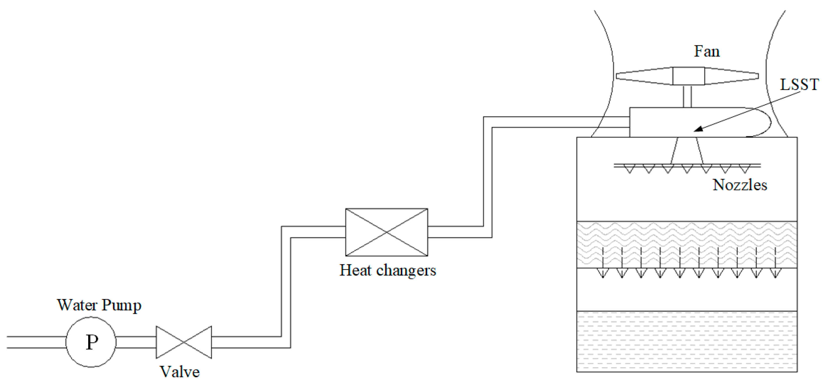
1. Introduction

Cooling towers are widely used to remove heat from industrial processes with heating, ventilating and air conditioning systems. The heat is removed by circulating the water and air through pump and fan respectively, which consume a lot of energy [1,2,3]. After circulation the water has substantial remaining energy to be reused. And a Low Specific Speed Turbine (LSST) is an effective way to save energy for cooling tower system.

The LSST which is applied to drive the fan in cooling tower system (Figure 1) is a typical hydraulic energy recovery device [4,5]. The LSST is used to recover the residual pressure of the circulating water system to drive the fan for energy saving. Typically, the water head is from 5 m to 16 m, the flow range is between 0.06 m³/s and 1.3 m³/s, the rotational speed is from 100 r/min to 250 r/min, and the generating power is generally between 20 kW and 200 kW. Correspondingly, the specific speed of the turbine is within the range of 45 m·kW to 60 m·kW which is far less than the conventional turbines [6]. The main differences between the LSST and the conventional turbines used in hydropower station fall in two aspects. First, the outlet of the LSST is pressurized since it is installed in the circulating water system while the outlet of the conventional turbine is open to surroundings. Therefore, the available water head for LSST associates with not only the surplus pressure of the circulating water system but also with its own characteristics, which will not happen in the conventional turbines. Second, the LSST is used to drive the fan in the cooling tower system rather than electricity generation which is the main concern of the conventional turbines. Hence, the characteristics of the LSST are not only related to its own performances but also related to the characteristics of the fan. Generally, the LSST shows different characteristics with the conventional turbines used in hydraulic power stations [7], which is a main challenge for the hydraulic design of the turbine.

Studies of LSST mainly focus on hydraulic performance and blade geometry [6,7,8,9]. It is found that the hydraulic performance of the LSST is worse than the normal turbines since its working parameters are limited by both the fan and the circulating water system. By optimizing the spiral casing and stay ring the hydraulic loss can be decreased and the efficiency can be increased [7,8], however, there are still differences compared with the normal turbines. More attention should be paid to the design of the impeller since it is the key component for energy conversion.

Compared with the conventional turbine, the blade distortion of the LSST is larger which shows an obvious three-dimensional feature. And it is difficult for the conventional two-dimensional design method to give a satisfactory design result. Moreover, in the conventional two-dimensional design method the design parameters are mainly geometrical and their relationship with the impeller performances are usually not clear. Therefore, the design result depends on the existing experiences which is deficient for the LSST. In order to solve the problem, Borges proposes a three-dimensional inverse design method for turbomachinery [10], which can suppress the secondary flow successfully and improve the performances of the impeller significantly [11]. In the three-dimensional inverse design method, the main design parameters are the blade loading distributions which have direct influence on the hydraulic performances.

The three-dimensional inverse design method has been applied successfully to pump [12], compressor [13], and conventional hydraulic turbine [14,15,16] so far. In the inverse design of a Francis turbine, the loading distribution and the blade stacking condition (blade lean angle) are analyzed and it is found that different blade lean angles can change the pressure distribution on the blade surface, and influence the runner performances [15]. In order to reduce the probability of cavitation, the blade loading at both the band and crown should be fore loaded [14]. Since the flow calculation in the three-dimensional inverse design method is based on potential flow theory with no consideration of the fluid viscosity, simulation with high fidelity [17] is necessary for the design verification. For three-dimensional inverse design method, the blade loading parameters are the most important parameters and a reasonable blade loading distribution can improve the impeller performances significantly.

Compared with conventional hydraulic turbine the LSST shows different characteristics in both performances and blade geometries, since its application conditions are different from the conventional turbines. The design criteria for conventional turbines cannot be applied to the LSST directly. In order to improve the performances of the LSST, a three-dimensional inverse design study of the turbine is conducted. Then a set of design criteria suitable for LSST is summarized. In Section 2 the three-dimensional inverse design method for LSST design and numerical method for performance prediction of the designed LSST are described. Then the blade loading parameters at both the crown and band and the blade lean angle at the blade trailing edge are analyzed in Section 3. And a set of design criteria for the LSST is established. Then an optimization of the LSST is performed to verify the established design criteria. Several conclusions are drawn in Section 4.

2. Materials and Methods

2.1. Three-Dimensional Inverse Design Method

The three-dimensional inverse design method proposed by Borges [10] is adopted. There are two main parts in the inverse design method. One part is the velocity field calculation of the flow based on potential flow theory with no consideration of the fluid viscosity. The other is the blade geometry calculation by applying slip condition of the calculated velocity at the blade surface. The velocity calculation and the blade geometry calculation are performed in an iterative way. The calculations are performed in the meridional flow passage and the key input parameters are the blade loading parameters. The blade loading is defined by drV_q/dm, where r is the radius, V_q is the circumferentially-averaged velocity, and m is the normalization streamline length. The velocity circulation at the turbine inlet is specified according to the Euler formula with zero velocity circulation set at the turbine outlet, which keeps the water head constant during the inverse design calculation.

The blade loading distribution is controlled by a typical “three-segment” curve [16] which consists of two polynomial lines and a straight line between (Figure 2). In the “three-segment” curve, the first intersection point between the polynomial line and the straight line is NC, the second intersection point is ND, and the slope of the middle straight line is defined as the parameter S. When the slope S is greater than zero the maximum of the blade loading will appear in the fore-part of the streamline and it is so called fore-loaded. When the slope S is less than zero the maximum of the blade loading will appear in the aft-part of the streamline and it is so called aft-loaded. The subscript C represents the crown, while the subscript B represents the band hereafter. The blade loading distribution is controlled by the two streamlines at both the crown and the band. The blade loading distributions between the two streamlines are determined by linear interpolation.

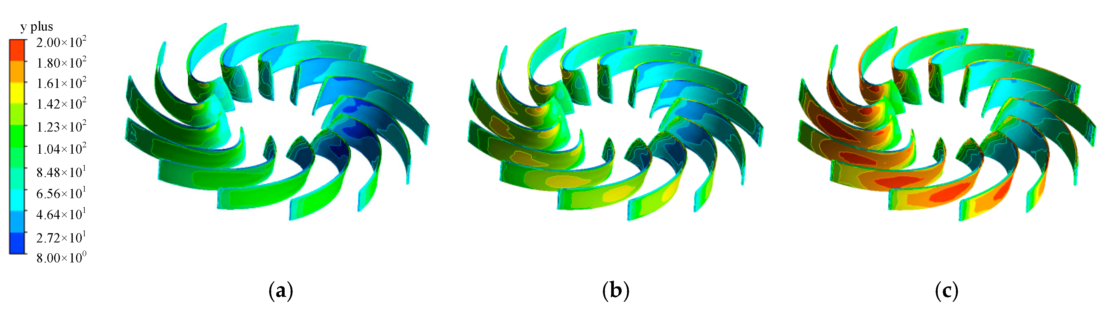
2.2. Numerical Method

The numerical simulation is applied to evaluate the steady performances of the LSST for design parameters comparison. The specific speed ns of the LSST studied is about 47 according to

$$n_s=\frac{n\sqrt{P}}{H^{5/4}}$$

(1)

where n_s is the specific speed, n is the revolution speed in rpm, P is the power in kW, and H is the working head in m. The number of the runner blade is 13, the number of the guide vane blade is 20 and the cone angle of the tailpipe is 12°. The computational domain is depicted in Figure 3, while the meridian passage of the runner is shown in Figure 4.

SSTk–ω turbulence model with standard wall function is applied for steady performance evaluation. A total pressure calculated from water head is set at the inlet and a zero static pressure is set at the outlet. No-slip boundary condition is set at all the walls. The second order difference scheme is used to solve the steady equations. The commercial code of ANSYS CFX (15.0, ANSYS Company, Cannonsburg, PA, USA) was applied to conduct the numerical simulations. All the steady simulations were converged by setting the residual values of 10⁻⁴ for the simulated variables. The space discretization was based on a cell-centered finite volume scheme with the system of governing equations. A frozen rotor model was used for the present domain including both stationary and rotation parts. And a SIMPLEC algorithm was applied to the solution of pressure and velocity.

For wall bounded turbulence flow the near wall mesh treatment is important, since the near-wall velocity simulation plays an important role in the correct interpretations of turbulence data [18]. In the present simulation three sets of mesh with different wall mesh treatment are compared. The y plus (normal to the blade surface) distributions at the blade surface of the three mesh are shown in Figure 5. Since the standard wall function is applied the y plus near the wall should be between 30 and 300 and all the three mesh are qualified. Here the mesh with 3.21 million cells in total with maximum y plus of 113 is set as the final case since it has the smallest value of averaged y plus. In addition to y plus the value of both the x plus (tangential to the blade surface) and z plus of the blade are no more than 250, specifically, the grid spacing in z direction is less than the half of that in x direction since turbulent structures are elongated in the streamwise direction.

3. Design Parameter Analysis

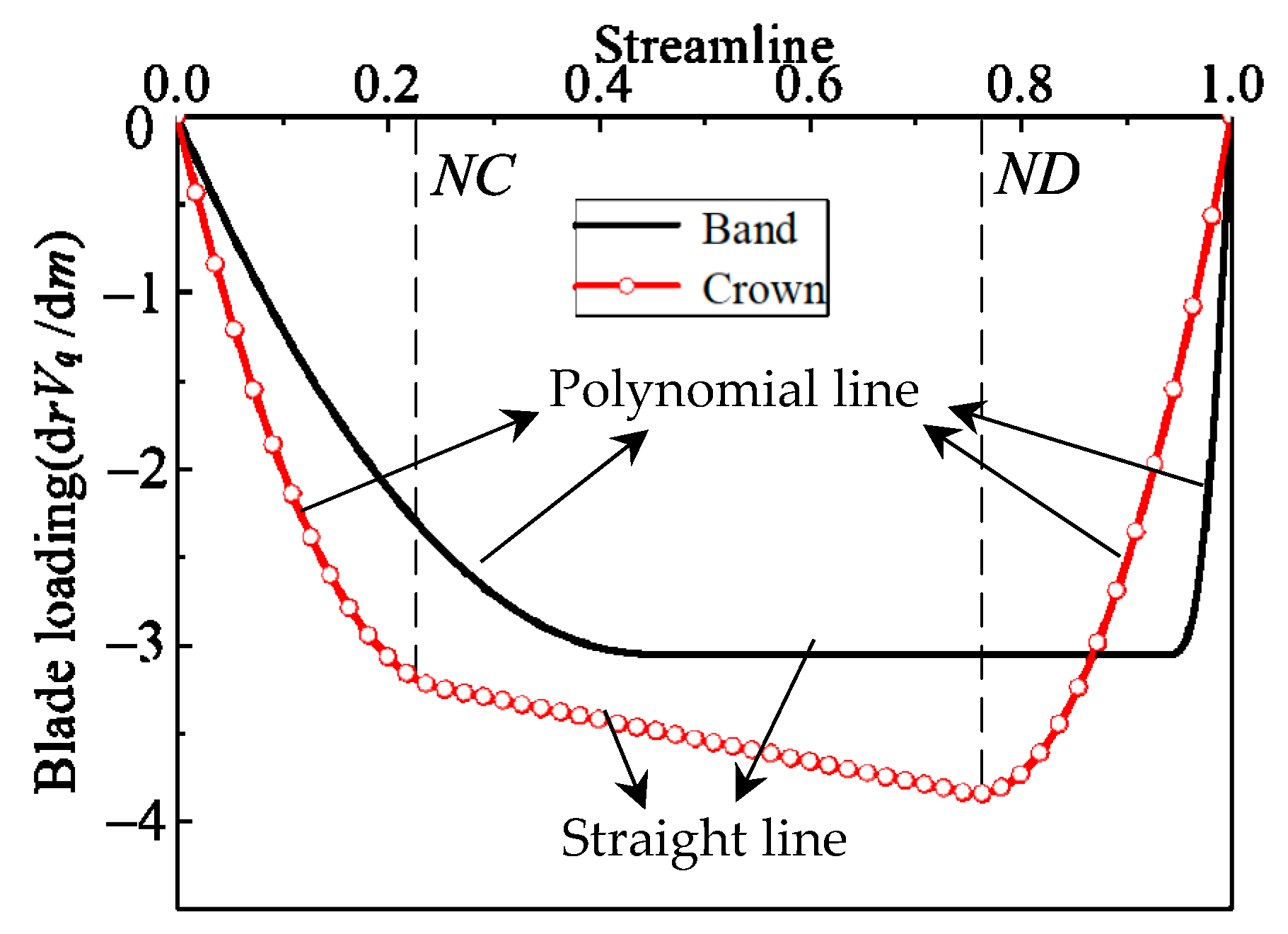
3.1. Blade Loading Parameters

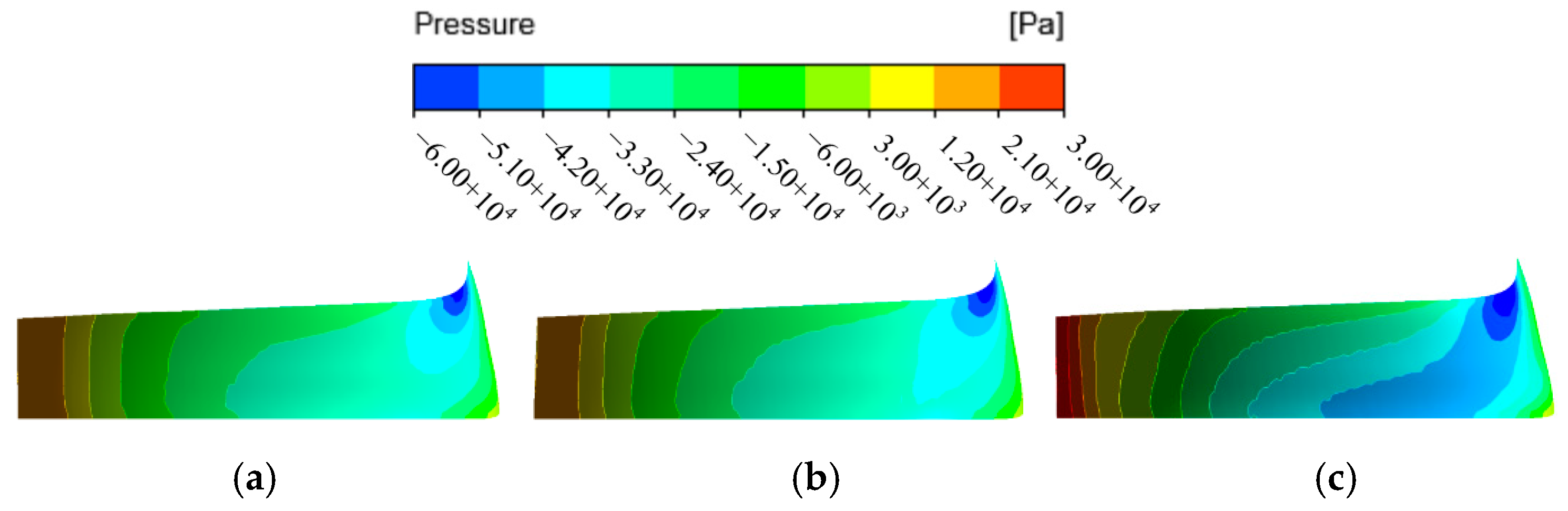
3.1.1. The After-Loading Point at the Band

Selecting three typical values for the after-loading point at the band: 0.55, 0.75, 0.95, while the other parameters are fixed. As depicted in Figure 6, the pressure of the suction surface gradually decreases and the area of the low-pressure region increases with the after-loading point moving backward. The pressure at the band near trailing edge is lower and the low-pressure area is larger. And the low-pressure area at the middle of the crown develops from nothing. Thus, the pressure gradient between the band and the crown increases, which gives the chance to the secondary flow development [11]. The lower the ND_B is the smaller the low-pressure area is.

When the after-loading point at the band is between 0.75 and 0.95 for mid-loaded or after-loaded blade, the pressure on the suction surface spreads unevenly, which extends to the outlet and leads to an obvious low speed zone as shown in Figure 7. To sum up, should be between 0.55 and 0.75 to get better flow performance with reasonable pressure and velocity distributions.

3.1.2. The Front-Loading Point at the Band

Selecting three typical values for the front-loading point at the band: 0.05, 0.25, 0.45, while the other parameters are fixed. As depicted in Figure 8, there is an obvious area of low-pressure region on the suction surface when the front-loading point picks the value of 0.45, while the pressure is more uniform when $N{C}_{\mathrm{B}}$ is between 0.05 and 0.25.

3.1.3. The Front-Loading Point at the Crown

Based on plenty of numerical experiments, the front-loading point at the crown NC_c has little influence on the pressure of the suction surface that it is difficult to figure out the distinctions between different NC_c values in the static pressure distributions. Figure 9 shows the static pressure coefficients Cp with NC_c equaling to 0.05 and 0.45 while ND_c is fixed to 0.75. The pressure varies little near the band, while at the crown, the lowest point is slightly lower for NC_c equaling to 0.45 than to 0.05.

3.1.4. The After-Loading Point at the Crown

Selecting three typical values for the after-loading point at the crown ND_c: 0.55, 0.75, 0.95, while the other parameters are fixed. As is depicted in Figure 10, the pressure of the suction surface gradually decreases and the low-pressure area at the band near trailing edge increases with the after-loading point moving backward, while the pressure near the leading edge becomes nonuniform which might lead to the secondary flow. Consequently, ND_c should be set between 0.55 and 0.75, and it is better near 0.55 since it has a more uniform pressure distribution as shown in Figure 9a.

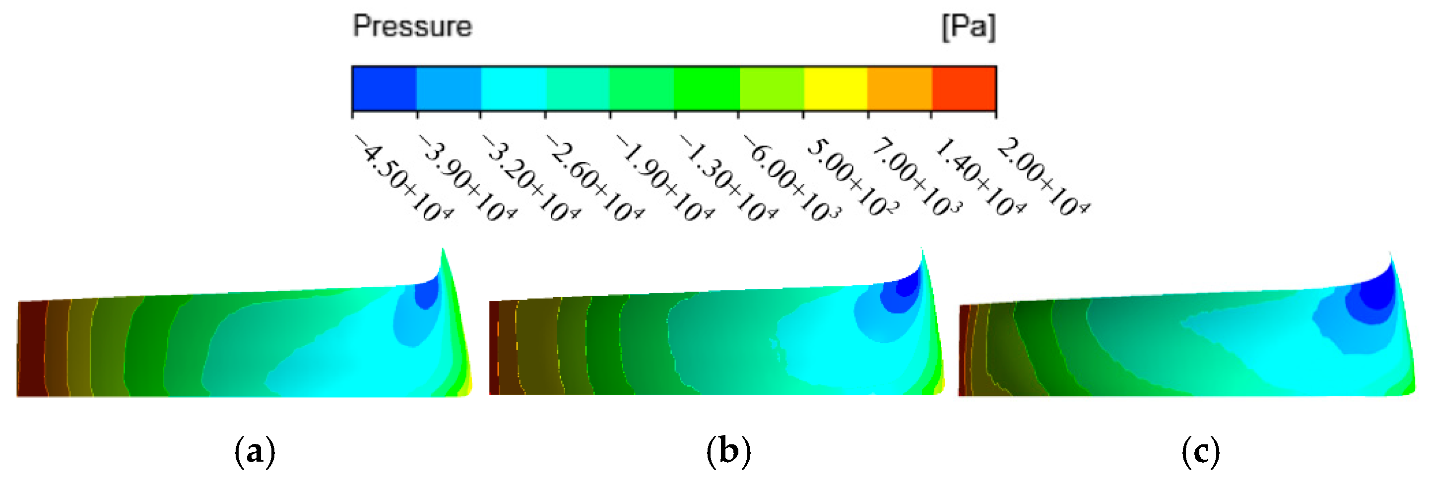
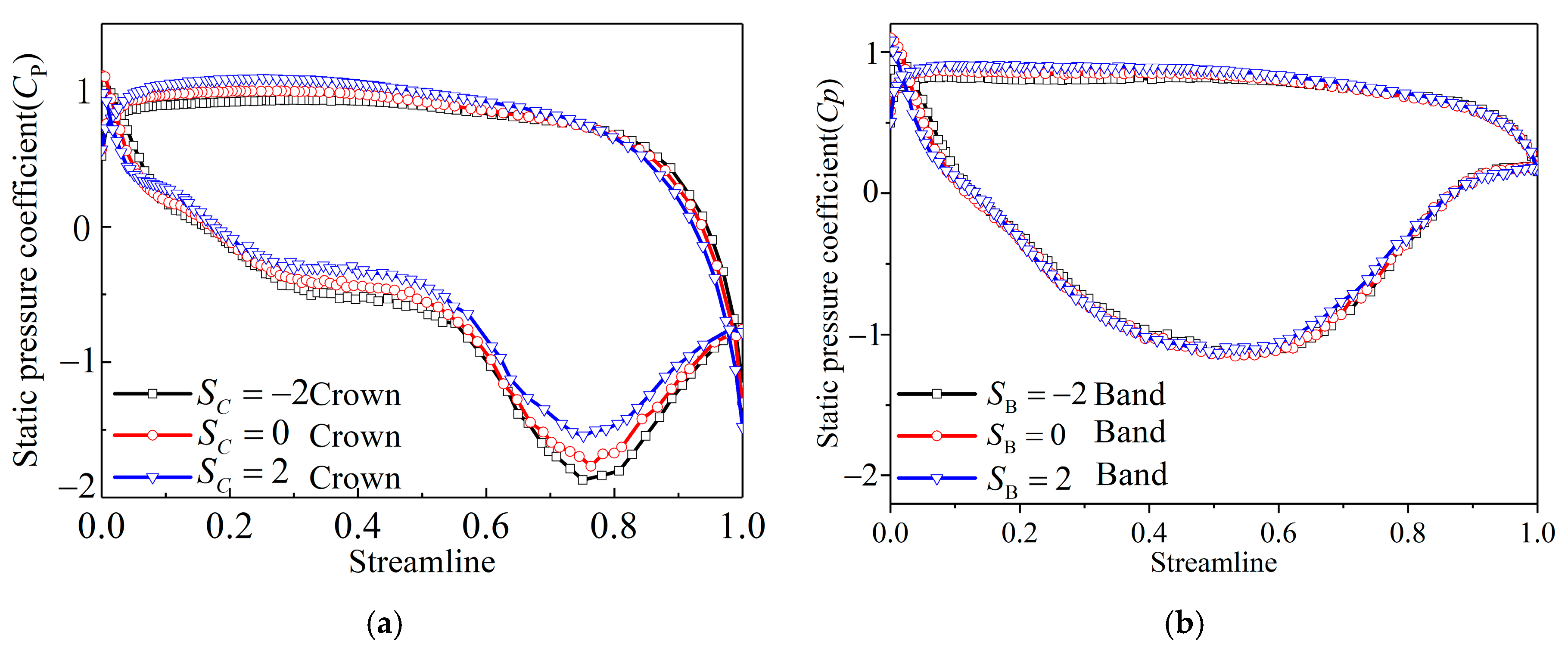
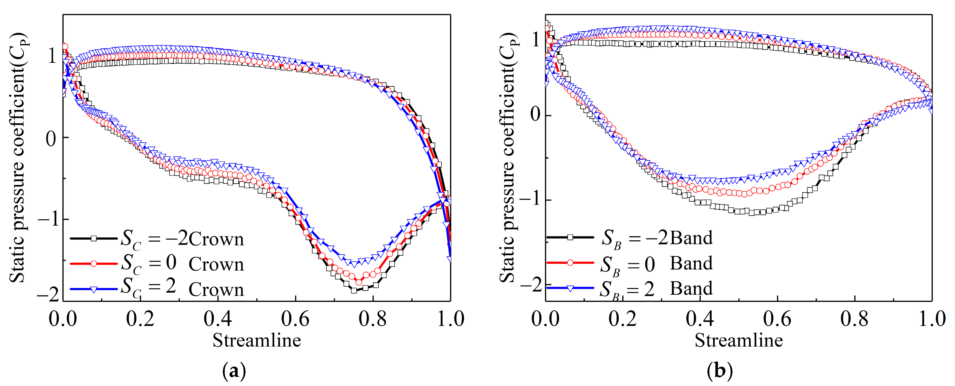
3.1.5. The Slope of the Blade Loading Distribution

The slope of the blade loading distribution S determines the loading type of the blade, which plays an important role in the blade loading design. There are three typical blade loading types for turbine. The main loading point is the after loading point when the slope of the blade loading S is negative, which is called aft-loaded. Conversely, it is fore loaded for the positive S and central loaded for S set to 0. As shown in

Table 1. Loading parameter values with different blade loading slope (NC and ND are the first and second interaction point between the straight line and the parabolic line respectively. S_B and S_C are the slope of the straight line at band and crown respectively).

Number	NC	ND	SB	SC
1	0.05	0.55	−2	−2
2	0.05	0.55	−2	0
3	0.05	0.55	−2	2
4	0.05	0.55	0	0
5	0.05	0.55	2	0

, five runners with the same NC and ND value and different blade loading slope S are designed and analyzed to discuss the effect of the parameter S on the turbine performances.

Comparing the runner number 1, 2 and 3 with different blade loading slope at the crown S_C, the pressure varies little near the band, while at the crown, the minimum pressure point decreases when the loading type turns from fore-loaded to aft-loaded with decrease of S_C. Fore-loaded blade loading with positive S_C, is beneficial to reduce the low-pressure area as shown in Figure 11a.

Comparing the runner number 3, 4 and 5 with different blade loading slope at the band S_B, the pressure is lower for both the band and the crown when the blade loading is aft-loaded with negative S_B. It can be shown in Figure 12b that S_B should be positive to reduce the probability of cavitation, which means the band is better to be fore loaded.

3.1.6. Parameter Priority Analysis

In order to analyze the blade loading parameter priority a sample space of the above six blade loading parameters with three levels of each parameter was set for an orthogonal test. Picking up the $L_{36}\left(3^6\right)$ orthogonal table, the parameters with three levels are shown in

Table 2. Six blade loading parameters with three levels for the orthogonal test.

Parameters	NCB	NDB	SB	NCC	NDC	SC
Level 1	0.05	0.55	−2	0.05	0.55	−2
Level 2	0.25	0.75	0	0.25	0.75	0
Level 3	0.45	0.95	2	0.45	0.95	2

.

By range analysis, the influence of various parameters and levels on the turbine efficiency was analyzed.

Table 3. Range analysis of the orthogonal test results.

Efficiency	NCB	NDB	SB	NCC	NDC	SC
$T_1$	1111.93	1109.28	1090.34	1107.08	1104.02	1098.19
$T_2$	1098.95	1101.85	1101.45	1098.61	1101.96	1099.52
$T_3$	1090.42	1090.17	1109.51	1095.60	1095.32	1103.58
${\overline{T}}_1$	92.66	92.44	90.86	92.26	92.00	91.52
${\overline{T}}_2$	91.58	91.82	91.79	91.55	91.83	91.63
${\overline{T}}_3$	90.87	90.85	92.46	91.30	91.28	91.97
$R$	1.79	1.59	1.60	0.96	0.72	0.45

shows the results of the range analysis, in which T_i is the summation of the turbine efficiency under the same parameter level, ${\overline{T}}_i$ is the averaged turbine efficiency under the same parameter level, R is the range between the maximum ${\overline{T}}_i$ and minimum ${\overline{T}}_i$, where i = 1, 2, 3 means the three levels. All the turbine efficiency mentioned in Table 1 was multiplied by 100 times. Based on orthogonal test and range analysis larger R means more influence of the parameters. It can be found that blade loading at the band plays a more important role than the blade loading at the crown. Specially the front-loading point at the band NC_B shows the greatest influence while the blade loading slope at the crown S_C shows the minimal impact. As a result, for LSST design more considerations should be taken on the blade loading distribution at the band.

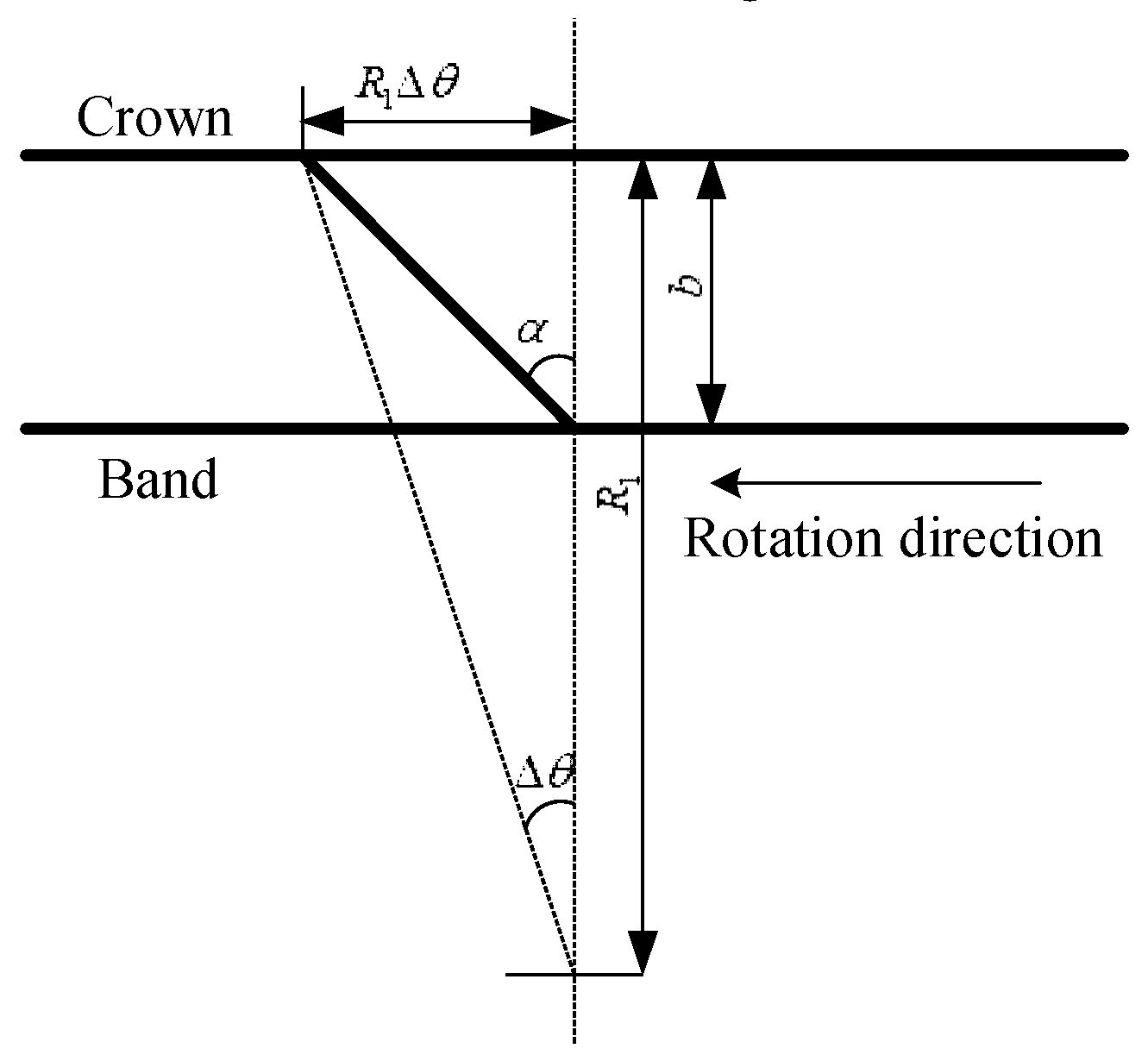
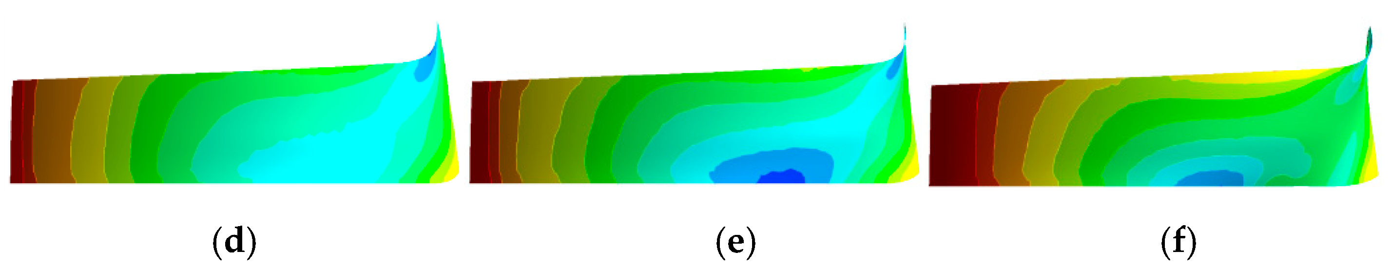
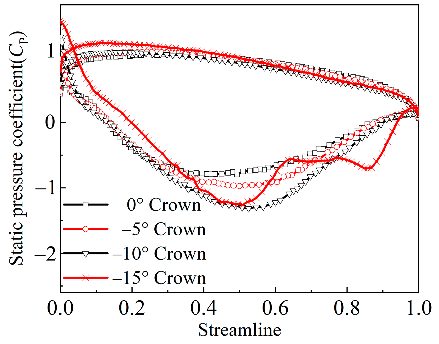
3.2. Blade Lean Angle at Leading Edge

In the three-dimensional inverse design method, the stacking condition is related to the blade lean angle. The stacking condition contains two parameters: the stacking angle and the stacking location. As shown in Figure 13, the relationship between the stacking angle and the blade lean angle is as follows:

$$\alpha =-{\tan }^{-1}(R_1\Delta \theta /b)$$

(2)

where α is the blade lean angle, $\Delta \theta$ is the stacking angle, $R_1$ is the diameter of the crown, and b is the blade width.

The following study on stacking condition was set with different blade lean angles and fixed stacking location at the leading edge. In order to simplify the analysis below, the following blade lean angles is taken as $\Delta \theta$ rather than $\alpha$ shown in Figure 13.

The blade lean angles are set as 10°, 5°, 0°, −5°, −10° and −15° respectively based on the computational convergence, where the minus sign means the blade at the band is ahead of it at the crown in the rotation direction. Six runners with the above blade lean angles were designed, and the effect of the blade lean angles on the performance of the runner was compared and analyzed. As shown in Figure 14, the pressure of the suction surface with different blade lean angles are compared. For the runner with blade lean angles of 0°, 5° and 10°, the pressure near the band decreases when the blade lean angle increases, which may lead to cavitation near the band. Meanwhile, the low-pressure region moves from the band towards the crown with the decrease of the blade lean angles. For the runner with blade lean angles of 0°, −5°, −10° and −15°, the blade pressure becomes more ununiform when the blade lean angle picks the value of −10° and −15°.

Runner with blade lean angles of 0°, −5°, −10°and −15° are shown in Figure 15, in which the suction surface pressure decreases from 0° to −10°. And when the blade lean angle is −15°, the pressure fluctuates strongly in the middle and posterior parts, which lead to an obvious lower speed zone at the runner outlet compared with the runner with blade lean angle of 0° (Figure 16).

The following design criteria for LSST can be derived based on the above parameter analysis:

(1)

For blade loading design parameters, more attention should be payed to the loading distribution at the band and both the band and crown should be fore loaded.

(2)

For blade lean angles at the leading edge, negative values of the blade lean angles are suggested and the specific values should be within 0° and −5°.

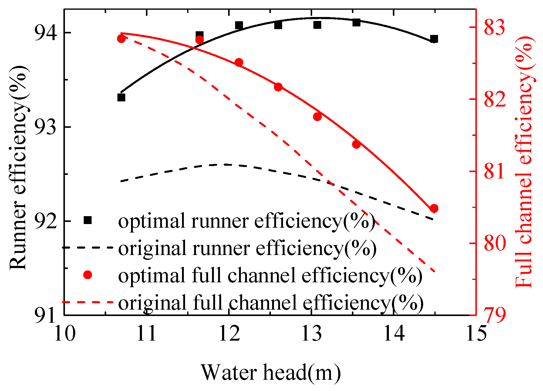
3.3. Verification of the Design Criteria

In order to verify the established design criteria an optimization of the LSST runner was conducted based on a response surface method. The optimization result was obtained by fitting the response surface function of the 36 sets of data based on the orthogonal experiment of the blade loading parameters. The second-order response surface function is defined as follows:

$$y={\beta }_0+\sum _{i=0}^6{\beta }_i{x}_i+\sum _{i=0}^6{\beta }_{ii}{x}_i^2+\sum _{\begin{array}{c}i=1\\ j=1\\ i\ne j\end{array}}^6{\beta }_{i,i}{x}_i{x}_j$$

(3)

where $y$ is the hydraulic efficiency which is the optimal objective, $x_i$ is the value of different levels for each design parameters, ${\beta }_i$ is the undetermined coefficients. The number of the design parameters is 6, and the number of the coefficients is 28. The 28 coefficients are determined by 36 groups of numerical experiments based on the response surface function fitted by the least-square method. After the response surface function was obtained a simulated annealing algorithm was used to find the global optimal solution. The simulated annealing algorithm is a gradient-free optimization method such as genetic algorithm which can also be applied to the present optimization. The optimization result is shown in

Table 4. Optimization of response surface function.

NCB	NDB	SlopeB	NCC	NDC	SlopeC
0.05	0.55	2	0.05	0.596	1.3356

.

The runner efficiency in Figure 17 is defined as

$${\eta }_r=\frac{M\omega }{\rho gQH}=\frac{M\omega }{Q(P_{\mathrm{in}}-P_{\mathrm{out}})}$$

(4)

where M is the torque of the runner, ω is the angular velocity of the runner, ρ is the density of the water, g is the gravitational acceleration, H is the water head defined by (P_in − P_out)/ρg, Q is the flow rate of the turbine, P_in and P_out are the total pressure at the inlet and outlet of the runner respectively. The full channel efficiency is defined as the same way with the P_in and P_out replaced with the total pressure at the turbine inlet and outlet respectively. It can be found that both the runner efficiency and full channel efficiency of the optimized turbine based on Table 4 is apparently higher than the original one. After optimization the efficiency difference between the runner is bigger than the full channel, which means a better result can be obtained by full channel optimization. The values listed in Table 4 are within the range of the above design parameter analysis, which verifies the established design criteria.

4. Conclusions

The influence of different blade loading parameters and blade lean angles on the performance of a LSST runner is studied based on the three-dimensional inverse design method. CFD (Computational Fluid Dynamics) technique is applied to compare the performance of the designed LSST. The blade loading parameter priority at both the band and crown is analyzed based on orthogonal experiment design and range analysis. Then a set of design criteria of the LSST is proposed:

(1)

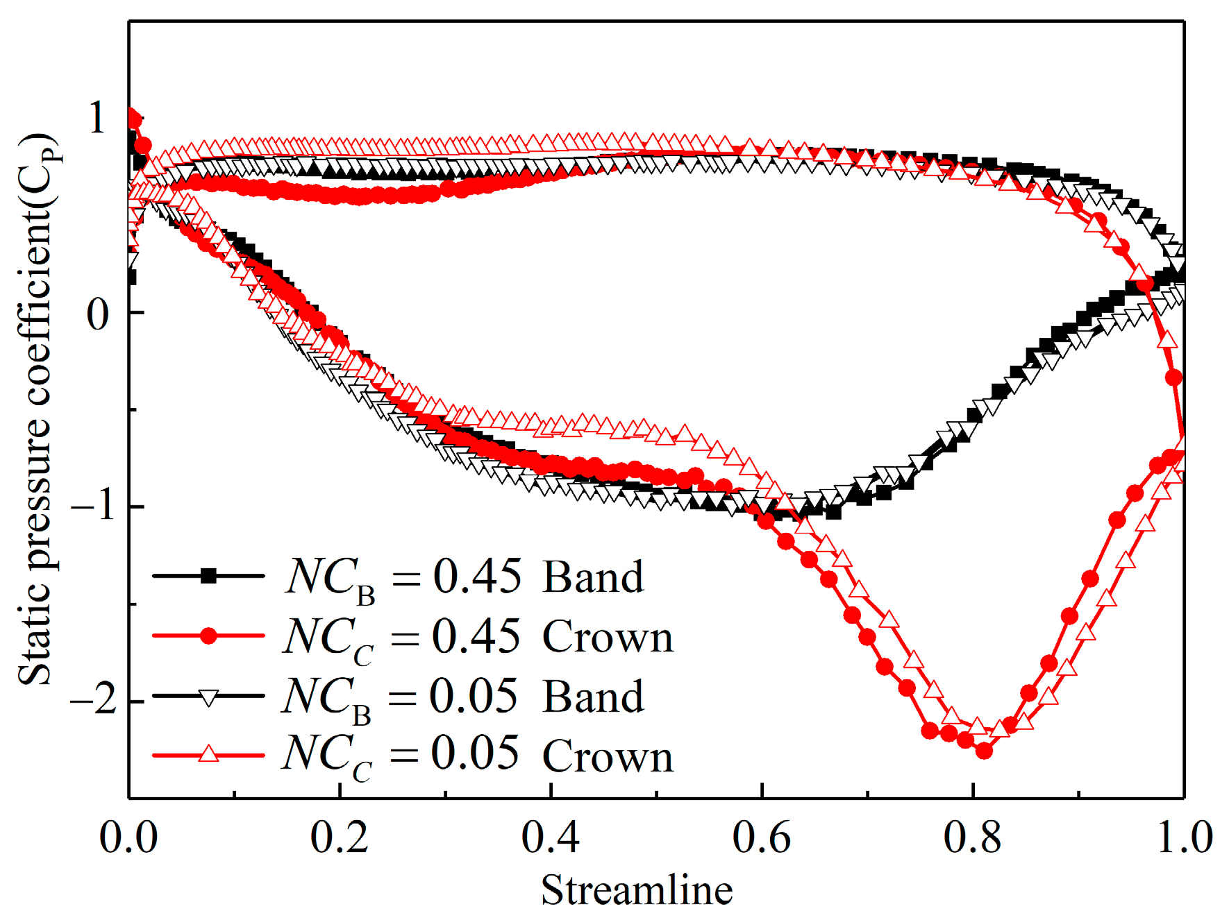
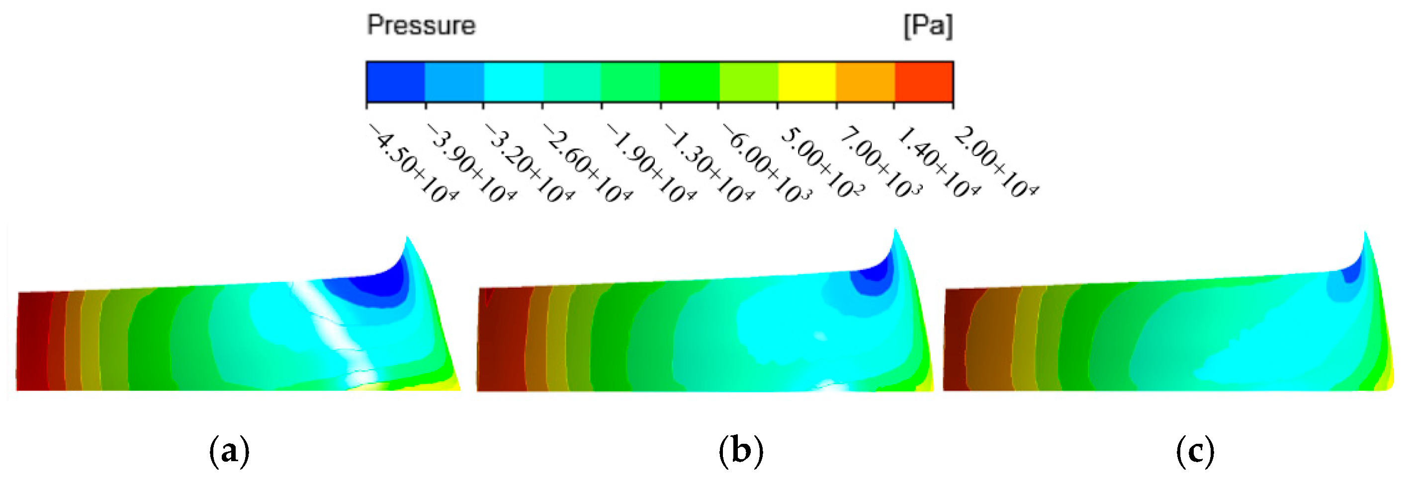
The blade loading parameters at the band have greater effect than the crown. And the most essential parameter is the front-loading point at the band. Both the band and crown should be fore loaded, which is beneficial to a more uniform pressure distribution and a better cavitation performance.

(2)

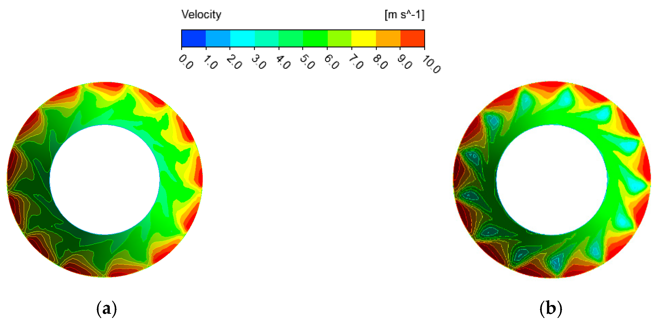
The blade lean angle at the leading edge of the blade should be negative, which means the blade at the band is ahead of it at the crown in the rotation direction. Specifically, the blade lean angle at the leading edge of the blade should be within 0° and −5° for the studied LSST.

Finally, an optimization design based on the response surface method is conducted and the optimization results show that both the runner efficiency and the full channel efficiency of the optimized turbine are higher than the original turbine. The efficiency difference between the runner is greater than the full channel indicating that a better result may be achieved through the full channel optimization. Generally, the runner optimization results are consistent with the blade loading parameter analysis, which verifies the established design criteria for hydraulic design of the LSST.

References

- Goshayshi, H.R.; Missenden, J.F.; Tozer, R. Cooling Tower—An Energy Conservation Resource. Appl. Therm. Eng. 1999, 11, 1223–1235. [Google Scholar] [CrossRef]
- Guang, Y.J.; Wen, J.C.; Lu, L.; Eng, L.L.; Andrew, C. A Simplified Modeling of Mechanical Cooling Tower for Control and Optimization of HVAC Systems. Energy Convers. Manag. 2007, 2, 355–365. [Google Scholar]
- Zhang, H.C.; Fang, L.; Guang, H.; Niu, Y. Review on Water Distribution of Cooling Tower in Power Station. In IOP Conference Series: Earth and Environmental Science; IOP: Sanya, China, 2018. [Google Scholar]
- Singh, R.; Cabibbo, S. Hydraulic Turbine Energy Recovery-R.O. System. Desalination 1980, 32, 281–296. [Google Scholar] [CrossRef]
- Gopalakrishnan, S. Power Recovery Turbines for the Process Industry. Pump Symposium, 1st ed.; Texas A & M University: College Station, TX, USA, 1986. [Google Scholar]
- Li, Y.P.; Nan, H.P.; Duan, K.C. Determination of Key Technical Parameters of Special Hydraulic Turbine for Cooling Tower. Manuf. Sci. Technol. 2012, 383, 1386–1390. [Google Scholar] [CrossRef]
- Zhang, L.J.; Wang, L.; Ren, Y. Characteristic Analysis of Francis-Turbine in Cooling Tower. Appl. Mech. Mater. 2012, 190, 57–59. [Google Scholar] [CrossRef]
- Zhang, L.J.; Ren, Y.; Li, Y.P.; Chen, D.X. Hydraulic Characteristic of Cooling Tower Francis Turbine with Different Spiral Casing and Stay Ring. Energy Procedia 2012, 16, 651–655. [Google Scholar] [CrossRef]
- Li, Y.P.; Ma, J.P.; Chen, D.X. Work Characteristics and Type Selection of Special Turbine in Hydrodynamic Cooling Tower. Appl. Mech. Mater. 2011, 48, 1368–1371. [Google Scholar] [CrossRef]
- Boeges, J.E. A Three-Dimensional Inverse Method for Turbomachinery: Part I—Theory. J. Turbomach. 1990, 3, 346–354. [Google Scholar]
- Zangeneh, M.; Goto, A.; Harada, H. On the Design Criteria for Suppression of Secondary Flows in Centrifugal and Mixed Flow Impellers. J. Turbomach. 1998, 4, 723–735. [Google Scholar] [CrossRef]
- Goto, A.; Zangeneh, M. Hydrodynamic Design of Pump Diffuser Using Inverse Design Method and CFD. J. Fluids Eng. 2002, 2, 319–328. [Google Scholar] [CrossRef]
- Bonaiuti, D. On the Coupling of Inverse Design and Optimization Techniques for the Multiobjective, Multipoint Design of Turbomachinery Blades. J. Turbomach. 2009, 131, 1–16. [Google Scholar] [CrossRef]
- Okamoto, H.; Goto, A. Suppression of Cavitation in a Francis Turbine Runner Using 3D Inverse Design Method. In Proceedings of the 2002 Joint US ASME-European Fluids Engineering Summer Conference, Montreal, WI, USA, 14–18 July 2002. [Google Scholar]
- Daneshkah, K.; Zangeneh, M. Parametric Design of a Francis Turbine Runner by Means of a Three-Dimensional Inverse Design Method. In Proceedings of the 25th IAHR Symposium on Hydraulic Machinery and Systems, Timişoara, Romania, 20–24 September 2010. [Google Scholar]
- Yang, W.; Xiao, R.F. Multiobjective Optimization Design of a Pump–Turbine Impeller Based on an Inverse Design Using a Combination Optimization Strategy. J. Fluids Eng. 2013, 136, 014501. [Google Scholar] [CrossRef]
- Vinuesa, R.; Hosseini, S.M.; Hanifi, A.; Henningson, D.S.; Schlatter, P. Pressure-Gradient Turbulent Boundary Layers Developing around a Wing Section. Flow Turbul. Combust. 2017, 99, 613–641. [Google Scholar] [CrossRef] [PubMed]
- Vinuesa, R.; Nagib, H.M. Enhancing the Accuracy of Measurement Techniques in High Reynolds Number Turbulent Boundary Layers for More Representative Comparison to Their Canonical Representations. Eur. J. Mech. B/Fluids 2016, 55, 300–312. [Google Scholar] [CrossRef]