Article

Energy Uncertainty Analysis of Electric Buses

1
Department of Mechanical Engineering, School of Engineering, Aalto University, Puumiehenkuja 5, 02150 Espoo, Finland
2
Department of Agricultural Sciences, University of Helsinki, Koetilantie 5, 00014 Helsinki, Finland
*
Author to whom correspondence should be addressed.
Energies 2018, 11(12), 3267; https://doi.org/10.3390/en11123267
Submission received: 5 July 2018 / Revised: 26 October 2018 / Accepted: 16 November 2018 / Published: 23 November 2018

Abstract

:
Uncertainty in operation factors, such as the weather and driving behavior, makes it difficult to accurately predict the energy consumption of electric buses. As the consumption varies, the dimensioning of the battery capacity and charging systems is challenging and requires a dedicated decision-making process. To investigate the impact of uncertainty, six electric buses were measured in three routes with an Internet of Things (IoT) system from February 2016 to December 2017 in southern Finland in real operation conditions. The measurement results were thoroughly analyzed and the operation factors that caused variation in the energy consumption and internal resistance of the battery were studied in detail. The average energy consumption was 0.78 kWh/km and the consumption varied by more than 1 kWh/km between trips. Furthermore, consumption was 15% lower on a suburban route than on city routes. The energy consumption was mostly influenced by the ambient temperature, driving behavior, and route characteristics. The internal resistance varied mainly as a result of changes in the battery temperature and charging current. The energy consumption was predicted with above 75% accuracy with a linear model. The operation factors were correlated and a novel second-order normalization method was introduced to improve the interpretation of the results. The presented models and analyses can be integrated to powertrain and charging system design, as well as schedule planning.

1. Introduction

Battery electric buses (BEBs) have recently emerged as an environmentally friendly, yet expensive alternative for diesel buses [1]. In addition to the high initial investment, the life cycle costs (LCC) depend on the selected charging strategy (e.g., overnight vs. opportunity charging) and the selected battery capacity that is defined by the charging strategy [2]. However, the energy consumption rate (ECR) varies because of uncertainties in weather and driving behavior [3]. Variation in ECR may cause delays in the charging schedules, which are hard to predict, because such delays have not been an issue with diesel buses. On the other hand, overly conservative schedules could lead to underutilization of the bus fleet and higher ticket prices. Therefore, the sensitivity of ECR and charging efficiency require detailed investigation with real-world data to ease the transition to fully electric public transportation.
The sensitivity of ECR has been studied previously with analytical models [4,5]. These studies focused on light-duty electric vehicles (EV) and indicated that the drive efficiency, tire losses, acceleration jerks, and auxiliary devices caused the most variation in consumption. Auxiliary devices included heating, ventilation, and air conditioning (HVAC) devices. Furthermore, the effects of mild elevation profile and average speed over 20 km/h were negligible. However, even though hilly roads significantly increased the ECR of EVs, they have an advantage over diesel-powered vehicles because of regenerative braking [6]. In studies that included real-world measurements of EVs, the route, ambient temperature, and driving behavior have been shown to increase ECR [7,8,9]. Lorf et al. [10] noted that traction ratio—the ratio of how much of the driving time is spent on acceleration—caused 23% of the ECR variation of an EV. Younes et al. [8] reported that ECR is also higher for EVs on city routes, as a result of more frequent stop-and-go driving, yet they did not consider the effect of ambient temperature.

2. State-of-the-Art

Unlike EVs, city buses operate on predetermined routes and the number of stops on route is defined by vehicle and passenger traffic. Lajunen & Kalttonen [11] simulated that driving aggressiveness was related to the bus route and was linked to ECR. Lajunen [12] also developed a method for optimizing the speed profile of BEBs, which improved energy efficiency by up to 17%. In addition to bus payload, a notable consumption and consumption variation difference between lightweight (0.52–1.42 kWh/km [13,14]) and heavyweight chassis buses (1.24–2.48 kWh/km [15]) has been reported. During the years 2014–2015, Kontou & Miles [16] tested a BEB fleet of eight buses in Milton Keynes, GB. One of their key findings was that some of the 46 drivers were very consistent and others had variation of up to 2 kWh/km between their best and worst drives. Prohaska et al. [17] analyzed the discharging and charging behavior of a BEB fleet during 2014–2015 in California, USA. They observed that the elevation profile and HVAC power have to be taken into account while planning the recharging schedule of the bus fleet and dimensioning the battery packs.
A large Li-ion battery pack can accept higher charging power than a smaller one with the same amount of losses, yet a bigger battery eats up passenger capacity and adds passive payload. However, with a small battery, the bus needs to rely on opportunity charging, which requires fast charging [18]. A small battery is less flexible and prone to faster aging because of the fast charging, which is often done just barely within the limits of its capabilities. Rothgang et al. [19] highlighted that the battery capacity and charging power should be set carefully for each bus network in mind. Moreover, Sinhuber et al. [20] proposed that the BEB energy storage could be modular to adapt the bus for changing mission profiles. Wang et al. [21] determined that the recharging time window of electric city buses should be from 5 to 10 min in a real-world study in Davis. The annual recharging costs varied only slightly within this time window. Shorter recharge times substantially increased the recharging activity costs and longer recharges conflicted with the bus schedule. As the recharging activity costs are about 80% of the total annual costs [21], the variation in ECR needs to be quantified in order to limit the charging time variation.
Linear models have been previously used to predict energy consumption of EVs with promising results. Neaimeh et al. [22] studied the EV consumption and used average speed, acceleration, and road angle as predictors. They noted that EVs’ speed correlated with the consumption nonlinearly and, therefore, they split their analysis to two models: low-speed and high-speed. The high-speed model was more accurate, yet only had a R-squared value of 60%. However, they did not consider auxiliary device power in their research, which has a major impact on consumption at lower speeds. Badin et al. [23] also noted the nonlinear effect of average speed to consumption for EVs, but only with speeds less than 20 km/h.
Shankar & Marco [24] trained a neural network to predict the energy consumption of electric vehicles. The neural network could be used for online estimation or offline estimation for range prediction. They predicted the consumption with a 20%–30% error. In their study, traffic and route caused up to 50% variation in the energy consumption. De Cauwer et al. [25] predicted the energy consumption of an EV with above 97% accuracy with a linear model. They used six predictors that each had 0.1% p-values. However, in their test drives, the auxiliary power was very low and only contributed 7% on average to the energy consumption. Wang, Liu and Yamamoto [26] studied the use of low-frequency data to estimate EV consumption. The measurement sample time was one minute. They present four linear models that are based on nearly 40,000 driving cycles. They considered speed, HVAC, and altitude as model predictors and achieved R-squared values of 78%–96%. However, the reliability of the models was not validated with error term analysis or the calculation of p-values.
Even though the ECR of EVs and BEBs has been studied before, the impact of variation in multiple operation factors on the variation in the ECR of BEBs has not been accurately quantified. As Wang et al. [21] mentioned, the optimal charging time window is only 5 min in some cases. Hence, the impact of operation factor variance on ECR and internal resistance of the battery (IRB) is crucial in order to dimension minimal, yet reliable energy storage and charging systems. Our intention is to extend the analysis of previous real-world BEB studies of Milton Keynes [16], California [17], and Davis [21] with a detailed sensitivity analysis. The sensitivity analysis of energy usage is vital for large-scale BEB commercialization, because unexpected driving behavior, route characteristics, or the use of auxiliary devices has led to a shorter range than promised by the BEB manufacturer [27]. Detailed analyses such as ours are imperative for the expedition of global electrification of public transportation because a large-scale implementation of new technology is always challenging.
Our goal was to identify the operation factors that cause variation in ECR and in the internal resistance of the battery (IRB) in order to understand the underlying uncertainty. An in-depth study of the operation factors requires extensive experimental measurements to acquire an exhaustive dataset for a sensitivity analysis. Therefore, meticulous measurements of six buses were carried out over the course of two years. A detailed filtering and parsing of the raw measurement data was crucial to achieve reliable results. As the measured operation factors were correlated, a novel second-order effect normalization method was proposed to investigate the interactions between the operation factors. New insights were gained with the use of the method and existing connections between factors were verified. The ECR was mostly influenced by the ambient temperature, driving behavior, and route characteristics. The IRB varied mainly as a result of changes in the battery temperature and charge current. Furthermore, ECR was 15% lower on suburban routes than in city driving. We also provided elegant linear models to estimate ECR and IRB with modest computational effort. These models and the sensitivity analysis approach can be used to gain important insights into powertrain and charging system design, as well as for BEB scheduling planning in both an academic and industrial context.

3. Methods

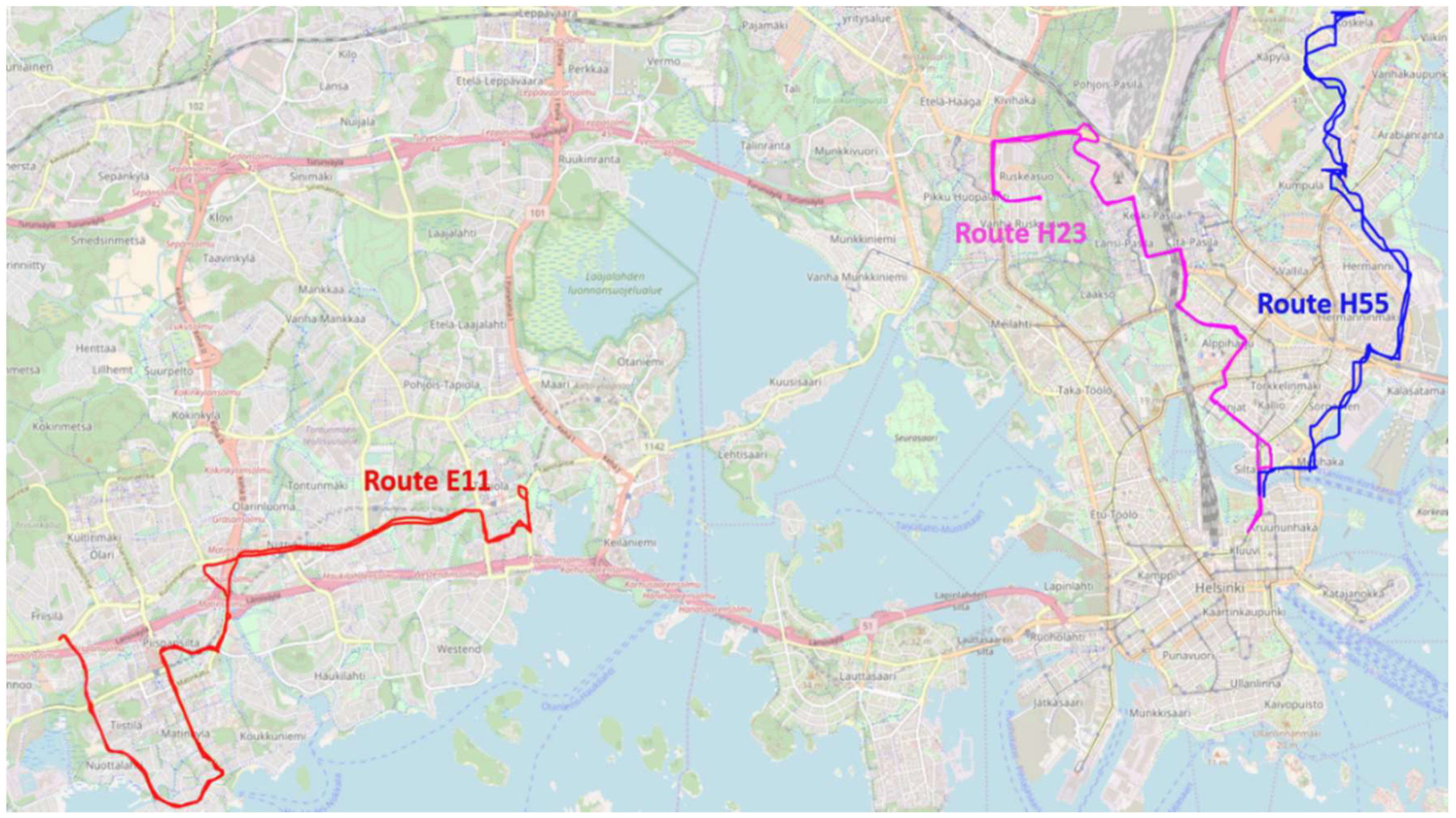
3.1. Buses and Routes

Six electric city buses were monitored during their normal daily operation over the years 2016–2017. The monitored buses (referred to individually here as E1, E2, H1, H2, T1, and T2) operated in the Finnish capital city, Helsinki, and the suburban city of Espoo. The buses E1 and E2 were BEB prototypes, but were comparable to a finished product. They were originally diesel buses that had their powertrains replaced with electric ones. The other four buses were designed based on these prototypes. All of the buses were designed as low-weight BEBs with an aluminum frame from Kabus Oy. The technical specifications of the buses are listed in Table 1. The electric heat pump was used for light heating and air conditioning. The heat pump was supported with a separate diesel heater, which adds up to 24 kW extra heating power during winter [28].
Buses E1 and E2 operated only on Espoo bus route 11 (E11), which is highlighted in red in Figure 1. Buses H1 and H2 were assigned to operate on Helsinki route 23 (H23). The last two buses, T1 and T2, operated first on route E11 and were later assigned to Helsinki route 55 (H55). Unfortunately, the GPS coordinate data of bus H2 were not as accurate as those of the other buses, so only the fast-charge events of this bus were analyzed. Furthermore, the GPS data of buses T1 and T2 were not as dependable as that of the rest of the buses, as can be seen from the inconsistency of route H55 in Figure 1. Nevertheless, there were enough data to parse different driving cycles and to analyze driving mission parameters because all the relevant signals (speed, power, current, voltage, auxiliary devices) had sufficiently accurate values during the operation.

3.2. Measurements

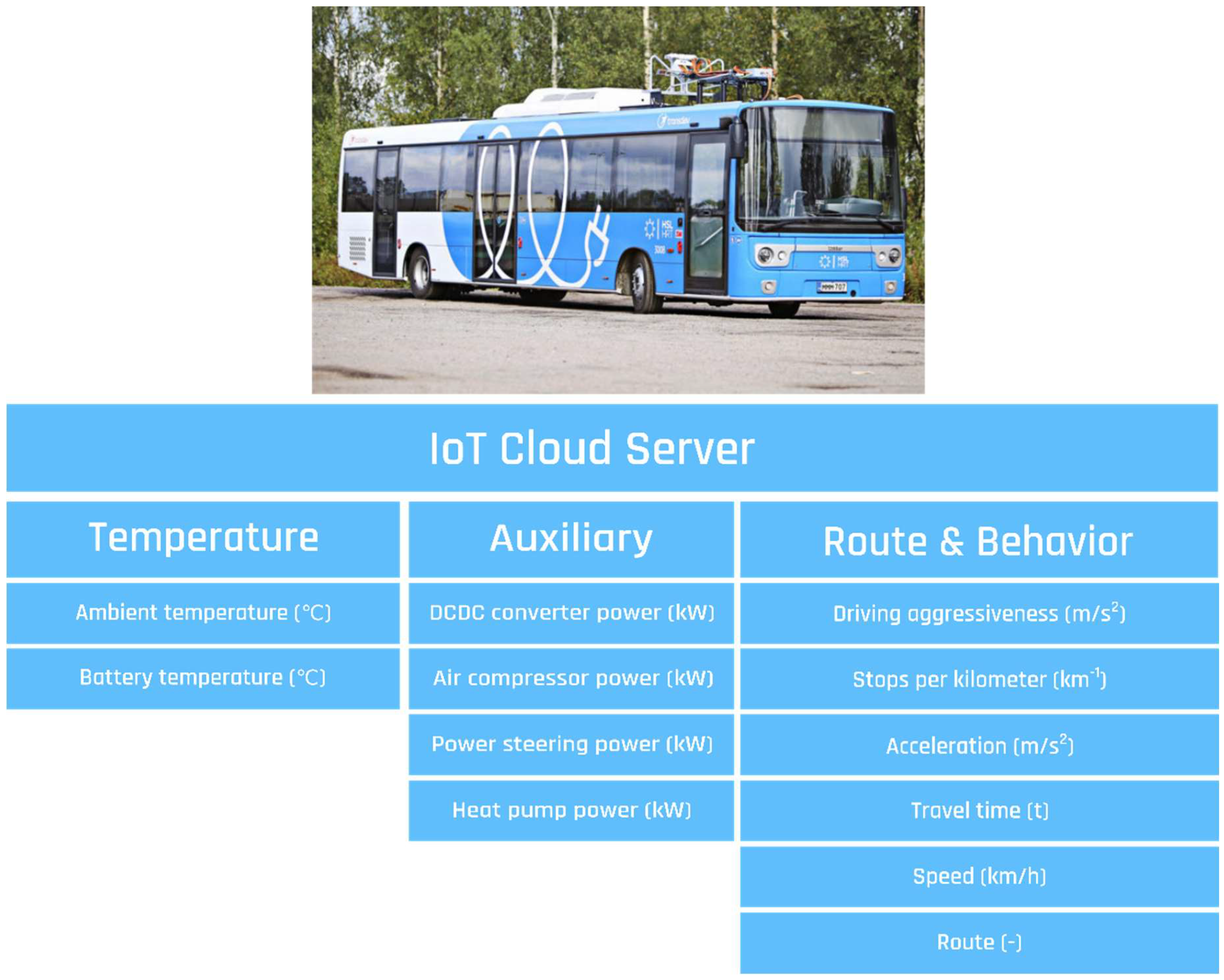
3.2.1. Data Collection

The objective of the data acquisition was to measure the relevant operation factors, which were either measured or computed from the measured signals. For practical reasons, the buses were measured as a part of an Internet of Things (IoT) system. The measured data of the bus were sent to an IoT cloud server for storing. The operation factors were divided into three categories: temperature, auxiliary, and route and behavior factors, as shown in Figure 2.
The sample time frequencies of the measured signal varied from 0.2 to 2 Hz. The sample time was not synced between signals because data were only recorded if the value of the signal changed, to minimize size of the stored data. Therefore, the signals were normalized to a common 10 Hz frequency with a linear interpolation fit. The normalization was especially essential for accurate positioning, as the GPS coordinates were not originally in sync. The normalization was also accompanied by a data point fixing algorithm that kept the last signal value measured until a change in the value was observed. Without data point fixing, the linear interpolation would misinterpret the measured data. To demonstrate the effect of signal normalization and data point fixing, an example of signal filtering is presented in Figure 3. At first glance, the raw signal seems to be logical because it is continuous, yet the battery current control used was discrete.
The ambient temperature was measured with a sensor attached to the chassis of the bus and the battery temperature was measured at each of the battery modules. A temperature sensor was placed on the surface of one cell per module and the average of those temperatures was considered as the temperature of the battery pack. The battery pack temperature was controlled with a liquid cooling system that prevented it from overheating during charging and discharging. However, the temperature still increased during charging and the longer the battery was charged with a constant power the hotter it became. Therefore, the cooling system was able to limit the temperature rise, but not eliminate it.
The battery state-of-charge (SOC) was measured continuously during bus travel and discharge, yet our interest was in its value at the beginning of each discharge and charge. Our hypothesis was that a depleted battery could cause higher consumption than a charged one, because some studies indicate higher battery resistance at lower SOC levels [30]. The current and voltage of the battery were measured from the battery management system (BMS) that tracks the battery’s state of health (SOH) and cuts the power in case of emergencies. BMS also calculates an SOC estimate based on the battery’s open circuit voltage characteristics.
Vehicle speed was measured from the motor encoder with the frequency of 1 Hz and the acceleration was computed from the speed profile. The acceleration estimate was determined to be accurate enough when compared with a previous study [11], where the same bus as the one studied here was simulated driving route E11. Furthermore, Shankar & Marco [24] noted that 1 Hz sampling rate is the minimum requirement for reliable consumption analysis. The powers of the auxiliary devices were measured from their respected controlling systems.

3.2.2. Discharge Cycles

The discharge and charge cycles were parsed from the raw data based on bus GPS coordinates. One discharge cycle, or a trip, was captured when the bus passed by two different terminuses in less than an hour. The focus on discharge analysis was on energy consumption and regenerative braking. The specific interest was on how the variation in operation factors shown in Figure 2 affected the energy consumption and regeneration variation. Therefore, energy consumption per distance d travelled, E d , was calculated with
E d = 0 t ( P b ( t ) )   d t 3.6 · 10 3 · d
where P b ( t ) is the electrical power signal of the battery pack as a function of time. In addition to energy consumption, we also calculated the driving aggressiveness on route. Driving aggressiveness is not a well-known factor, but it has been acknowledged before by Lajunen & Kalttonen [11]. They noted that as the aggressiveness on route increases, so does the energy consumption. For this reason, we have included it in our analysis, determined by
A g g = 0 t ( v ( t ) · a ( t ) )   d t 0 t v ( t )   d t
where v ( t ) is the time dependent speed of the bus and a ( t ) is the positive acceleration. The aggressiveness increases significantly if there are accelerations at high speeds, when the acceleration causes more energy consumption, which is why it is a better consumption predictor than the average acceleration.

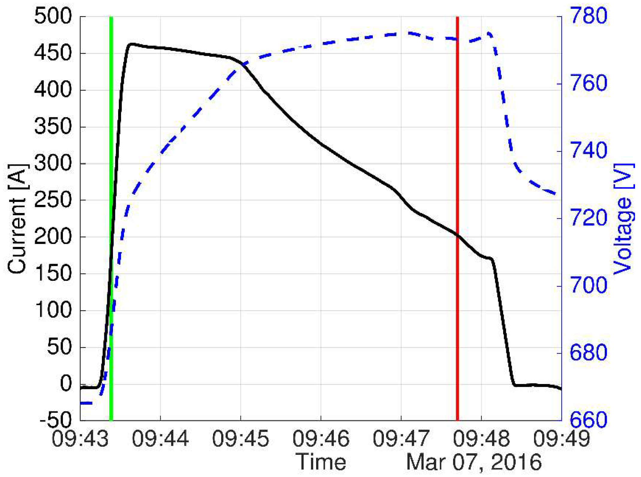
3.2.3. Charge Cycles

Only one of the two terminuses on each route had a charging station, so the charging occurred after every other trip. The charging events were extracted from the raw data using a charge current threshold of 200 A. The current threshold was chosen because most of the battery charging was done with currents higher than 200 A, as shown in the example charging event in Figure 4. The battery was charged with constant power of 340 kW when SOC was under 60%. After this threshold SOC, the power was reduced linearly until the end of the charge.
The quantity of interest during the charging events was on the internal resistance of the battery pack. The internal resistance was dependent on aging, current, SOC, depth of discharge (DOD), and temperature of the battery [31,32,33]. The impact of temperature on the internal resistance of lithium-ion batteries was roughly an order of magnitude greater than the impact of degradation [34]. Our hypothesis is that the variation in the internal resistance during charging is caused mainly by the temperature and charge current, yet the relative contributions of these factors to the internal resistance variation are unknown in real-world operation. The internal resistance of the battery pack can be estimated from the acquired charge cycles because the open-circuit voltage V o c v of the battery pack is known as a function of state-of-charge S O C ( t ) . This information is provided in the battery data sheet. At any given moment, the internal resistance I R B ( t ) is defined as
I R B ( t ) = V b ( t ) V o c v ( S O C ( t ) ) I b ( t )

3.3. Sensitivity Analysis with Multiple Linear Regression

3.3.1. Background

Most engineering systems have input values—some adjustable, and some noisy and unpredictable. The adjustable factors can have minor variation because of tolerances, but the unpredictable factors can have much more variation. The input factor variation propagates into variation in the system output and performance. Uncertainty quantification (UQ) is a method to show the variation in the system inputs and outputs, yet it does not describe the relations between these variations. Based on the UQ results, a global sensitivity analysis (GSA) can be carried out to gain a deeper understanding of the behavior of the system under varying conditions [35]. A GSA provides insights for design engineers and researchers to determine which unpredictable noise factors cause the most variation in the system performance. With this information, engineers can focus directly on reducing the effect of the input factors that are the most critical to the system performance.
Single output GSA methods, such as the method of elementary effects [35,36], the derivative-based method [35], principal component analysis (PCA) [37], the moment dependent method [35], and the variance-based method [35,38], are applicable to analyze the sensitivity of simulation models and measurements. Because, in many engineering applications, the goal is to reduce variation in the system performance, the variance-based method is the most straightforward approach to cases where analytical models are not available, as in our case. Sobol’s sensitivity indices can be calculated without a surrogate model, if there is experimental control, such as in Monte Carlo simulations. If there is no experimental control, a surrogate model is needed to represent data. However, most of the surrogate modelling methods are based on the hypothesis that the input variables are uncorrelated, which is unlikely in complex engineering challenges. However, sensitivity analysis with surrogate modelling of correlated input factors has received more attention recently.
Xu & Gertner [39] proposed partial variation decomposition, where the total sensitivity index is further decomposed into partial variation parts, which are the uncorrelated and correlated contributions. They considered only linear effects with a multiple linear regression (MLR), whereas Li et al. [40] proposed a state dependent regression (SDR) approach, which also considers nonlinear effects. Mara & Tarantola [41] approached the issue by decorrelation of the correlated input factors before analyzing them. Later, Chastaing & Camboa [42] proposed a generalized Hoeffding–Sobol decomposition for sensitivity analysis of correlated input factors.
We revisit the work of Xu & Gertner [39] and Li et al. [40] and combine their approaches by developing an MLR surrogate model, which is then analyzed with partial and second-order variance decomposition analysis. Decorrelation of input factors [41] or the use of generalized decomposition [42] is not as straightforward as the MLR variance decomposition approach. This is because of the multicollinearity issues of our case.

3.3.2. MLR with Correlated Inputs

An MLR of a function y = f ( x 1 , x 2 x i , x K ) , consisting of factors of interest x i , can be represented as
y = β 0 + i = 1 K β i x i + e
where β 0 β K are regression coefficients, K is the number of factors, and e is the error. With multiple observations N , the input factor space is presented as
X = [ x 11 x 1 K x N 1 x N K ]
and the MLR is described with a vector of compatible dimensions,
Y = ( y 1 y N ) = [ f ( x 11 x 1 i , x 1 K ) f ( x N 1 x N i , x N K ) ]
The variance of the linear regression model output V can be decomposed as
V = i = 1 K V i + V e
where V i is the output variance contributed by the factor x i and V e is the contribution of the factor uncorrelated error of Equation (4). The model variances are approximated with
V ^ i = β ^ i 2 v a r ( x i ) = 1 N 1 β ^ i 2 j = 1 N ( x j i x ¯ i ) 2
V ^ = v a r ( y ) = 1 N 1 j = 1 N ( y y ¯ ) 2
where V ^ i is the approximated variance caused by factor i and its interactions. V ^ is the approximated total output variance. With the factor matrix X and output vector Y , the least-square estimates of regression coefficients β can be solved with
β ^ = ( β ^ 0 β ^ i β ^ K ) = ( [ 1 _ N X ] [ 1 _ N X ] ) 1 [ 1 _ N X ] Y
where 1 _ N is a column vector of 1’s with the length N . With these estimated regression coefficients, the estimated output of each observation j in N can be calculated by
y ^ j = β ^ 0 + i = 1 K β ^ i x i
The observation correlated model outputs are used to acquire the total output variance of the model,
V ^ L = 1 N 1 j = 1 N ( y ^ j y ¯ ) 2
where V ^ L is the total variance of the approximated model and y ¯ is the mean output. Comparing the measured output variance and the approximated one, the R 2 value of the model fit can be computed as
R 2 = V ^ L V ^
The R 2 value lies between 0 and 1. The R 2 (R-squared) value is a statistical coefficient that is used to define the goodness-of-fit of surrogate models.
Once the approximated model is sufficiently accurate, the variance caused by the input factors can be further divided into contributions of each of the variables and their interactions with a high dimensional model representation (HDMR). HDMR is a decomposition of function hierarchy, such that portrays a function as a sum of factor-specific sub-functions. Truncated HDMR combined with analysis of variance (ANOVA) variance decomposition [39,43,44,45,46] results in
V = i = 1 K V i + i < j V i j + + V 1 K
However, the ANOVA decomposition does not hold if the input parameters are correlated. However, even if the input parameters are correlated, the output variation can be further decomposed into partial variation contribution, as proposed by Xu & Gertner [39]. The partial variance contribution of one factor has a linear, uncorrelated effect on the output variance and a correlated component that is caused by the interactions with other input factors. Thus, the factor variation contribution V ^ i can be split into uncorrelated V ^ i U and correlated variation contribution V ^ i C , such that
V ^ i = V ^ i U + V ^ i C
To calculate the uncorrelated component, we use the expression
V ^ i U = 1 N 1 j = 1 N ( y ^ j ( i ) y ¯ ) 2
where
y ^ j ( i ) = r ^ 0 + r ^ i z j i
The regression coefficients r ^ 0 and r ^ i can be solved with
( r ^ 0 r ^ i ) = ( [ 1 _ N Z ^ i ] [ 1 _ N Z ^ i ] ) 1 [ 1 _ N X ] Y
where the residual regression matrix is
Z ^ i = ( z ^ 1 i z ^ N i ) = [ x 1 i ( η ^ 0 j s 1 K η ^ j s x 1 j s ) x N i ( η ^ 0 j s 1 K η ^ j s x N j s ) ]
The residual regression matrix regression coefficients are described as
η ^ = ( η ^ 0 η ^ j s η ^ K 1 ) = ( [ 1 _ N X ( i ) ] [ 1 _ N X ( i ) ] ) 1 [ 1 _ N X ( i ) ] X ( i )
where X ( i ) is a factor matrix excluding the factor x i and X ( i ) is a vector of only the factor x i ’s observations. The variation among the residuals z ^ j i is uncorrelated with all the other factors x j s ( j s 1 ) , because of its perpendicularity to η ^ , and so the variation explained by y ^ j ( i ) is solely contributed by the factor x i . After solving Equation (16), the correlated partial variance can now be determined with Equation (15). The relative measure of the variance components to the total variance is presented with Sobol’s sensitivity indices [44]. The sensitivity index ( S i ) of a factor x i can be divided into uncorrelated and correlated sensitivity indices ( S i U and S i C ), calculated as
S i = V ^ i V ^
S i U = V ^ i U V ^
S i C = V ^ i C V ^
In addition to the MLR variance decomposition approach with partial variance decomposition proposed by Xu & Gertner [39], other methods that consider correlated inputs have been developed. Li et al. [40] proposed a state dependent parameter approach, which considers nonlinearities, unlike the MLR. They also introduced an importance matrix, which represents second-order interactions between factors. The sensitivity indices of second-order interactions are governed with
S l , q C = V ^ l , q C V ^
An importance matrix displays the relation between factors, which takes the form
S = [ S 1 U S 1 , N C S N , 1 C S N U ]
where the diagonal consists of the uncorrelated sensitivity indices and all of the other sensitivity indices are factor–factor interactions. The upper and lower triangles are symmetrical in relation to the diagonal because the interactions’ effect is equal in both directions ( S N , 1 C = S 1 , N C ). The sum of the diagonal and the upper triangle should always be less than or equal to unity, because the decomposed output variance in Equation (14) is divided among the factor contributions, hence
1 i = 1 K S i + 1 i < j K S i j + + S 12 K
holds when the input factors are uncorrelated.

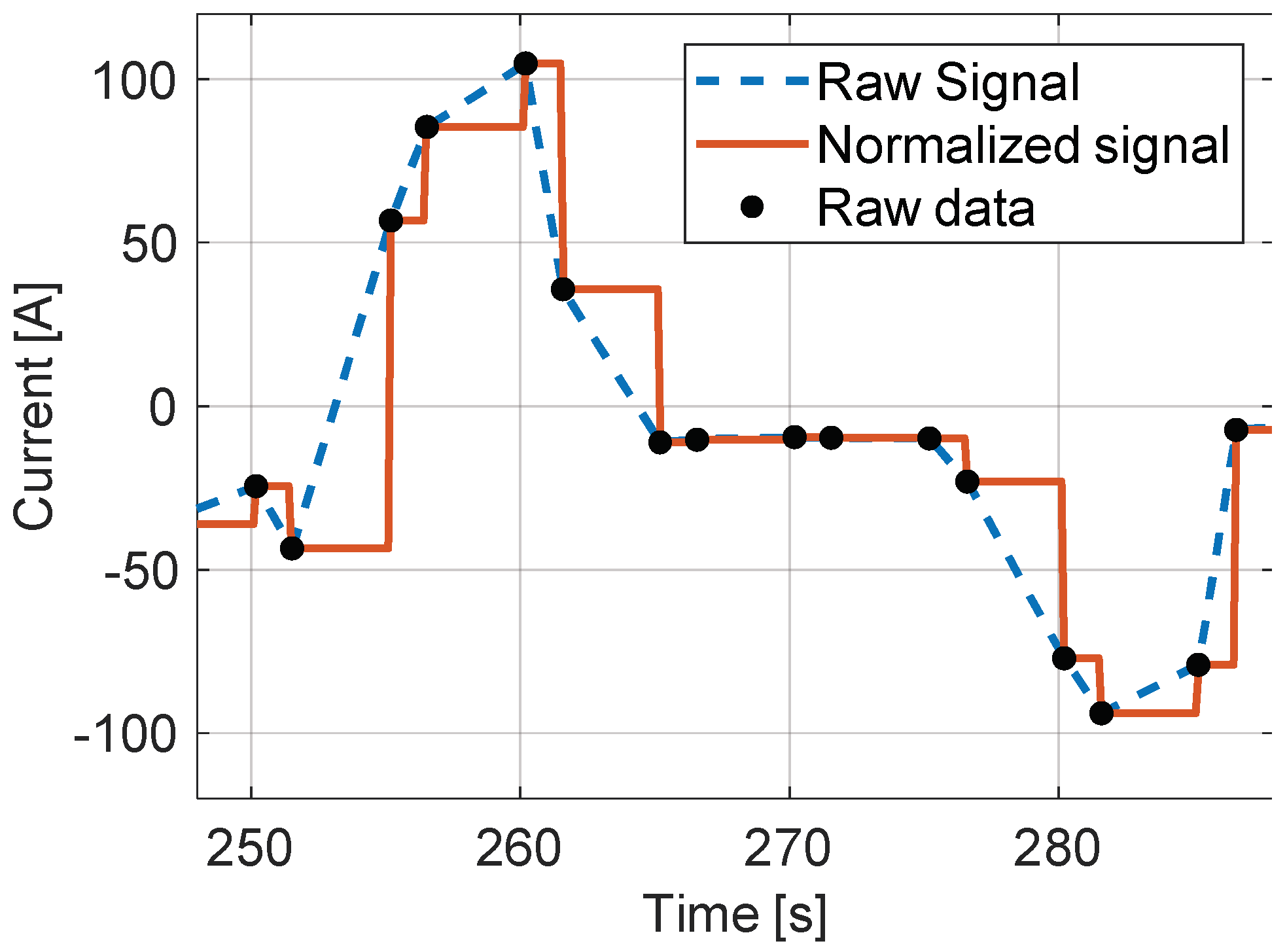
3.3.3. Normalization of Second-Order Effects

In order to adequately understand the second-order effects of correlated factors, the importance matrix needs to be normalized. Without normalization, the sum of second-order effects is larger than the correlated contribution of an input factor and becomes difficult to comprehend. Therefore, a normalization approach is proposed to improve the comprehension of second-order interactions when the factors are correlated. However, the normalization gives legitimate results if the higher than second-order effects are minor.
The normalization process is implemented as follows. First, the diagonal effects are nullified, because they are not considered in the sum of second-order effects,
[ S 1 U S 1 , N C S N , 1 C S N U ] [ S 1 U 0 0 S N U ] = [ 0 S 1 , N C S N , 1 C 0 ]
Next, each column of the importance matrix S is divided by the sum of the column elements, which is computed as
[ 0 S 1 , N C S N , 1 C 0 ] [ i S i , 1 C 0 0 i S 1 , i C ] 1 = [ 0 S 1 , N R C S N , 1 R C 0 ]
where the superscript R C refers to the relative correlation part. Finally, each element of the column is multiplied by the correlated sensitivity index of the factor X i . This is done to achieve normalized effects in respect to the second-order sensitivity index rather than unity. The normalized importance matrix S N 2 is represented as
S N 2 = [ 0 S 1 , N R C S N , 1 R C 0 ] [ S 1 C 0 0 S N C ] = [ 0 S 1 , N N C S N , 1 N C 0 ]
where the superscript N C refers to the normalized correlation part.

3.4. Statistical Analysis

Correlation between two factors is the measurement of how similarly they behave. A Pearson correlation coefficient is the most common metric for linear correlation and its values lie between −1 and 1. Here, we refer to the Pearson correlation as correlation. If the correlation between two factors is 0, then they are linearly independent and uncorrelated. If the relationship between two variables is linear, the correlation is equal to the Sobol’s total sensitivity index.
High correlation between two factors is also referred to as collinearity. In the case of multicollinearity, multiple correlations occurs among many of the factors, and hence the correlations are global. Severe multicollinearity can cause erroneous predictions in multivariate linear regression [46]. Multicollinearity can increase coefficient of determination, yet single factors can remain statistically insignificant. Multicollinearity can also reverse the regression weight directions. There exists many ways to detect multicollinearity and one popular method is to measure variation inflation factor (VIF) [46].
VIF is calculated by fitting a multiple linear regression to predict one of the input factors using the rest of the input factors as predictors. If the resulting VIF factor is 10 or higher, multicollinearity is severe. However, some statisticians state that factors that have VIF higher than 5 should be left out of the analysis [46,47]. The squared root of VIF is the multiplier effect of how much larger the standard error in a model is compared with the situation where the factors are uncorrelated. One way to perform linear regression even when the factors are multicollinear is to perform stepwise regression.
The main approaches of stepwise regression are forward selection, backward elimination, and bidirectional elimination. Forward selection is the simplest, where factors are added to the model automatically until adding any factor does not make the coefficient of determination significantly higher. Here, we added the factors one-by-one based on which was the best to add and stopped when the improvement to the R-squared value when adding a factor was less than 2%. More sophisticated methods exists, yet with a small set of factors, simpler methods can be utilized [48]. In the process of stepwise regression, factors are left out, which increases the residual of the MLR. However, the change should not be significant, otherwise too many factors could be removed.
If the residual, or the error term in Equation (4), in the MLR model resembles a normal distribution, this means that it can be considered as unknown noise. This implies that the model is not overfitted. One advantage of using linear models is that overfitting is usually not an issue because the squared loss function aims to set the model in the center of the data. Another reliability factor is the p-value. The p-value of a factor is used to determine if a predictor in an MLR model has a meaningful impact to the output variable. The p-value is also used to discard factors that only seem to increase the R-squared value of the model, yet do not significantly impact the output variable.

4. Results

4.1. Operation Factors

A total of 14,058 discharge cycles and 13,549 charge cycles were measured from six operating battery electric city buses. After filtering and rejecting unusable measurements, 9418 discharge cycles and 5764 charges cycles remained for further analysis. Two of the buses (E1, E2) operated only in Espoo, which is a suburban area, and two (H1, H2) only in the Finnish capital, Helsinki. The remaining two buses (T1, T2) operated in both areas. During operation, 12 relevant operation factors were measured and 5 were computed afterwards. These factors are listed in Table 2. The data type of each factor is classified as total, mean, start, or single types. Total indicates the sum, mean indicates the average, start indicates the starting value, and single indicates one value during a discharge or charge cycle.
First, the correlations between operation factors were studied. The Pearson coefficient was applied to represent the approximate effect between factors. The analysis focused on determining which factors were the main contributors to the variation in the ECR, energy regeneration, and internal resistance of the battery. Furthermore, the objective was to identify linear and nonlinear relations.

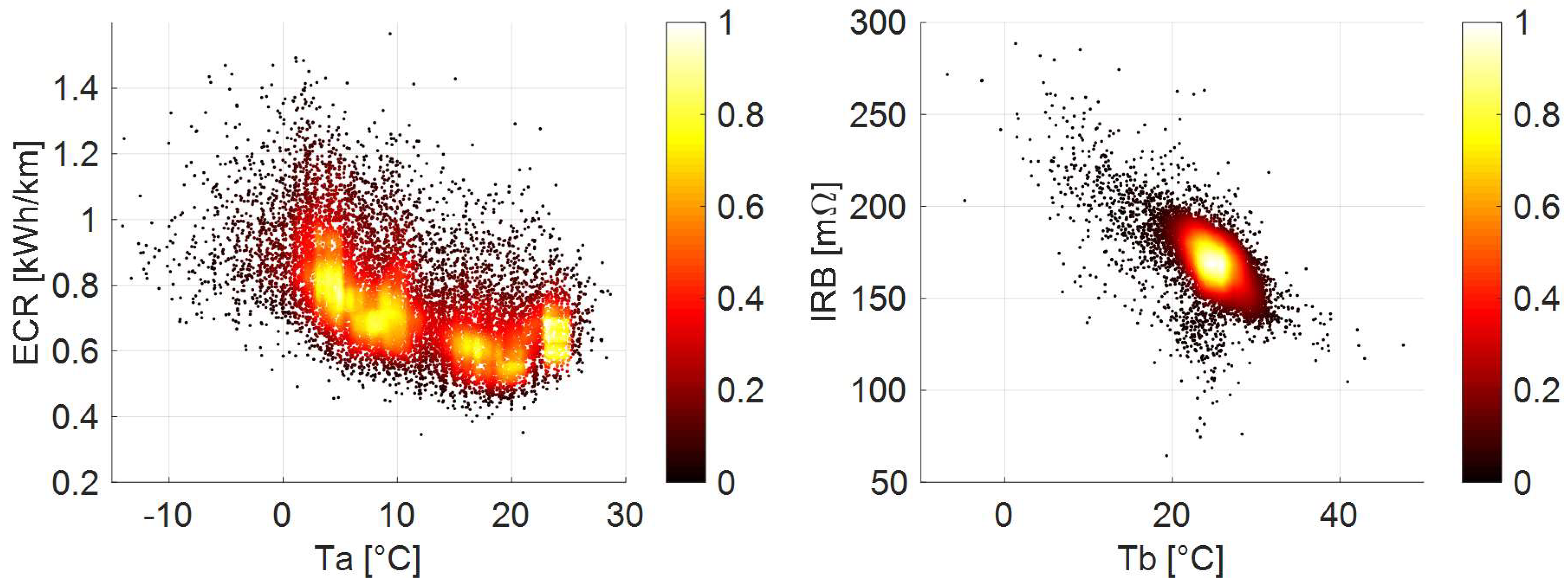
4.1.1. Temperature Factors

The temperature factors considered here were the battery temperature and the ambient temperature. The ambient temperature had a higher correlation with the ECR during discharges, −0.54, whereas battery temperature had a correlation factor of −0.19 with the ECR. During charges, the battery temperature did, however, correlate strongly with the IRB (−0.65), as shown in Figure 5, and the ambient temperature also had an impact (−0.34). The correlation between battery and ambient temperature during discharges and charges was 0.32 and 0.24, respectively. However, these correlations only consider linear effects. As shown in Figure 5, the ambient temperature has a parabolic relation with ECR, with the lowest value around 20 degrees Celsius, as is typical with electric vehicles and buses [14,49]. Therefore, we linearized the effect of ambient temperature around 20 degrees Celsius, | 20 T a | , which means that at that point, the effect of ambient temperature was negligible. The assumption was also made by De Cauwer et al. [25] in their research on the estimation of electric vehicle consumption. With this consideration, the correlation between ambient temperature and ECR is 0.58.

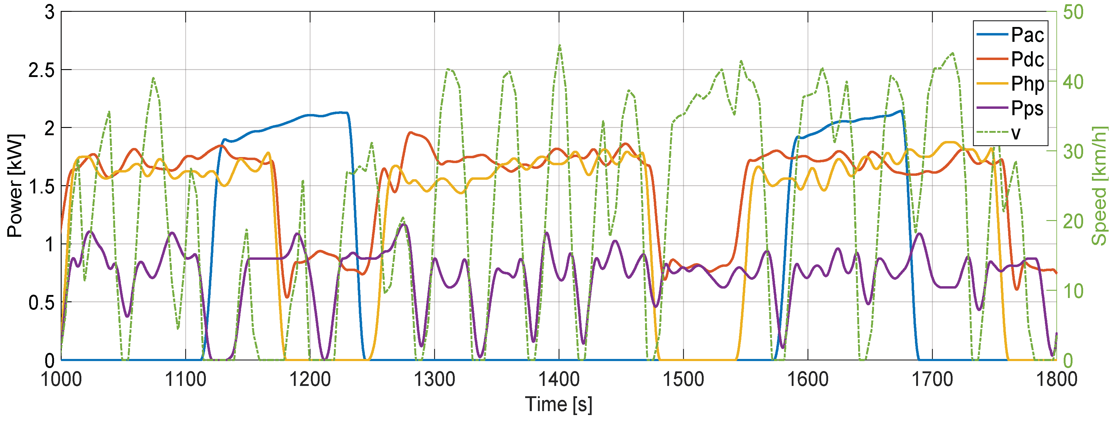
4.1.2. Auxiliary Devices

The auxiliary power of the air compressor (Pac), DC devices (Pdc), heat pump (Php), and power steering (Pps) was analyzed for discharge cycles. They were mainly turned off during charging. As seen from Figure 6, the total auxiliary power consists of DC device power and the air compressor power, because the air compressor is not part of the 24 V DC circuit. The air compressor is used to refill the pneumatic accumulator after door opening at a stop where a passenger has been picked up or dropped off. The DC device power was approximately the sum of the heat pump power and power steering power. The Pdc had a significant correlation with the ECR (0.68), as shown in Figure 7. Furthermore, the Pdc correlated most with the heat pump power (0.51), which is the reason for the high correlation (0.54) between the Pdc on Ta. The heat pump power depended on the ambient temperature and their correlation was 0.5. This indicates that the heat pump power setting is also affected by manual adjustments made by the driver and how many times the doors are opened, which is when heat energy is lost.

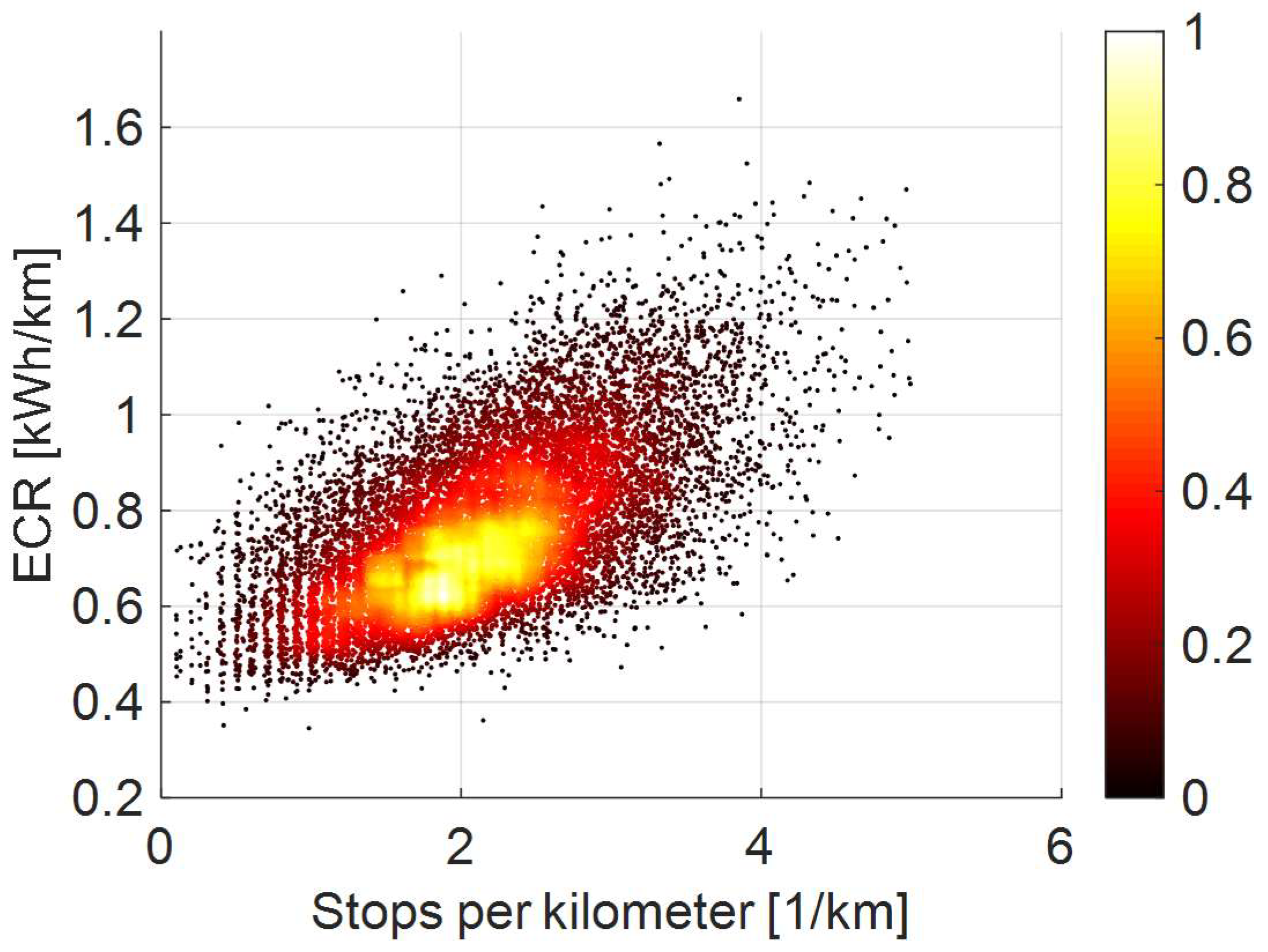
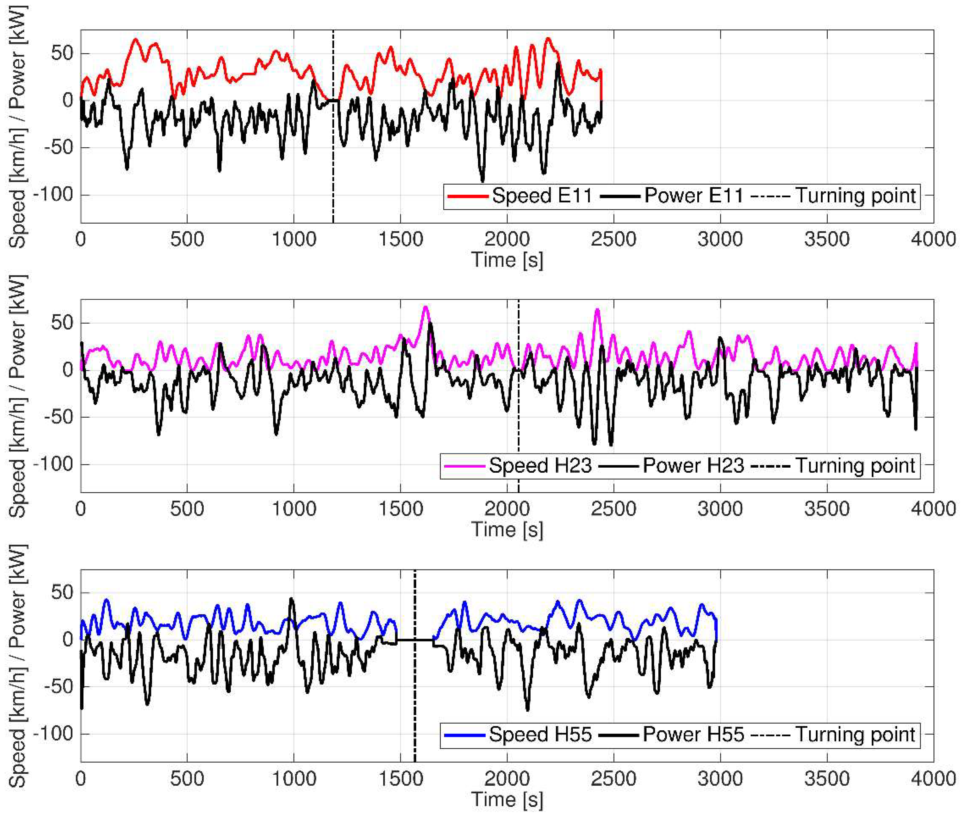
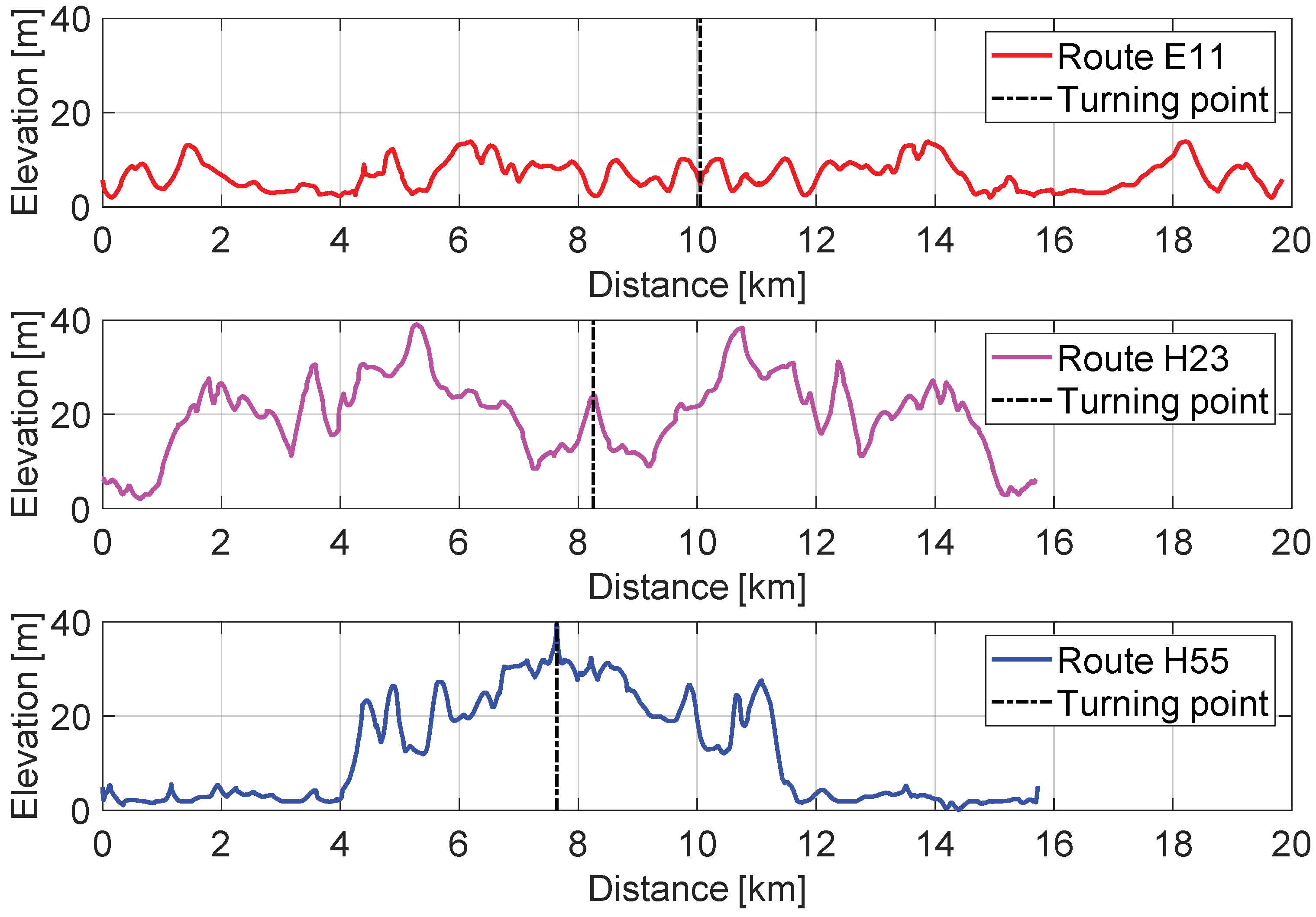
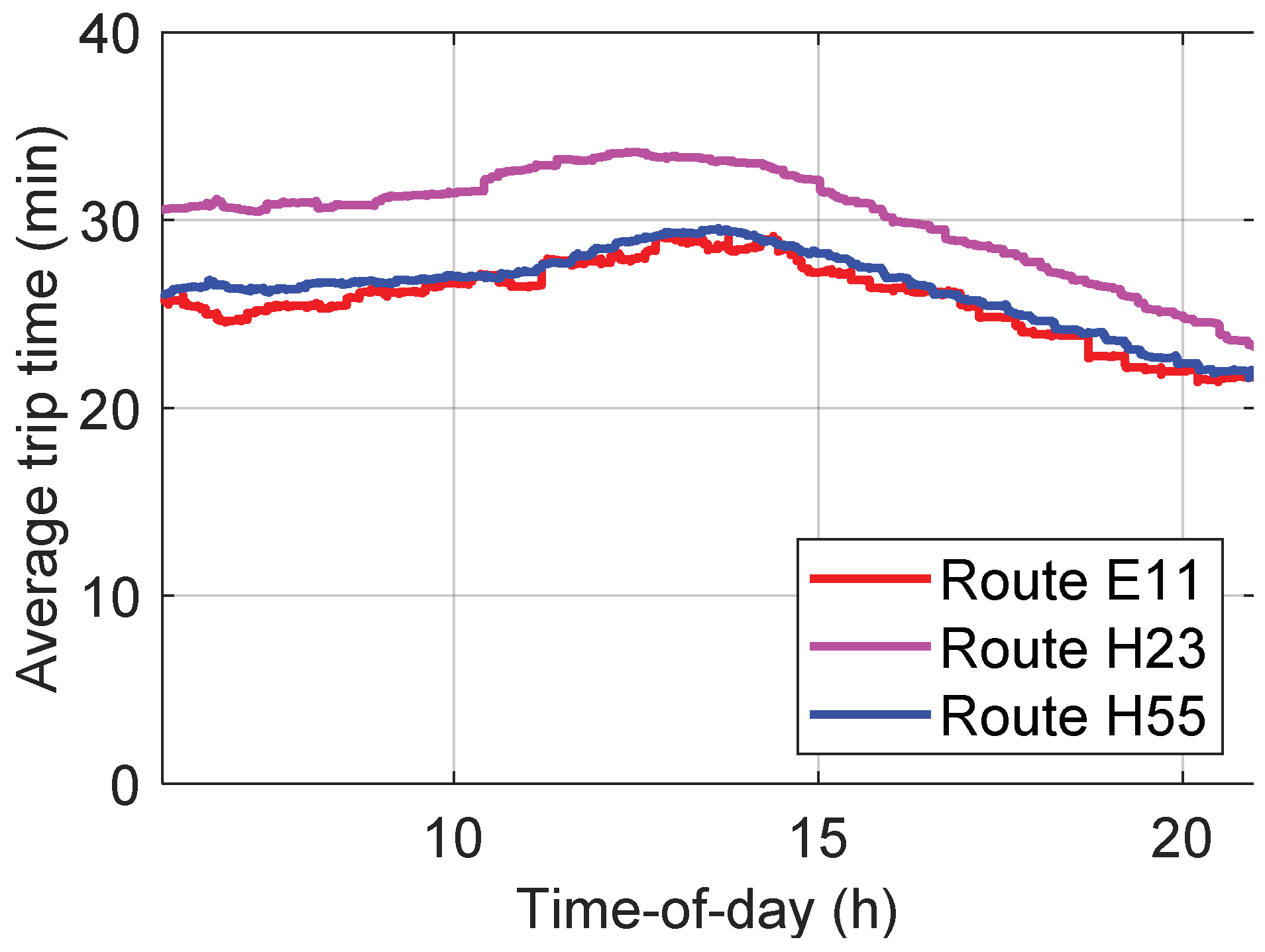
4.1.3. Route and Behavior Factors

The route and behavior factors were analyzed together because the route factors are strongly linked to the driving behavior and vice versa. Typical route and behavior characteristics include speed and acceleration factors such as average speed and average acceleration. Although information is lost because the aerodynamic drag and acceleration forces are not computed, the average speed is a common characteristic of a route. Furthermore, while designing a BEB, traffic conditions are challenging to simulate, so it is easier to estimate the distribution of average speed as a nominal distribution than as separate cycles that are needed for a more specific uncertainty quantification. Hence, here we used the average speed as a predictor, which, according to De Cauwer et al. [25], is an accurate consumption prediction for EVs.
Furthermore, the effect of acceleration can also be portrayed with driving aggressiveness. The linear correlation between the driving aggressiveness and the ECR was 0.49, as shown in Figure 8. The aggressiveness is more dominating with lower values (less variance) and with higher values, the effect is more scattered. The dominance could be explained by the fact that at higher average speeds, there are less stops, and the aggressiveness is lower, yet accounts for more of the ECR than other route and behavior factors.
Driving aggressiveness does not consider the effect of idle time or stops per kilometer. However, idle time and stops per kilometer have a strong relation (0.8), and thus only one of them should be chosen as a predictor of ECR. The stops per kilometer was a better candidate, because even though it had the same correlation with ECR as idle time (0.6), the Spk had a more consistent relation with ECR, as shown in Figure 9.
Driving behavior is the combination of the driving style, route, and traffic effects. Three different routes were considered, with one of them operated in Espoo (E11) and two in Helsinki (H23 and H55). The speed and power profiles of these routes are shown as round-trips and a striped line indicates the turning point in Figure 10. The average speed is higher in the suburban city of Espoo and there are more frequent speed transients on Helsinki routes. Based solely on the speed profiles, the direction of the route evidently has a minor effect on the driving behavior. Furthermore, it is interesting that on some smaller decelerations, a lot of energy is regenerated through regenerative breaking on route H55. This indicates that the bus had already achieved a steady speed and was decelerating on a downhill.
In a similar fashion, the elevation profiles of the bus round-trips are shown in Figure 11. Espoo E11 route is significantly flatter than the other two routes, H23 and H55. Route E11 also ends and begins at approximately the same elevation level. Even though route H23 has a lot more variation in the elevation and even though the end of the trip is not on the same level as at the start, the consumption did not vary significantly on different route directions, although it did more than on route E11. The elevation profile on route H55 clearly affected the consumption depending on the route direction. While travelling towards the turning point, the elevation increased by almost 40 m with not much elevation variation. For this reason, the direction of route H55 had a correlation of 0.46 with ECR.
It is difficult to include the effect of elevation in real-world measurements in the consumption prediction. One approach is to divide a driving cycle into subcycles based on the elevation profile, where each of the subcycles has their own regression model. The sum of these subcycle models is the consumption prediction in the entire route. Even though this approach could result in more accurate predictions, in practice, this approach might only highlight measurement and modeling errors and not the effect of elevation [25]. These effects would be amplified in our case because the GPS coordinate data was synced as a part of the postprocess.
The last route and behavior related operation factor was traffic. Traffic affects many factors such as the number of stops, driving aggressiveness, and air compressor power, just to name a few. However, the influence of traffic is difficult to measure in real-time. Ritari [50] measured the traffic in Espoo using Google Maps traffic density information. Vehicle traffic was shown to be higher in morning traffic from 07:00 to 09:00 and from 15:00 to 18:00 in the afternoon. The trip time of buses did not correlate with the traffic density, as can be seen in Figure 12, where the longest trip times were in the period from 11:00 to 15:00. The increase in average trip time is probably the result of general business hours, when most of the stores are open and services are available. The difference between bus trip times on weekend and weekdays was marginal and most measured trips (93%) were driven on weekdays.

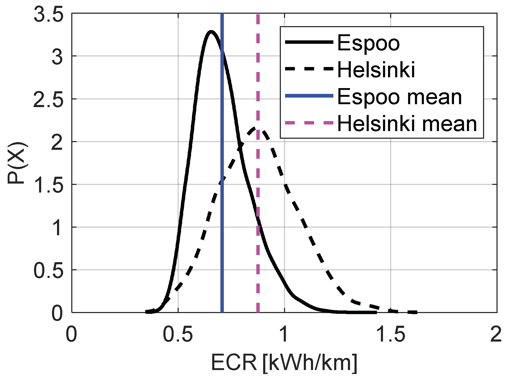
4.2. Energy Consumption Rate (ECR) on Discharges

42.1. Output Analysis

In order to inspect the ECR distribution, probability density functions (PDFs) for buses operating in both Espoo and Helsinki are shown in Figure 13. ECR was 24% larger on the Helsinki city route than on the Espoo suburban route. In addition, the Espoo PDF is skewed towards lower consumption rates, whereas the Helsinki PDF resembles more of a normal distribution. The skewing shows that it is more probable to have low consumption during operation on suburban routes. However, both PDFs share approximately the same minimum value. The higher dispersion of the ECR in Helsinki was partly caused by the direction correlation of the ECR on route H55. To compare the relative variation, coefficient of variation ( c v = σ / µ ) was applied as a standardized measurement of dispersion. The coefficients of variation were 0.18 and 0.19 for Espoo and Helsinki cycles, respectively.
As suburban routes have less traffic, the skew could be caused because of more favorable braking conditions. More energy could be regenerated with regenerative braking with controlled braking events than with sudden ones. However, the energy regenerated on the Espoo route was only 2% more on average compared with the Helsinki routes, as seen in Figure 14. The energy regeneration percent is the relation between all the energy consumed during a trip and the sum of energy regeneration with regenerative braking.
As the difference in the ECR between Espoo and Helsinki was not explained by regenerative braking, the operation factors were compared. The operation factors were chosen based on the operation factor analysis. In Table 3, the relative means and standard deviations on Espoo and Helsinki trips are presented. All of the operation factors were higher on Helsinki trips, except temperature. Thus, all of the operation factors were in a setting that increased the ECR. The decreased ambient temperature caused higher Pdc consumption. The ambient temperature should be constant when comparing route differences. However, increased stops per kilometer also increase Pdc, because it is consumed even when the bus is not moving. The increase in stops also increased driving aggressiveness and air compressor power. Considering these facts, it is safe to say that the difference between the Helsinki and Espoo average ECR is nevertheless at least 15%.
As an additional experiment, the acceleration limit of one of the Espoo buses, E2, was lowered from 2.1 m/s2 to 0.7 m/s2. The reason for this setting was an earlier study of the same bus on the same route, where the driving behavior of BEBs was compared with diesel buses [51]. The BEBs were driven 10% faster and accelerated 10% faster than the diesel buses. The lowering of the acceleration limit had an opposite effect to what was expected. The average speed was increased by 4% and the average driving aggressiveness by 14%. Thus, it would seem that limiting the driver’s ability to accelerate could lead to unwanted frustration and actually increase recklessness rather than reduce it. However, the acceleration limit change did not have a notable effect on the ECR.

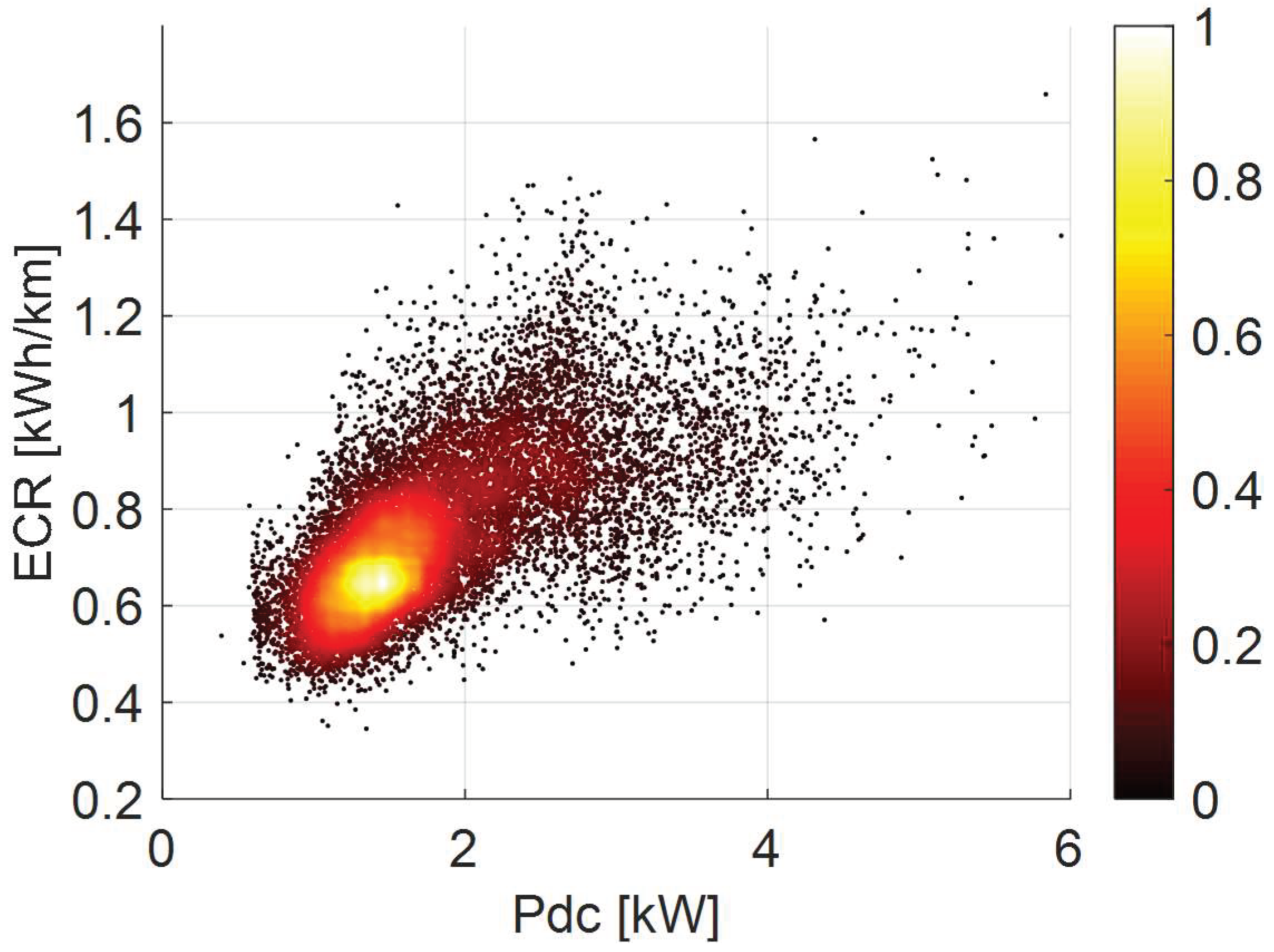
4.2.2. Input Analysis

The first thing to do while choosing input factors as predictors of ECR is to ensure that they have a linear relation. The direction of the cycle had a nonlinear effect because the studied routes had varying elevations profiles, as seen from Figure 11. The effect of ambient temperature (Ta) was taken as an absolute value with respect to 20 degrees Celsius, because its effect on ECR is parabolic around this value.
Next, a check for collinearities and multicollinearities was done with defining VIF values of the input factors. As seen in Table 4, Idle, Spk, and v are over the threshold of VIF = 5, which indicates multicollinearity. Therefore, some or all these factors should be left out of the linear model to avoid large standard errors. Stepwise regression with forward selection was used to select which factors were included in the final model.
In forward selection, one factor is added to the model at a time based on which factors improves the coefficient of determination the most, until a termination criterion is met. The chosen termination criterion was minimum model improvement of 2%. In Figure 15, the forward selection process is shown, and visible saturation is seen in the coefficient of determination after termination criterion was reached. The factor Ta was still included in the model, which improved the R-squared value by 6%. VIF values of the selected factors were rechecked and were all lower than 1.5.
The resulting linear regression model for ECR (kWh/km) based on all measured trips was
ECR ^ = 0.15 + 0.006 | 20 T a | + 0.1 P d c + 0.07 S p k + 1.25 A g g + ε
with R 2 = 0.76 . The R 2 value was 0.81 when all factors were included in the model, so the statistical power lost when dropping factors was insignificant. Furthermore, Saltelli [38] suggested a general rule of thumb that models with R-squared values significantly less than 0.7 might not be accurate enough and would need more data, or the modelling technique should be reconsidered. To validate the linear model fit, the distribution of the residual term ε is shown in Figure 16. The error term is roughly normally distributed, although slightly skewed towards negative values, resulting in consumption predictions slightly smaller than anticipated. Furthermore, the error term distribution shows that the linear model is sufficient and reliable. In addition, the p-values of the meaningful factors were less than 0.0001.
A sensitivity analysis of the meaningful factors is shown in Figure 17a. The Pdc had the highest uncorrelated effect on consumption and was heavily correlated with ambient temperature. Thus, because heat pump power was also a strong influencer of the Pdc, it could be deduced that environmental conditions that are temperature dependent cause most of the variation in the ECR. However, a close second contributor was stops per kilometer. The stops on route cause increased use of pneumatic doors, and thus higher Pac and higher driving aggressiveness (Agg) due to an increased number of accelerations. In summation, the sensitivity analysis showed that most of the crucial operation factors are highly correlated. However, the heating and environmental factors are almost independent of the behavior factors, because they consume energy and cause losses even when the BEB is at standstill.
The partial variance decomposition in Figure 17b confirms these deductions. The normalization of these effects enables the use of them in a case where there are correlations. From these second-order effects, it is seen that the environmental factors Pdc and Ta correlate mainly with each other and the route factors Spk and Agg with each other. Therefore, these factors can be multiplied to quantify the effect of these factor groups, which is also referred as compounds. As there is a slight correlation between the groups, the R-squared value reduced to 0.73 when the factors were grouped. In Figure 18, the variance decomposition of ECR is shown. The environment effects are slightly more dominating of the ECR variation. There was also a correlated effect with the route factor group, yet it was minor. The residual effect includes measurement errors and the effect of factors that were not included in this study, such as headwind, payload, mechanical braking and unknown factors.

4.3. Internal Resistance of the Battery (IRB) on Charges

4.3.1. Output Analysis

Low temperature and high current have been previously shown to increase battery resistance [32]. However, the range of internal resistance variation is of interest when planning charging schedules under uncertainty, because the IRB is proportional to required charging power and time. The nominal resistance of the bus battery pack was 75 mΩ and approximately 90 mΩ with the conductors. The average resistance during charging was 170 mΩ. The battery charging efficiency was distributed almost normally around the nominal value of 92.1%. The standard deviation was 0.7%. The variation of the battery recharge efficiency was not significant when compared with the variation in ECR.
For example, let us consider a scenario where the charging power is limited to 400 kW and so charging of a 20 kWh battery would take 3 min. A 2% decrease in charging efficiency would increase the charging time by 3.6 s. However, if the consumption doubles on route, from 0.5 kWh/km to 1 kWh/km, twice as much charging is required and so the charging time would also double. Thus, the charging efficiency fluctuation can be neglected while planning charging schedules because the ECR variation is much more significant. However, permanent resistance growth caused by aging and wear of the battery must be considered in scheduling and is also an important issue from maintenance and longevity perspectives.
The calendar aging is expedited by charge–discharge cycles, excessive charges, unfavorable depth-of-discharge, and elevated temperatures [52,53]. Even though the lithium titanate oxide (LTO) batteries have a long life expectancy, the resistance growth over time was analyzed because it affects the sensitivity analysis of the IRB. The charging events were fitted with a fourth-degree polynomial for each of the buses to represent resistance during charging as the charging cycles increase, which is displayed in Figure 19. The H1, H2, Tr1 and Tr2 buses exhibit only minor resistance variation compared with the sinusoidal variation of the E1 and E2 buses. The E1 and E2 were prototype buses and the peak resistances were at the coldest days in winter time and lowest during the summer. This implies that the insulation of the batteries is worse than in the newer buses. Thus, the internal resistance of the battery pack had no notable growth due to aging with less than 2500 cycles. Typically, LTO batteries can endure over 10,000 cycles before the resistance has grown 20% [2], which indicates end-of-life for a battery in vehicle use [18].

4.3.2. Input Analysis

The input factor analysis was carried out in a similar manner as for ECR. Charging time and SOC had unclear effect, if any, on the IRB and were thus left out of the analysis. Multicollinearity was not an issue, yet the effect of ambient temperature was so minor that it was left out of the model. The linear approximation model for the IRB (mΩ) based on measured charging events is
IRB ^ = 168 2.4 T b 0.2 I b + 0.2 V b
with R 2 = 0.58 . The R-squared value is significantly lower than the threshold of 0.7, so it is clear that these factors do not explain the entire variation of the IRB. However, because the variation of the IRB was minor, there was probably more noise in the measurements than in the case of ECR. In addition, the IRB model was limited to the battery operating range and extrapolated inputs were not considered here. The direction of the battery current term was unexpected. High currents led to lower IRB values. This was because the average current was lower when charging at high SOC levels as the battery charging power is linearly decreased after reaching 60%. This resulted in an increase in battery temperature, which lowered the resistance and explained the correlation between the two as seen in the sensitivity indices of Figure 20a,b. The uncorrelated effect of battery temperature was three times higher than that of battery current. In addition, the effect of battery voltage was low, yet it increased the statistical power of the model. The p-values of all the factors were less than 0.0001. Further analysis of the model reliability is not of interest because the coefficient of determination was low. Thus, the model was not intended for IRB prediction, but it was essential for the sensitivity analysis.

5. Discussion

The ECR of electric city buses varies significantly. The analysis shows that the variation is dependent on the environmental conditions, route, and driving behavior. However, there are other factors, such as rolling resistance, payload, and headwind, that were not measured here, yet play a role in the consumption variation. The payload is related to stops on route because the bus stops to pick up passengers. Furthermore, even though the ambient temperature affects charging scheduling, the average increase of the ECR is only 10% over a year of operation because of changes in season [14]. Therefore, the recharging schedules of BEBs could be designed with the season in mind for better predictability.
The operation factors were multicollinear, which caused challenges in the statistical and sensitivity analyses. For example, the idle time spent on route correlated with the number of stops on route, yet they are distinct characteristics. The strong correlation is probably the result of the fact that the stop times are fairly regular for buses, but the variation in the idle time of passenger cars can be more unpredictable. There is a substantial amount of dedicated bus lanes in the Helsinki metropolitan area that also alleviate public transportation flow in times of heavy traffic.
Sensitivity analyses of ECR and IRB were carried out with the use of MLRs. The MLR R-squared values were 0.76 and 0.58 for ECR and IRB, respectively. The residual indicates that there were some factors left unconsidered. Pihlatie et al. [1] noted that 6% and 12% of the BEB consumption is caused by aerodynamic drag and the use of mechanical brakes, respectively. In our previous study, we found that up to 18% of the ECR variation of BEBs is caused by rolling resistance variation and 13% by payload variation. To acquire even more accurate results, the effect of the minor exponential behavior of ambient temperature could have been described using a surrogate modeling technique that considers nonlinear behaviors. For nonlinear data-driven models, the SDR approach presented by Li et al. [40] offers many possibilities.
Including more of the operation factors in the MLR also increased the R-squared value, even close to 0.9 for both the ECR and IRB models when nonlinear effects were considered. However, it is a typical pitfall in statistics to use predictors that do not have a causal relationship to the output, but are considered just to improve the model accuracy. The operation factors chosen for the models and the sensitivity analyses were linked to each other, but they could be divided into almost uncorrelated groups: environmental factors and route factors. The effect of environmental factors, such as the ambient temperature and headwind, are constant, even at standstill. The route related factors are the sum of driving style plus the driver’s reactions to traffic.
The motivation behind the normalized second-order effects is to better understand the source’s variation. Partial variance decomposition to uncorrelated and correlated distributions already shows whether to focus on a single factor or whether the source of variation is more spread out. Because the factors are correlated in our case, reviewing the second-order effects reveals the physical meaning behind the correlations. The approximation of the second-order effects enabled us to group factors, in order to gain high-level insight into the variation distribution. Zhang et al. [54] have also presented a new framework to better understand the underlying high-order effects in GSA while correlations are present, which indicates a demand for such analysis in other fields as well.
The environmental factors are predictable and thus can be predicted with numerical modelling. The driving factors are very challenging to simulate because the phenomena are not only determined by physics, but are also affected by psychological factors. However, with more data, there is a possibility to explain behavior with mathematical equations in future work and we have already considered synthetic driving cycles in our previous work [55]. Here, our interest was on determining the energy uncertainty, in both discharge and charge operations. The energy uncertainty analysis provides insights for better scheduling of BEB operations under uncertainty and assists in the dimensioning of expensive BEB powertrains.
Even though data is available, sophisticated tools and analyses are required to understand the data. Our profound statistical analysis gives insights into the operation variation of BEBs. This helps a bus designer particularly in the case of electrical busses as they are cost sensitive, mainly because of battery cost. The planned bus route and mission can be analyzed, and the bus performance can be assessed, with the tools we propose. For instance, accurate dimensioning of the bus battery for a mission is important for an opportunity-charging-based bus concept and will also influence the requirements of the charging infrastructure.
The analysis especially helps in the estimation of investments. Investment in driving education could only reduce the variation in ECR by up to 28% in the routes we have studied. This option can be considered in the life-cycle costs analysis and can weigh the pros and cons of investing in eco-driving or more robust batteries. Furthermore, the sensitivity analysis helps in forecasting the variation in ECR. On the studied routes, the weather conditions cause one-third of the total variation. Such information is useful when planning the charging schedule for multiple routes that share the same charging infrastructure in different seasons.
As mentioned, the expensive part of the powertrain is the lithium-ion battery pack. To reduce the battery size, range-extender concepts have been studied previously to mitigate the possible range anxiety in worst-case scenarios. The range can be extended with a diesel engine, both in parallel or in series with the electric powertrain [56]. Fuel cells could also be used as a supplementary energy source, but they are not cost-effective alternatives at the moment [57]. In a previous study, Plug-in Hybrid Electric Buses’ (PHEBs’) diesel systems were dimensioned to cover 30% of the range [57], yet they could be considered as smaller range-extenders or back-up systems, only to be used in worst-case scenarios. On the other hand, solar panels have been considered previously to extend the energy storage capabilities of BEBs. Solar panels on top of a BEB could increase range by 4.7% and even increases up to 8.9% are possible to achieve when also adding panels to the side of the bus [58]. However, solar energy is not reliable, especially in winter, when ECR is at its peak in Finland. Yet, in summer, in hot climates, the increased air conditioning power could be compensated with solar panels.

6. Conclusions

This paper features rather known statistical methods and their exploitation in analyzing bus operation data. Although the energy consumption of electric vehicles and buses has been studied globally, an in-depth sensitivity analysis of real operation conditions is presented to further examine the effects of uncertain operation conditions. The operation variations of six electric buses were measured during two years of operation. Charge and discharge cycles were successfully captured from raw IoT measurements, with related operation factors such as the ambient temperature, auxiliary power consumption, and speed. The main outputs of interest were the ECR and internal resistance of the battery. Statistical analysis showed that the operation factors were multicollinear, yet almost independent categories of factors were identified for the ECR in a sensitivity analysis: environmental and route factors. Using multiple linear regression for the sensitivity analysis can also retain its statistical power even when analyzing partially non-linear phenomena, when the nature of the nonlinearity is known, as was the case with ambient temperature.
The most crucial environmental factor was the ambient temperature, which increased the auxiliary heat pump power. The important route factors were driving aggressiveness and stops per kilometer. Increase in stops caused higher driving aggressiveness and air compressor power consumption. The air compressor was used to operate the pneumatic doors of the bus. The ECR of a BEB could be predicted with above 75% accuracy with monitoring of only six operation factors. The presented linear model of energy consumption can be used in academic and industrial contexts to assist in powertrain and charging systems dimensioning, as well as in the planning of BEB schedules.
The variation in the internal resistance of the battery was mostly influenced by the battery temperature and average charge current variations. The variance in the internal resistance of the battery during charging caused only 0.7% standard deviation in the charging efficiency. Thus, the internal resistance variance could be neglected while planning bus charging schedules, as the ECR has a significantly larger effect on charging time uncertainty. Although, the internal resistance of the battery may increase permanently as a result of aging, which needs to be taken into account based on the chemistry and quality of the battery.
The ECR varied more than 1 kWh/km. The average ECRs were 0.71 kWh/km and 0.88 kWh/km on suburban and city routes, respectively. However, the average temperature was lower for the city measurements, which means that the ECR difference is not caused only by the route, yet the difference is still estimated to be over 15%. Furthermore, limiting the bus acceleration from 2.1 m/s2 to 0.7 m/s2 had no effect on energy consumption, yet it significantly increased driving aggressiveness.
The sensitivity analysis was challenging because of the multicollinear nature of the operation factors. A novel normalization approach for second-order effects was introduced. As the ANOVA variance decomposition does not equate to unity with correlated factors, the second order-effects need to be normalized accordingly. The second-order effects of a factor are normalized to match its correlated contribution. We showed that the proposed method provides valuable insights for the sensitivity analysis, even though it is only an approximation. The method can be applied in the analysis of any system that has multicollinear input factors and low high-order effects.
To improve prediction models of energy consumption and internal resistance of the battery, nonlinear surrogate modeling techniques for multicollinear systems should be studied in-depth. With more accurate predictions, the operation and recharging schedules can adapt to sudden changes in the operation. Furthermore, our work will focus on forecasting the irregularities in the energy demand in real-time rather than analyzing the average or total value of an operation factor. The prediction of energy use under uncertainty is critical not only in the field of transportation, but in all fields of engineering. In order to introduce new, large-scale, sustainable solutions, the reliability of such technology must exceed the current state-of-the-art.

Author Contributions

J.V. was the main contributor of the work. J.V. wrote the paper; collected, filtered, and parsed the data; analyzed the data; produced the figures; and developed the proposed approach. A.R. designed the data acquisition from the IoT-portal and proposed the use of statistical analysis validation methods. A.L., K.K., and K.T. assisted in the conceptualization, software development, and analyses. A.L. took care of the electric bus metrics, specifications, and the reliability of the results. K.T. developed the battery resistance estimation method and the battery circuit model and was in charge of the co-operation with Linkker. In addition, K.T. supervised the project. A.R., A.L., K.K., and K.T. provided feedback on the original and revised manuscript.

Funding

This research received no additional external funding.

Acknowledgments

We thank Sami Ruotsalainen for the operational data of the electric city buses. The research presented was part of the Business Finland’s “Batteries for Business” (B4B) project. We also acknowledge the financial support from Henry Ford, KAUTE, and Koivunen Foundations for the research reported in this paper.

Conflicts of Interest

The authors declare no conflict of interest.

References

  1. Pihlatie, M.; Kukkonen, S.; Halmeaho, T.; Karvonen, V.; Nylund, N.O. Fully electric city buses—The viable option. In Proceedings of the IEEE International Electric Vehicle Conference, Florence, Italy, 17–19 December 2014; Volume 1. [Google Scholar] [CrossRef]
  2. Lajunen, A. Lifecycle costs and charging requirements of electric buses with different charging methods. J. Clean. Prod. 2018, 172, 56–67. [Google Scholar] [CrossRef]
  3. Vepsäläinen, J.; Kivekäs, K.; Otto, K.; Tammi, K. Development and validation of energy demand uncertainty model for electric city buses. Transp. Res. Part D Transp. Environ. 2018, 36, 347–361. [Google Scholar] [CrossRef]
  4. Asamer, J.; Graser, A.; Heilmann, B.; Ruthmair, M. Sensitivity analysis for energy demand estimation of electric vehicles. Transp. Res. Part D Transp. Environ. 2016, 46, 182–199. [Google Scholar] [CrossRef]
  5. Alvarez, A.; Serradilla Garcia, F.; Naranjo, J.E.; Anaya, J.J.; Jimenez, F. Modeling the driving behavior of electric vehicles using smartphones and neural networks. IEEE Intell. Transp. Syst. Mag. 2014, 6, 44–53. [Google Scholar] [CrossRef]
  6. Travesset-Baro, O.; Rosas-Casals, M.; Jover, E. Transport energy consumption in mountainous roads. A comparative case study for internal combustion engines and electric vehicles in Andorra. Transp. Res. Part D Transp. Environ. 2015, 34, 16–26. [Google Scholar] [CrossRef] [Green Version]
  7. Neubauer, J.; Wood, E. Thru-life impacts of driver aggression, climate, cabin thermal management, and battery thermal management on battery electric vehicle utility. J. Power Sources 2014, 259, 262–275. [Google Scholar] [CrossRef]
  8. Younes, Z.; Boudet, L.; Suard, F.; Gerard, M.; Rioux, R. Analysis of the main factors influencing the energy consumption of electric vehicles. In Proceedings of the 2013 International Electric Machines & Drives Conference, Chicago, IL, USA, 12–15 May 2013; pp. 247–253. [Google Scholar] [CrossRef]
  9. Wu, X.; Freese, D.; Cabrera, A.; Kitch, W.A. Electric vehicles’ energy consumption measurement and estimation. Transp. Res. Part D Transp. Environ. 2015, 34, 52–67. [Google Scholar] [CrossRef]
  10. Lorf, C.; Martínez-Botas, R.F.; Howey, D.A.; Lytton, L.; Cussons, B. Comparative analysis of the energy consumption and CO2 emissions of 40 electric, plug-in hybrid electric, hybrid electric and internal combustion engine vehicles. Transp. Res. Part D Transp. Environ. 2013, 23, 12–19. [Google Scholar] [CrossRef]
  11. Lajunen, A.; Kalttonen, A. Investigation of Thermal Energy Losses in the Powertrain of an Electric City Bus. In Proceedings of the 2015 IEEE Transportation Electrification Conference and Expo (ITEC), Dearborn, MI, USA, 14–17 June 2015. [Google Scholar]
  12. Lajunen, A. Energy-optimal velocity profiles for electric city buses. IEEE Int. Conf. Autom. Sci. Eng. 2013, 886–891. [Google Scholar] [CrossRef]
  13. Halmeaho, T.; Rahkola, P.; Tammi, K.; Pippuri, J.; Pellikka, A.-P.; Manninen, A.; Ruotsalainen, S. Experimental validation of electric bus powertrain model under city driving cycles. IET Electr. Syst. Transp. 2016, 7, 74–83. [Google Scholar] [CrossRef]
  14. Lajunen, A.; Tammi, K. Energy consumption and carbon dioxide emission analysis for electric city buses. In Proceedings of the EVS29 Symposium, Montreal, QC, Canada, 19–22 June 2016; pp. 1–12. [Google Scholar]
  15. Gao, Z.; Lin, Z.; LaClair, T.J.; Liu, C.; Li, J.M.; Birky, A.K.; Ward, J. Battery capacity and recharging needs for electric buses in city transit service. Energy 2017, 122, 588–600. [Google Scholar] [CrossRef]
  16. Kontou, A.; Miles, J. Electric Buses: Lessons to be Learnt from the Milton Keynes Demonstration Project. Procedia Eng. 2015, 118, 1137–1144. [Google Scholar] [CrossRef]
  17. Prohaska, R.; Kelly, K.; Eudy, L. In-Use Fleet Evaluation of Fast-Charge Battery Electric Transit Buses. In Proceedings of the IEEE Transportation Electrification Conference, Dearborn, MI, USA, 26–29 June 2016. [Google Scholar]
  18. Rogge, M.; Wollny, S.; Sauer, D.U. Fast charging battery buses for the electrification of urban public transport-A feasibility study focusing on charging infrastructure and energy storage requirements. Energies 2015, 8, 4587–4606. [Google Scholar] [CrossRef] [Green Version]
  19. Rothgang, S.; Rogge, M.; Becker, J.; Sauer, D.U. Battery design for successful electrification in public transport. Energies 2015, 8, 6715–6737. [Google Scholar] [CrossRef]
  20. Sinhuber, P.; Rohlfs, W.; Sauer, D.U. Study on power and energy demand for sizing the energy storage systems for electrified local public transport buses. In Proceedings of the 2012 IEEE Vehicle Power Propulsion Conference, Seoul, Korea, 9–12 October 2012; pp. 315–320. [Google Scholar] [CrossRef]
  21. Wang, Y.; Huang, Y.; Xu, J.; Barclay, N. Optimal recharging scheduling for urban electric buses: A case study in Davis. Transp. Res. Part E Logist. Transp. Rev. 2017, 100, 115–132. [Google Scholar] [CrossRef]
  22. Neaimeh, M.; Hill, G.A.; Blythe, P.T.; Hübner, Y. Routing systems to extend the driving range of electric vehicles. IET Intell. Transp. Syst. 2013, 7, 327–336. [Google Scholar] [CrossRef]
  23. Badin, F.; Berr, F.L.; Briki, H.; Petit, M.; Magand, S.; Condemine, E. Evaluation of EVs energy consumption influencing factors, driving conditions, auxiliaries use, driver’s aggressiveness. In Proceedings of the EVS27 International Batter. Hybrid Fuel Cell Electric Vehicle Symposium, Barcelona, Spain, 17–20 November 2013; Volume 6, pp. 1–12. [Google Scholar] [CrossRef]
  24. Shankar, R.; Marco, J. Method for estimating the energy consumption of electric vehicles and plug-in hybrid electric vehicles under real-world driving conditions. IET Intell. Transp. Syst. 2013, 7, 138–150. [Google Scholar] [CrossRef]
  25. De Cauwer, C.; Van Mierlo, J.; Coosemans, T. Energy consumption prediction for electric vehicles based on real-world data. Energies 2015, 8, 8573–8593. [Google Scholar] [CrossRef]
  26. Wang, J.; Liu, K.; Yamamoto, T. Improving electricity consumption estimation for electric vehicles based on sparse GPS observations. Energies 2017, 10, 129. [Google Scholar] [CrossRef]
  27. Spector, J. BYD’s Electric Bus Woes Threaten to Tarnish the Broader Industry. Available online: https://www.greentechmedia.com/articles/read/byds-electric-bus-woes-threaten-to-tarnish-the-broader-industry#gs.4Str9HA (accessed on 25 February 2018).
  28. Suh, I.S.; Lee, M.; Kim, J.; Oh, S.T.; Won, J.P. Design and experimental analysis of an efficient HVAC (heating, ventilation, air-conditioning) system on an electric bus with dynamic on-road wireless charging. Energy 2015, 81, 262–273. [Google Scholar] [CrossRef]
  29. GPSVisualizer. Available online: http://www.gpsvisualizer.com (accessed on 10 February 2018).
  30. Hentunen, A. Electrical Modeling of Large Lithium-Ion Batteries for Use in Dynamic Simulations of Electric Vehicles. Ph.D. Thesis, Aalto University, Espoo, Finland, 2012. [Google Scholar]
  31. Ecker, M.; Gerschler, J.B.; Vogel, J.; Käbitz, S.; Hust, F.; Dechent, P.; Sauer, D.U. Development of a lifetime prediction model for lithium-ion batteries based on extended accelerated aging test data. J. Power Sources 2012, 215, 248–257. [Google Scholar] [CrossRef]
  32. Gao, L.; Liu, S.; Dougal, R.A. Dynamic lithium-ion battery model for system simulation. IEEE Trans. Compon. Packag. Technol. 2002, 25, 495–505. [Google Scholar] [CrossRef]
  33. Wu, J.; Li, K.; Jiang, Y.; Lv, Q.; Shang, L.; Sun, Y. Large-scale battery system development and user-specific driving behavior analysis for emerging electric-drive vehicles. Energies 2011, 4, 758–779. [Google Scholar] [CrossRef]
  34. Remmlinger, J.; Buchholz, M.; Meiler, M.; Bernreuter, P.; Dietmayer, K. State-of-health monitoring of lithium-ion batteries in electric vehicles by on-board internal resistance estimation. J. Power Sources 2011, 196, 5357–5363. [Google Scholar] [CrossRef]
  35. Borgonovo, E.; Plischke, E. Sensitivity analysis: A review of recent advances. Eur. J. Oper. Res. 2015, 248, 869–887. [Google Scholar] [CrossRef]
  36. Morris, M.D. Factorial Sampling Plans for Preliminary Computational Experiments. Technometrics 1991, 33, 161–174. [Google Scholar] [CrossRef] [Green Version]
  37. Xiao, S.; Lu, Z.; Xu, L. Multivariate sensitivity analysis based on the direction of eigen space through principal component analysis. Reliab. Eng. Syst. Saf. 2017, 165, 1–10. [Google Scholar] [CrossRef]
  38. Saltelli, A.; Ratto, M.; Andres, T.; Campolongo, F.; Cariboni, J.; Gatelli, D.; Saisana, M.; Tarantola, S. Global Sensitivity Analysis. The Primer; Wiley: Hoboken, NJ, USA, 2008; ISBN 9780470059975. [Google Scholar]
  39. Xu, C.; Gertner, G.Z. Uncertainty and sensitivity analysis for models with correlated parameters. Reliab. Eng. Syst. Saf. 2008, 93, 1563–1573. [Google Scholar] [CrossRef]
  40. Li, L.; Lu, Z.; Zhou, C. Importance analysis for models with correlated input variables by the state dependent parameters method. Comput. Math. Appl. 2011, 62, 4547–4556. [Google Scholar] [CrossRef]
  41. Mara, T.A.; Tarantola, S. Variance-based sensitivity indices for models with dependent inputs. Reliab. Eng. Syst. Saf. 2012, 107, 115–121. [Google Scholar] [CrossRef]
  42. Chastaing, G.; Gamboa, F.; Prieur, C. Generalized Hoeffding-Sobol decomposition for dependent variables—Application to sensitivity analysis. Electron. J. Stat. 2012, 6, 2420–2448. [Google Scholar] [CrossRef]
  43. Devore, J.; Berk, K. The Analysis of Variance. In Modern Mathematical Statistics with Applications; Springer: New York, NY, USA, 2012; pp. 552–612. [Google Scholar]
  44. Sobol’, I.M. Sensitivity Estimates for Nonlinear Mathematic Models; Mat. Model. 2; John Wiley & Sons, Inc.: Hoboken, NJ, USA, 1993; pp. 112–118. [Google Scholar]
  45. Li, G.; Rabitz, H. General formulation of HDMR component functions with independent and correlated variables. J. Math. Chem. 2012, 50, 99–130. [Google Scholar] [CrossRef]
  46. Graham, M.H. Statistical confronting multicollinearity in ecological multiple regression. Ecology 2003, 84, 2809–2815. [Google Scholar] [CrossRef]
  47. Belsley, D.; Kuh, E.; Welsch, E. Regression Diagnostics: Identifying Influential Data and Sources of Collinearity; John Wiley & Sons, Inc.: Hoboken, NJ, USA, 2004; ISBN 978-0-471-69117-4. [Google Scholar]
  48. Bendel, R.B.; Afifi, A.A. Comparison of Stopping Rules in Forward “Stepwise” Regression. J. Am. Stat. Assoc. 1977, 72, 46–53. [Google Scholar] [CrossRef]
  49. Yuksel, T.; Michalek, J.J. Effects of regional temperature on electric vehicle efficiency, range, and emissions in the united states. Environ. Sci. Technol. 2015. [Google Scholar] [CrossRef] [PubMed]
  50. Ritari, A. Tilastollinen Malli Sähköbussin Energiankulutukselle. Master Thesis, Aalto University, Espoo, Finland, 2017. [Google Scholar]
  51. Vepsäläinen, J. Driving Style Comparison of City Buses: Electric vs. Diesel. In Proceedings of the IEEE Vehicle Power and Propulsion Conference, Belfort, France, 11–14 December 2017. [Google Scholar]
  52. Pelletier, S.; Jabali, O.; Laporte, G.; Veneroni, M. Battery degradation and behaviour for electric vehicles: Review and numerical analyses of several models. Transp. Res. Part B Methodol. 2017, 103, 158–187. [Google Scholar] [CrossRef]
  53. Schoch, J.; Gaerttner, J.; Schuller, A.; Setzer, T. Enhancing electric vehicle sustainability through battery life optimal charging. Transp. Res. Part B Methodol. 2018, 112, 1–18. [Google Scholar] [CrossRef]
  54. Zhang, K.; Lu, Z.; Cheng, L.; Xu, F. A new framework of variance based global sensitivity analysis for models with correlated inputs. Struct. Saf. 2015, 55, 1–9. [Google Scholar] [CrossRef]
  55. Kivekas, K.; Vepsalainen, J.; Tammi, K. Stochastic driving cycle synthesis for analyzing the energy consumption of a battery electric bus. IEEE Access 2018, 6. [Google Scholar] [CrossRef]
  56. Kivekäs, K.; Lajunen, A.; Vepsäläinen, J.; Tammi, K. City Bus Powertrain Comparison: Driving Cycle Variation and Passenger Load Sensitivity Analysis. Energies 2018, 11, 1755. [Google Scholar] [CrossRef]
  57. Lajunen, A. Evaluation of Diesel and Fuel Cell Plug-In Hybrid City Buses. In Proceedings of the 2015 IEEE Vehicle Power Propulsions Conference VPPC 2015, Montreal, QC, Canada, 19–22 October 2015. [Google Scholar] [CrossRef]
  58. Mallon, K.R.; Assadian, F.; Fu, B. Analysis of on-board photovoltaics for a battery electric bus and their impact on battery lifespan. Energies 2017, 10, 943. [Google Scholar] [CrossRef]
Figure 1. The studied bus routes: E11, H23 and H55. Route E11 operates in the suburban city Espoo and the other two in the Finnish capital, Helsinki. The figure was produced with GPS Visualizer [29].
Energies 11 03267 g001
Figure 2. Operation factor data that were gathered from the battery electric buses (BEBs), using an Internet of Things (IoT) cloud server platform.
Energies 11 03267 g002
Figure 3. Raw current signal collected from the server compared with the corrected and normalized current signal.
Energies 11 03267 g003
Figure 4. Data parsing of charge cycles. The presented view shows a complete charge cycle. The start and end of a charging event is highlighted with a vertical line. The black line represents the battery current and the blue dashed line represents the battery voltage.
Energies 11 03267 g004
Figure 5. On the left, the parabolic relation between ambient temperature and energy consumption rate (ECR). On the right, the linear relation between battery temperature and internal resistance of the battery (IRB).
Energies 11 03267 g005
Figure 6. Auxiliary device power of E1 bus as a function of time. The measurement was done on 18 April 2016. The outside temperature on this cycle was 20.5 degrees Celsius on average.
Energies 11 03267 g006
Figure 7. The relation between the DC converter power and ECR.
Energies 11 03267 g007
Figure 8. The relation between driving aggressiveness and ECR.
Energies 11 03267 g008
Figure 9. The correlation between stops per kilometer and ECR.
Energies 11 03267 g009
Figure 10. Speed and power profiles of the E11, H23, and H55 bus routes.
Energies 11 03267 g010
Figure 11. Elevation profiles of the E11, H23, and H55 bus routes.
Energies 11 03267 g011
Figure 12. Route dependent trip time as a function of the time-of-day.
Energies 11 03267 g012
Figure 13. The probability density functions of ECR in suburban (Espoo) and city (Helsinki) routes.
Energies 11 03267 g013
Figure 14. The probability density functions of energy regeneration in the suburban (Espoo) and city (Helsinki) routes.
Energies 11 03267 g014
Figure 15. Stepwise regression with forward selection for the ECR prediction model.
Energies 11 03267 g015
Figure 16. The residual error term of the ECR prediction model.
Energies 11 03267 g016
Figure 17. Sensitivity indices of the crucial operation factors affecting the variation in ECR. (a) The partial variance decomposition is on the left, and (b) the normalized second-order effects are on the right.
Energies 11 03267 g017
Figure 18. Variance decomposition of the ECR variation.
Energies 11 03267 g018
Figure 19. The average fast-charge resistance variation as a function of charges. The lines are the fourth-degree polynomial average internal resistances of the battery packs of the buses.
Energies 11 03267 g019
Figure 20. Sensitivity indices of the crucial operation factors affecting the variation in the IRB. (a) The partial variance decomposition is on the left, and (b) the normalized second-order effects are on the right.
Energies 11 03267 g020
Table 1. Specifications of the measured buses.
FrameAluminum
Curb weight10,500 kg
Gear-ratio4.88
Manufacturing year2015
Length12 m
Dynamic radius of tire43 cm
Battery manufacturerToshiba
Battery chemistryLithium Titanate Oxide
Battery capacity55 kWh, 80 Ah × 690 V
Motor manufacturerVisedo
MotorMax power 180 kW
Charging system350 kW roof connected pantograph
Diesel heater24 kW
Heat pump5 kW
Table 2. The symbol, range, mean, unit, and measured value of each operation factor.
SymbolFactorRangeMeanUnitData
Discharges
tTime[13.0, 49.3]26.3mintotal, measured
TbBattery temperature[−17.4, 48.5]24.1°Cmean, measured
TaAmbient temperature[−17.4, 28.7]10.8°Cmean, measured
PacAir compressor power[0.0, 2.0]0.44kWmean, measured
PdcDCDC converter power[0.4, 5.9]1.9kWmean, measured
PhpHeat pump[0.0, 3.46]0.81kWmean, measured
PpsPower steering power[0.1, 1.0]0.54kWmean, measured
SOCBattery state-of-charge[17.1, 99.5]70.4%start, measured
BhBattery age[1, 4099]1739hstart, measured
vAverage speed[9.9, 44.9]21.2km/hmean, measured
AggDriving aggressiveness[0.06, 0.31]0.17m/s2single, computed
DistDistance[6.7, 10.4]9.1kmtotal, computed
SpkStops per kilometer[0.1, 5.6]2.11/kmtotal, computed
IdleIdle time[0.3, 58.0]22.0%total, computed
dirDirection[0, 1]0.5-single, computed
Charges
tTime[0.5, 9.1]3.8mintotal, measured
TbBattery temperature[1.3, 47.6]24.9°Cmean, measured
TaAmbient temperature[−12.0, 28.0]11.1°Cmean, measured
IbBattery Current[218.8, 449.4]357.7Amean, measured
VbBattery Voltage[402.4, 920.0]758.6Vmean, measured
SOCBattery State-of-Charge[0.3, 77]50.1%start, measured
Table 3. The relative difference between operation factors on Helsinki and Espoo trips.
Helsinki vs. Espoo
MetricTaPacPdcSpkAgg
Mean−25.6%36.4%42.0%29.6%5.7%
St. dev.−20.6%1.5%60.2%31.0%−11.5%
Table 4. Variation inflation factor (VIF) values of the energy consumption rate (ECR) predictors.
MetricPdcPpsIdleSpkTavPacAggPhpTbSOC
VIF2.312.715.376.872.059.881.72.471.541.531.11

