Probabilistic Load Flow Method Based on Modified Latin Hypercube-Important Sampling

Abstract

The growing amount of distributed generation has brought great uncertainty to power grids. Traditional probabilistic load flow (PLF) algorithms, such as the Monte-Carlo method (MCM), can no longer meet the needs of efficiency and accuracy in large-scale power grids. Latin Hypercube Sampling (LHS) develops a sampling efficiency and solves the correlation problem of distributed generation (DG) access nodes for accuracy analyses. In this paper, a modified Latin Hypercube-Important Sampling method is proposed for higher efficiency and precision by using the importance sampling method before LHS and the Cholesky decomposition method in correlation calculations. The simulation results are presented using a modified IEEE 30-bus system and are compared with traditional MCM and LHS.

1. Introduction

With the gradual depletion of fossil fuels, discussions regarding renewable energy have dominated research in recent years. Distributed generations (DGs), represented by wind power systems and solar energy systems, have developed rapidly. More and more DGs are connected to the modern power grid, which can, not only make full use of natural resources and reduce the cost of power generation, but also improve the power supply capacity of the power grid [1]. However, the output of DGs is seriously affected by uncertain weather conditions. Hence, DGs will bring many uncertainties to a power system after accessing the grid [2]. These uncertainties will especially affect the accuracy of power flow calculations. Traditional power flow algorithms cannot evaluate the uncertain impacts of DGs [3]. Hence, load flow algorithms dealing with uncertainties with DGs in power networks has been a hot issue for decades.

The probabilistic load flow (PLF) algorithm [4] was first proposed in 1974 by Borkowskaand. The PLF algorithm aims to determine the statistical data of power flow distribution, including the mean, variance of flow distribution, and other probabilistic characteristics. Different from traditional power flow algorithms, the PLF algorithm regards the power inputs of DGs as uncertain factors. With the probability theory being used to process the uncertainties of a power system, PLF presently has an irreplaceable advantage in the steady-state analysis of power networks.

After decades of development, the PLF algorithm is now classified into three main categories: The approximate method, analytic method and Monte-Carlo method.

The approximate method generally reduces repeated sampling with mathematical methods. The point estimation method (PEM) [5] is a typical approximate method, and is usually classified into two-point estimation [6] and three-point estimation [7]. Though PEM can be the fastest among the various PLF methods in small-scale calculations, its error is high in large-scale power grids. In the analytic method, convolution calculations are adopted to obtain the probability distribution of state quantities and, similarly, it is very complex and inefficient in a large system. In Reference [8], the fast Fourier transformation method was applied to improve the computation speed of convolution. Some other methods put forward a semi-invariant convolution processing method to develop efficiency [9]. However, the calculation speeds in [8,9] decreased remarkably as the number of DG access increases. This indicates that the approximate method and the analytic method are not applicable in a large-scale power system.

However, the Monte-Carlo method (MCM) is more applicable to probabilistic calculations in large power networks. MCM adopts large-scale sampling to obtain experimental samples, which are then randomly simulated several times for analysis [10]. Therefore, the calculation accuracy of MCM is usually high, regardless of the scale of the power system [11]. However, the traditional MCM method has some defects. The error of MCM is large when the sampling times is low, and the calculation speed of MCM is slow when the sampling times is high because of the iterations. More importantly, traditional MCM does not consider correlations among DGs’ nodes, which reduces the accuracy of the algorithm.

Therefore, some improved algorithms, such as Gaussian mixture model algorithms [12], the K-means data clustering algorithm [13,14] and ninth-order polynomial transformation algorithms [15] have emerged to improve the calculation speed of MCM. However, these algorithms are not accurate enough for low sampling times. In Reference [16], a sequence method was applied to reduce the iteration times; however, correlation was not considered in this method. In Reference [17], a uniform sampling method was adopted to solve the correlation problem, but the Copula function became very complex when the correlation nodes exceeded two and vitally limited the computation efficiency. The Latin hypercube sampling (LHS) method referred to in Reference [18] can yield a high accuracy with few sampling times, regardless of the size of the power grid. The LHS method is mainly conducted in two steps; the first step is to determine the range of sampling, and obtain the probability distribution of random variables, and the second step is to deal with the correlation problem.

In this paper, the Latin hypercube-important sampling method (LHISM) is presented as an improved LHS algorithm. Firstly, the important sampling method (ISM) is used to narrow the sampling range of LHS. Thus, the efficiency of LHS is greatly improved with the pre-sampling progress. Then, the distribution function of new random variables is obtained using nonparametric estimation. This provides a more precise and practical description of input variables for LHS. Finally, LHS is carried out and the Cholesky decomposition method is adopted to simplify the correlation calculations. Simulations under two kinds of constraints in practical situations were carried out in an IEEE 30-bus system. The results demonstrated that LHISM has a high accuracy with low sampling times and costs less time for the same precision, with regards to expectation and variance, compared with the traditional MCM and LHS methods.

This paper varies from Reference [19], which is simpler when dealing with more than two correlative random variables. This paper also differs from References [20,21,22] by using the important sampling method to narrow the sampling range and build the distribution function of random variables in advance for LHS. In addition, the Cholesky method is used to ensure an effective process for multiple codes.

The rest of this paper is organized as follows. Section 2 provides an introduction to the ISM, LHS, and Cholesky methods. Section 3 describes the procedure of applying LHISM to the PLF problem in two situations and presents the simulation results of the proposed scheme. Finally, Section 4 concludes the paper.

2. Latin Hypercube-Important Sampling Method

LHISM is an approach that combines LHS and the important sampling method to deal with PLF problems. In this section, the principle of ISM is presented, and then the nonparametric estimation based on the kernel function is introduced to obtain the distribution function of new variances in ISM. Next, the details of the Cholesky decomposition method are given for improving the LHS method.

2.1. Important Sampling Method

The principle of ISM is to avoid random sampling and to concentrate the samples in a desired range, so as to improve the efficiency of an algorithm. There are two problems to solve in ISM; one is the selection of the desired range, and the other is to build a new probability density function for sampling in the desired range.

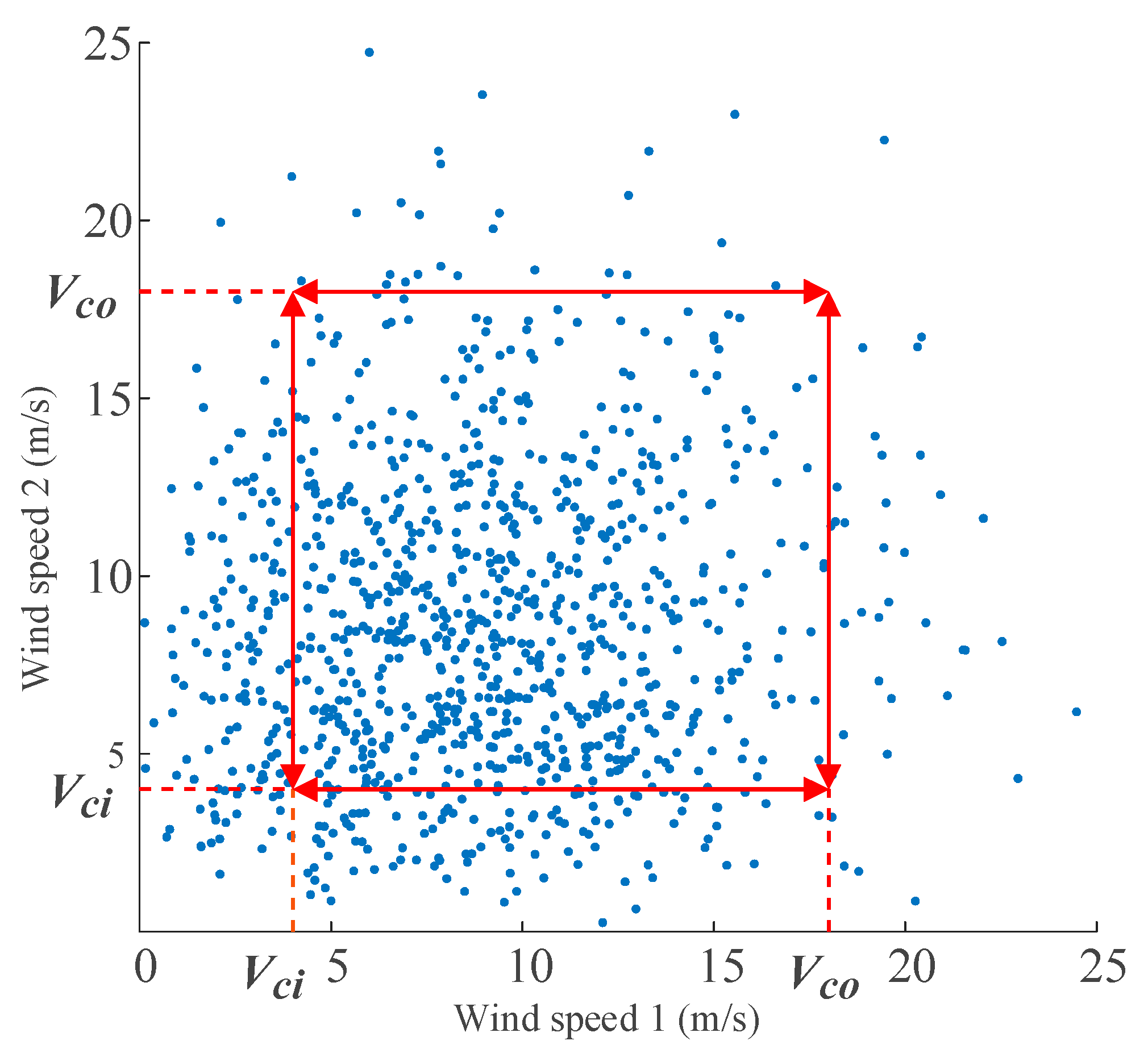
Most MCM algorithms sample the whole random variable distribution interval. This paper presents the concept of a desired range. A desired range is a reduced sampling space and samples collected in this sampling space are more helpful to PLF calculations than those collected outside the range. Usually, the selection of the desired range needs to consider the actual situation, such as the condition of random variables or calculation purpose. For example, a wind turbine is often shut down or disconnected when wind speeds exceed the threshold. Suppose the limited speed is $V_{\mathrm{ci}}$ to $V_{\mathrm{co}}$, Figure 1 shows some samples of wind speeds collected from two wind farms (WF) in the same period of time. The abscissa and ordinate denote the wind speeds as WF1 and WF2, respectively.

Obviously, many invalid samples are located outside the range of $V_{\mathrm{ci}}$ to $V_{\mathrm{co}}$. Therefore, in one case, we put the sampling range in the range of $V_{\mathrm{ci}}$ to $V_{\mathrm{co}}$ or even in a smaller range to improve the efficiency of the sampling. If a group of discrete samples is in the desired range, these samples are used as important samples. In addition, we are often concerned with whether the current in important lines exceeds the limitation after DG access. If the current exceeds the limitation, the operation of grid needs to be adjusted. Therefore, in order to analyze the over-limit probability of important lines, the desired range can be placed near the line limit value. Similarly, if the resulting current value of PLF is in the vicinity of the limit value, this group of discrete samples is selected as the “important samples”. The specific range is set out in the simulation in Section 3.

Here, we address the second problem in ISM. A new probability distribution function with the same probability properties of the original one is needed. In particular, the following principle was introduced to keep the new random variable with the same expectation and smaller variance of the old one.

The probability of the original random variable $Z$ was $p\left(z\right)$. $h\left(z\right)$ is another probability density function regarding z, which we call important distribution function (IDF). According to the characteristics of probability density function, ${\displaystyle \sum }_{z\in Z}h\left(z\right)=1$. Supposing the new function $g^{*}\left(z\right)$:

$$g^{*}\left(z\right)=\frac{g\left(z\right)p\left(z\right)}{h\left(z\right)}$$

(1)

where $g\left(z\right)$ is used to represent the power flow equation (the Newton–Raphson method).

Theorem 1.

$g\left(z\right)$and$g^{*}\left(z\right)$share the same mean but different variances.

Proof of Theorem 1.

$$E\left(g^{*}\left(z\right)\right)={\displaystyle \sum }_{z\in Z}\frac{g\left(z\right)p\left(z\right)}{h\left(z\right)}\cdot h\left(z\right)={\displaystyle \sum }_{z\in Z}g\left(z\right)p\left(z\right)=E\left(g\left(z\right)\right)$$

(2)

$$\begin{gathered} D\left(g^{*}\left(z\right)\right)=E{\left[g^{*}\left(z\right)-E\left(g^{*}\left(z\right)\right)\right]}^2=E{\left[\frac{g\left(z\right)p\left(z\right)}{h\left(z\right)}-E\left(g^{*}\left(z\right)\right)\right]}^2 \\ =h\left(z\right)\cdot {\displaystyle \sum }_{z\in Z}{\left[\frac{g\left(z\right)p\left(z\right)}{h\left(z\right)}-E\left(g\left(z\right)\right)\right]}^2 \end{gathered}$$

(3)

 ☐

Equations (2) and (3) show that we can use a new random variable, $g^{*}\left(z\right)$, to replace the original random variable, $g\left(z\right)$. Here, $h_z\left(z\right)=\frac{g\left(z\right)p\left(z\right)}{E\left(g\left(z\right)\right)}$ is an ideal situation of $h\left(z\right)$, and we named it as the optimal IDF. In this situation, $D\left(g^{*}\left(z\right)\right)=0$, so that the means of $g^{*}\left(z\right)$ would be obtained by only one sampling. However, $E\left(g\left(z\right)\right)$ cannot be solved because variable Z is a continuous random variable. Thus, we use sample reconstruction to approach the optimal IDF. Next, a non-parametric reconstruction method based on kernel function is adopted.

2.2. Reconstruction of Optimal Important Distribution Function Based on Non-Parametric Estimation

This section introduces the non-parametric reconstruction based on the kernel function to approach the optimal IDF.

Z₁, Z₂, Z₃, …, Z_M are the important samples collected from variable Z. ${\widehat{h}}_z\left(Z\right)=\frac{1}{{\mathrm{Mh}}_n}{\displaystyle \sum }_{i=1}^{M}K\left(\frac{z-Z_i}{h_M}\right)$ is called the reconstructed distribution function (RDF), where function K(z) is the kernel function and h_M is the bandwidth of K(z). M is the number of samples. The properties of the kernel function are given in Reference [23], and proved that the value of h_M determines the similarity between RDF and optimal IDF. We used a Gaussian distribution to replace K(z):

$${\widehat{h}}_z\left(z\right)=\frac{1}{{\mathrm{Mh}}_M}{\displaystyle \sum }_{i=1}^M\left(\frac{1}{\sqrt{2\mathsf{\pi }}}{e}^{-\frac{1}{2}{\left(\frac{z-Z_i}{h_M}\right)}^2}\right)$$

(4)

The method of integral square-error (ISE) was adopted for the choosing optimal bandwidth. Define ISE as:

$$\mathrm{ISE}\left({\widehat{h}}_z\left(z\right)\right)=\int {\left({\widehat{h}}_z\left(z\right)-h_z\left(z\right)\right)}^2\mathrm{dz}=\int \left({\widehat{h}}_z^2\left(z\right)-2{\widehat{h}}_z\left(z\right)h_z\left(z\right)+h_z^2\left(z\right)\right)\mathrm{dz}$$

(5)

Optimal bandwidth h_M is what made $\mathrm{ISE}\left({\widehat{h}}_z\left(z\right)\right)$ the smallest. In order to simplify the calculation, we performed some approximate processing for Equation (5). Firstly, the last item $h_z^2\left(z\right)$ was independent from h_M; thus, we focused on the first two items of $\mathrm{ISE}\left({\widehat{h}}_z\left(z\right)\right)$. Supposing:

$$R\left({\widehat{h}}_z\left(z\right)\right)=\int {\widehat{h}}_z^2\left(z\right)\mathrm{dz}-2\int h_z\left(z\right){\widehat{h}}_z\left(z\right)=R_1-2R_2$$

(6)

where $R_1=\frac{1}{M^2}{\displaystyle \sum }_{i,j}^M\frac{1}{\sqrt{2\mathsf{\pi }{h}_M^2}}{e}^{-\frac{1}{2}{\left(\frac{Z_i-Z_j}{h_M}\right)}^2}$, and the second term, R₂, can be derived from the samples collected by the small-scale Monte-Carlo sampling in the desired range:

$$R_2={\widehat{h}}_z\left(z\right)h_z\left(z\right)=E\left[\widehat{h}\left(z\right)\right]\approx \frac{1}{M}{\displaystyle \sum }_{i=1}^M{\widehat{h}}_{-i}\left(Z_i\right)$$

(7)

where ${\widehat{h}}_{-i}\left(Z_i\right)=\frac{1}{M-1}{\displaystyle \sum }_{j=1,j\ne i}^M\frac{1}{\sqrt{2\mathsf{\pi }}{h}_M}{e}^{-\frac{1}{2}{\left(\frac{Z_i-Z_j}{h_M}\right)}^2}$. The −i that exists in the subscript represents that it is not contained in the ith item in the sum. Details of the approximation in Equation (8) are in the following:

$$E\left[\frac{1}{M}{\widehat{h}}_{-i}\left(Z_i\right)\right]=\frac{1}{M}{\displaystyle \sum }_{i=1}^M{E}_{Z_i}\left[{\widehat{h}}_{-i}\left(Z\right)\right]=E_z\left[{\widehat{h}}_{-i}\left(Z\right)\right]=\int \widehat{h}\left(z\right)h\left(z\right)\mathrm{dz}$$

(8)

Then, bringing these results to Equation (6),

$$R\left(\widehat{h}\left(z\right)\right)=\frac{1}{M^2}{\displaystyle \sum }_{i,j}^M\frac{1}{\sqrt{2\mathsf{\pi }{h}_M^2}}{e}^{-\frac{1}{2}{\left(\frac{Z_i-Z_j}{h_M}\right)}^2}-\frac{2}{M}{\displaystyle \sum }_{i=1}^M{\widehat{h}}_{-i}\left(Z_i\right)$$

(9)

Finally, we get an ideal bandwidth by minimizing the value of Equation (9). The RDF was also calculated in sequence.

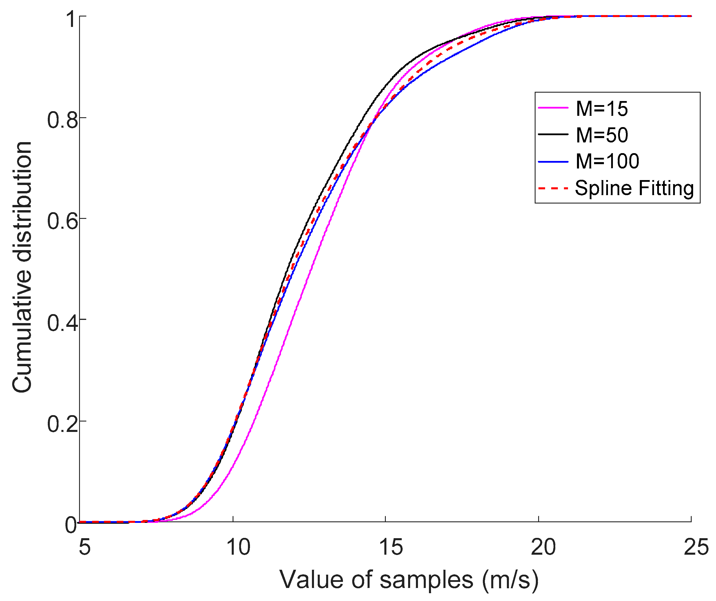
To study the effect of M on the accuracy of RDF, some samples in different M were selected from 2000 wind speed samples in a certain range, and constructed according to Equations (5)–(9). The probability distribution curves of the IDF constructed using different M are compared in Figure 2, and we took the spline fitting curve as the standard distribution curve.

As shown in Figure 2, the curve in M = 100 is very close to the standard distribution curve. Therefore, we used M = 100.

2.3. Latin Hypercube Sampling with Cholesky Decomposition Method

After obtaining the RDF of each new variable, we adopted LHS to sample the new random variable. Then, Cholesky decomposition was used to minimize the correlation of samples, which was sampled using LHS.

LHS is a stratified sampling method based on the Monte-Carlo method; the range of cumulative distribution function F_k(Z) is divided into N intervals, in which the representative sample is extracted to replace the whole sampling range. LHS can greatly improve the efficiency of sampling, especially the accuracy of an algorithm under low sampling times. The details of the sampling steps of LHS has been given in Reference [18]. In this way, an original sampling matrix, $Z_0\left(n\times N\right)$, which contains a correlation is obtained. The number of input random variables was n, and the times of LHS sampling was N. The next process is to reorder the $Z_0$ for its minimal correlation by using the Cholesky decomposition method. The detailed theory and related proofs of the Cholesky decomposition method are as follows:

Let $C_Z$ be the correlation coefficient matrix of input random variables Z₁, Z₂, Z₃, …, Z_M.

$$C_Z=\left[\begin{array}{cccc}1& {\rho }_{12}& \cdots & {\rho }_{12}\\ {\rho }_{12}& 1& \cdots & {\rho }_{12}\\ ⋮& ⋮& \ddots & ⋮\\ {\rho }_{12}& {\rho }_{12}& \cdots & 1\end{array}\right]$$

(10)

where ${\rho }_{ij}$ is the correlation coefficient of Z_i and Z_j.

There is a set of standard normal random variables, E₁, E₂, …, E_n, with a one-to-one mapping between E_n and Z_n:

$$E_k={\Phi }^{-1}\left(F_k\left(Z_k\right)\right),k=1,2,\cdots ,n$$

(11)

Accordingly, let the correlation coefficient matrix of E₁, E₂, …, E_n be $C_E$.

$$C_E=\left[\begin{array}{cccc}1& {\rho }_{12}^{\text{'}}& \cdots & {\rho }_{1n}^{\text{'}}\\ {\rho }_{21}^{\text{'}}& 1& \cdots & {\rho }_{2n}^{\text{'}}\\ ⋮& ⋮& \ddots & ⋮\\ {\rho }_{n1}^{\text{'}}& {\rho }_{n2}^{\text{'}}& \cdots & 1\end{array}\right]$$

(12)

Off-diagonal elements of $C_E$ also have a one-to-one mapping with $C_X$:

$${\rho }_{ij}=G\left({\rho }_{ij}^{\text{'}}\right)\cdot {\rho }_{ij}^{\text{'}}$$

(13)

where conversion coefficient $G\left({\rho }_{ij}^{\text{'}}\right)$ can be obtained by numerical integration and the search method in Reference [24]. The empirical expression of $G\left({\rho }_{ij}^{\text{'}}\right)$ was given in Reference [25].

Then, perform Cholesky decomposition for $C_E$:

$$C_E={\mathrm{BB}}^T$$

(14)

Assuming that vector Y consists of n independent random variables, $Y_i$ (i = 1, 2, …, n), that obey standard normal distribution, let:

$$M=\left[\begin{array}{c}{M}_1\\ ⋮\\ M_n\end{array}\right]=\mathrm{BY}=\left[\begin{array}{ccc}{b}_{11}& & \\ ⋮& \ddots & \\ b_{n1}& \dots & b_{\mathrm{nn}}\end{array}\right]\times \left[\begin{array}{c}{Y}_1\\ ⋮\\ Y_n\end{array}\right]$$

(15)

Theorem 2.

In Equation (15), $M_1$, $M_2$, …, $M_n$obey the standard normal distribution.

Proof of Theorem 2.

The linear combination of standardized normal random variables also obeys the standard normal distribution. For any variables, $Z_i$ (i = 1, 2, …, n), there is

$$E\left(Z_i\right)=E\left({\displaystyle \sum }_{j=1}^i{b}_{ij}\cdot Y_j\right)={\displaystyle \sum }_{j=1}^i{b}_{ij}\cdot E\left(Y_j\right)=0$$

(16)

The correlation coefficient matrix of $Z_1$, $Z_2$,…, $Z_n$ is:

$$\rho \left({\mathrm{ZZ}}^T\right)=\rho \left({\mathrm{BYY}}^T{B}^T\right)=B\cdot \rho \left({\mathrm{YY}}^T\right)\cdot B^T={\mathrm{BB}}^T=C_E$$

(17)

 ☐

Therefore, we performed random sampling for M, obeying the standardized normal distribution and obtained $M^{*}$ as the order matrix. Then, the original sampling matrix using LHS was arranged according to the order of elements in $M^{*}$, and the final sample matrix was obtained.

3. Performance Analysis

To investigate the performance of the LHISM method, a modified IEEE-30 bus system [26] was used in the MATLAB platform (2016b, The MathWorks, Inc., Natick, MA, USA). Firstly, the steps of LHISM were given and then we set the input variables and the desired range for two different situations. The simulation results and analyses are presented.

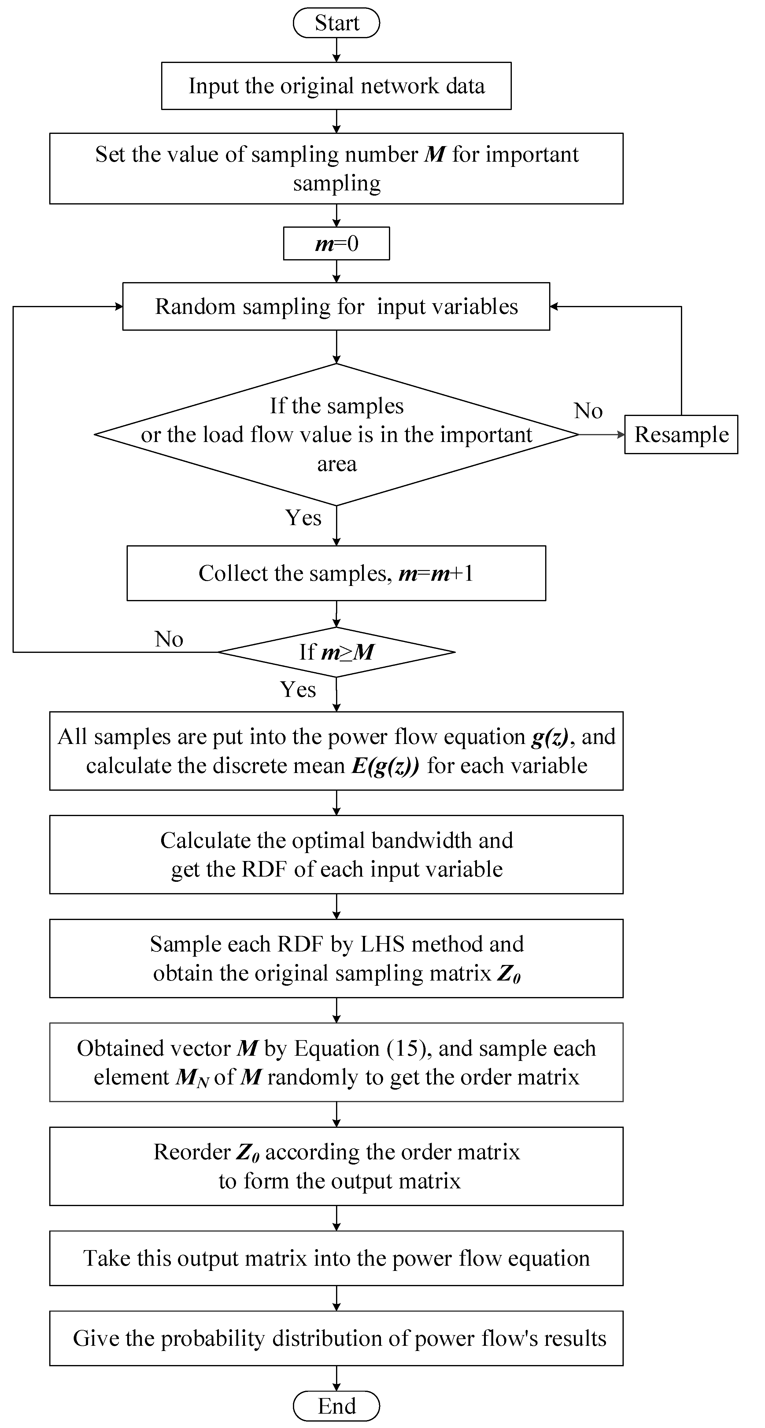
3.1. Steps

● STEP 1:

The first step was to set parameters. The wind speed of each wind farm was taken as a random variable. The desired range and input the value of M of the required samples was set.

● STEP 2:

The second step was to obtain important samples. Single random sampling was done for random variables. If the samples or according load flow values of samples were located in the desired range, these samples were taken as important samples. This step was repeated until each random variable collected M important samples.

● STEP 3:

The third step was to obtain reconstructed distribution functions (RDFs). The discrete means of each random variable were obtained by taking the important samples in the power flow calculation equation. Then, the optimal bandwidth was calculated and the RDFs for each input variable were acquired.

● STEP 4:

The fourth step was to use the LHS and Cholysky method to sample the data and address the correlation problems. Each RDF was processed using LHS to generate $Z_0\left(n\times N\right)$, and vector M was formed according to the Cholesky decomposition method, and M was randomly sampled to form order matrix $M^{*}$, then the order matrix was used to reorder $Z_0$ and get the final sample matrix.

● STEP 5:

The last step was to carry out a deterministic power flow calculation and data analysis of the results. The power flow was calculated using the final sample matrix. Then, the statistical results and the probability distribution of the power flow were obtained. Finally, the corresponding conclusions of power flow were given.

A flowchart of the LHISM algorithm is shown in Figure 3.

3.2. The Setting of Desired Range

The active output (P_W) model of a single wind turbine can be simplified as a piecewise function, as shown in Equation (18):

$$P_W=\{\begin{array}{ll}0& V_s<V_{\mathrm{ci}}\mathrm{or}{V}_s>V_{\mathrm{co}}\\ P_{\mathrm{WR}}\frac{V_s-V_{\mathrm{ci}}}{V_r-V_{\mathrm{ci}}}& V_{\mathrm{ci}}\le V_s<V_r\\ P_{\mathrm{WR}}& V_r\le V_s\le V_{\mathrm{co}}\end{array}$$

(18)

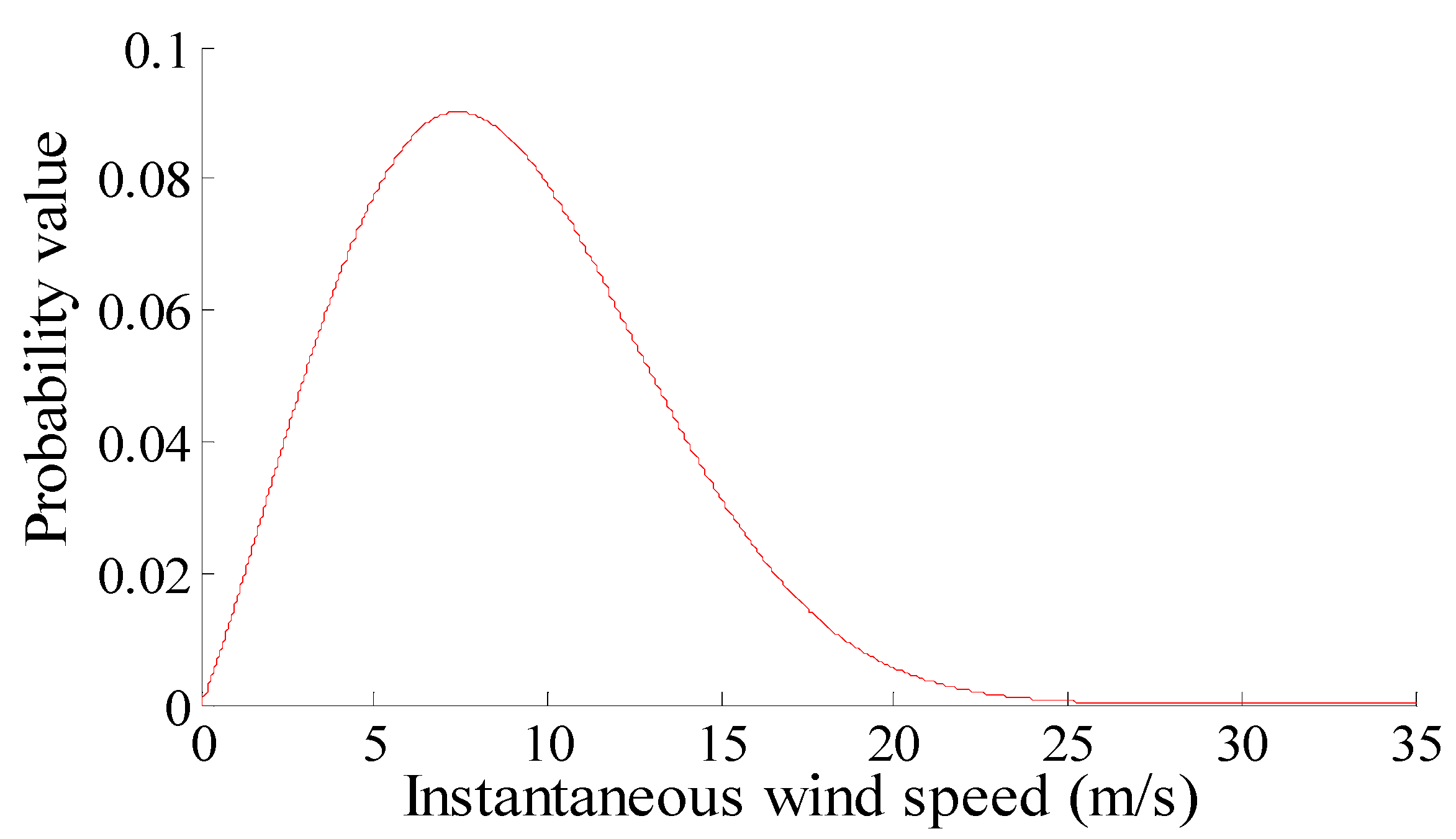
where $P_{\mathrm{WR}}$ is the active output of the wind turbine, and $P_{\mathrm{WR}}$ is the rated power. $V_s$ is the wind speed; $V_{\mathrm{ci}}$, $V_r$, $V_{\mathrm{co}}$ are the cut-in wind speed, rated wind speed, cut-out wind speed, respectively. In practice, a Weibull distribution is usually used to model instantaneous wind speeds. The curve of the probability distribution of the instantaneous wind speeds, which is modeled using a Weibull distribution, is given in Figure 4. Its scale parameter is 10 and the shape parameter is 2.15.

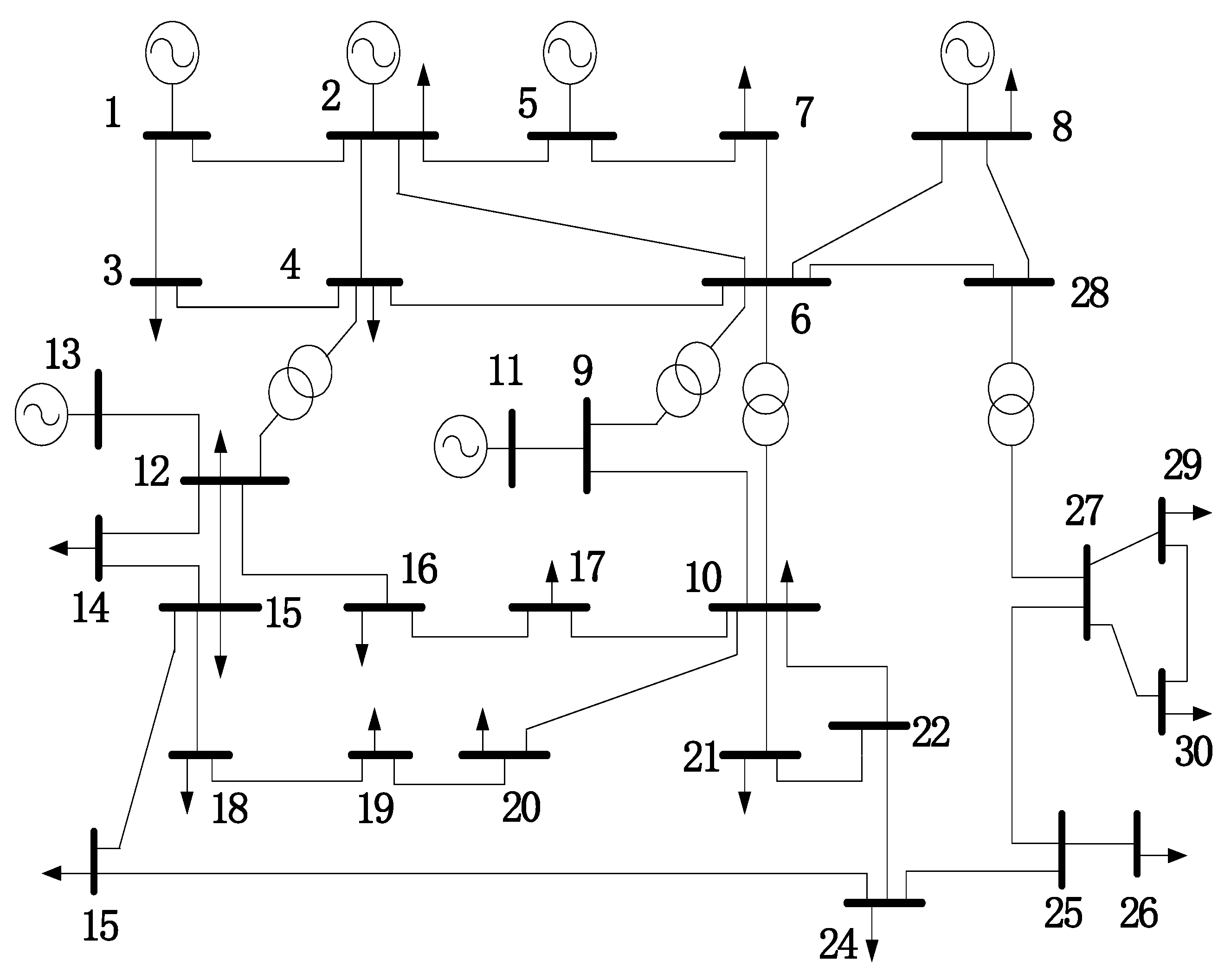
As shown in Figure 5, an IEEE-30 bus system is modified for simulation analyses.

Nodes 14, 15, 16, 17, 18 are linked to a wind farm (WF), and the rated capacity of each WF is $P_{\mathrm{WR}}=40\mathrm{MV}$. $V_{\mathrm{ci}}$, $V_r$, $V_{\mathrm{co}}$ are the cutting wind speed, rated wind speed, and cutting speed. Their values are 2.5, 12, and 20 m/s, respectively.

The correlation coefficient matrix of the five WFs is:

$$C_Z=\left[\begin{array}{ccccc}1.0& 0.5& 0.8& 0.7& 0.6\\ 0.5& 1.0& 0.7& 0.6& 0.8\\ 0.8& 0.7& 1.0& 0.5& 0.6\\ 0.7& 0.6& 0.5& 1.0& 0.9\\ 0.6& 0.8& 0.6& 0.9& 1.0\end{array}\right]$$

(19)

1. Situation I:

As described in Section 2, when the wind speed is lower or higher than a threshold, power generation is often shut down or disconnected. Therefore, this situation determines whether a sample of wind speed is in the desired range, determined by its output power:

$$0.3P_{\mathrm{WR}}\le P_W\le P_{\mathrm{WR}}$$

(20)

2. Situation II:

In situation II, the main consideration was the current values of the main lines after DG access. For example, this simulation only considered the limitation of the current of the line between node 3 and node 4.

$$\{\begin{array}{c}{I}_L=1.3p.u.\\ 0.9I_L\le I_{34}\le 1.1I_L\end{array}$$

(21)

I₃₄ is the actual current of the line between node 3 and node 4, and I_L is maximum allowable current for this line. If the actual current conforms to Equation (21), the corresponding wind samples are regarded as important samples.

3.3. Simulation Result of Situation I

The aims of a power flow calculation usually include a line’s active power (P), a line’s reactive power (Q), a node’s voltage (V), and the angle of voltage and current, $\theta$.

This example takes the result of MCM simulation with 20,000 sampling as the standard value of PLF. The standard value of the statistical mean and standard deviation are expressed as ${\mu }_a$ and ${\sigma }_a$. The statistical mean and standard deviation of sample are expressed as ${\mu }_s$ and ${\sigma }_s$, respectively. Accordingly, the accuracy of the LHISM algorithm can be estimated by the relative error rate (RET):

$${\mathrm{RET}}_{\mu }=\left|\frac{{\mu }_a-{\mu }_s}{{\mu }_a}\right|\times 100\%$$

(22)

$${\mathrm{RET}}_{\sigma }=\left|\frac{{\sigma }_a-{\sigma }_s}{{\sigma }_a}\right|\times 100\%$$

(23)

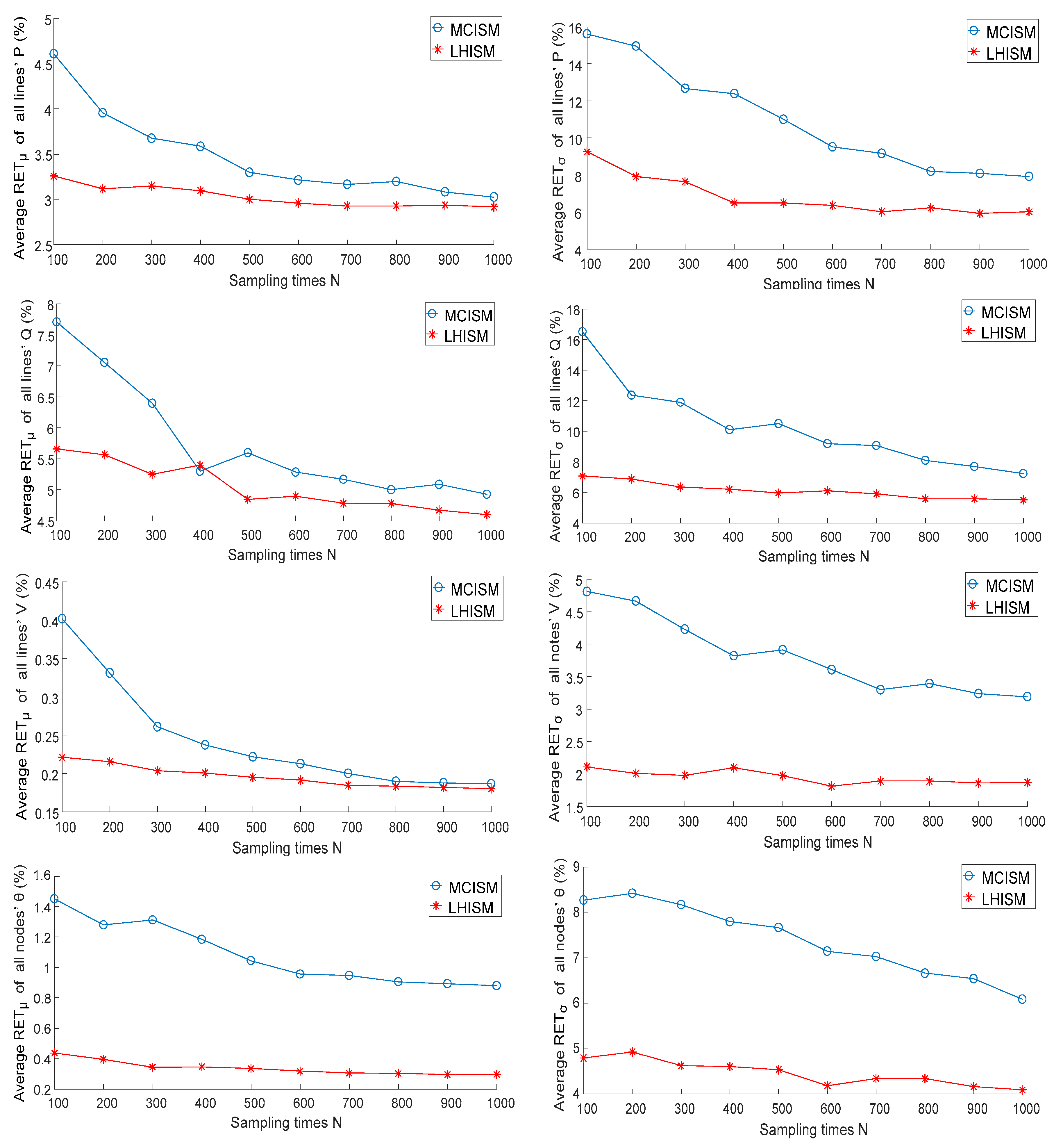
Set M = 100, and follow the steps described in Figure 4 under the Situation I. In order to show the performance of LHISM, MCM sampling in the desired range was adopted for comparison. The contrast algorithm is referred to as the Monte-Carlo important sampling method (MCISM). Ten simulations were carried out using the same data and settings. The average RETs of these simulations are shown in Figure 6.

The following three conclusions are drawn from Figure 6:

• LHISM had a higher accuracy compared with MCISM, especially for the results of P and $\theta$. The mean accuracy of LHISM was more than 60% higher than that of MCISM in the case of small sampling times (N = 100) and was about 10% higher in the case of large sampling times (N = 1000).
• Compared with the traditional MCM, LHISM has a very high accuracy in calculating the standard deviation of tidal current results. The precision of the standard deviation obtained using LHISM was more than 40% higher than that of the traditional method, both in terms of small or large sampling times.
• LHISM had a more stable accuracy than MCISM. The variation in LHISM errors between high sampling times and low sampling times was not more than 30%, and was under 35–50% in MCISM.

3.4. Simulation Result of Situation II

In Situation II, the cumulative distribution curve of current I₃₄ was obtained by sampling LHS 500 times. The curve was also compared with the results of the MCM simulation with 20,000 sampling.

Figure 7 shows that the probability of exceeding the limit of I₃₄ was 14.9% using LHISM. If the limiting probability obtained by the MCM simulation is regarded as the standard value, the RET is only 5.65%.

Assume the reliable average RET of limiting probability is 0.1%. The LHS algorithm in Reference [19] was used as a comparison. The sampling times and the computation times required for the two methods for achieving a reliable average error are given in

Table 1. Comparison of sampling times and calculation times of the two methods.

Method	Sampling Times	Calculation Time (s)
LHISM	407	732
LHS-Copula	789	1503

.

Table 1 shows that LHISM took less time to compute compared with the LHS method, and the computing speed of LHISM was about twice as fast as that of the LHS method.

4. Conclusions

A novel PLF method called LHISM has been proposed in this paper, based on ISM and the modified LHS method. In ISM, the sampling space is narrowed to the desired range. In addition, a new random variable that retains the probability characteristics of the original random variable is constructed using non-parametric estimation. The smaller variances of the new random variables contribute to improving the sampling efficiency. Then, modified LHS are introduced to improve the accuracy under low sampling times and the speed of correlation processing.

The advantage of LHISM is that it, not only keeps the advantages of LHS, such as accuracy with low sampling times, but also further narrows the sampling range. In addition, a simpler method for correlation processing is also applied. Our simulations verified that LHISM has a higher accuracy and computational efficiency compared with the MCM algorithm, especially with short sampling times. In practical applications, LHISM can evaluate the power flow limit after DG access, with a shorter computation time than the LHS method.

Due to the limitations of data, this paper only considered a grid model with fan access. The principle of this algorithm is also applicable to other distributed generation grids, but it needs some samples to verify its performance. Further research is needed to extend the algorithm to hybrid generation models, such as power systems with wind, light, and biomass energy.