Computational Fluid Dynamics Modelling and Simulation of an Inclined Horizontal Axis Hydrokinetic Turbine


1
PAI+ Group, Energetics & Mechanics Department, Faculty of Engineering, Universidad Autónoma de Occidente, 760030 Cali, Colombia
2
Computational Mechanics Research Group, Mechanical Engineering Department, Faculty of Engineering, Universidad de los Andes, 111711 Bogotá, Colombia
*
Author to whom correspondence should be addressed.
Energies 2018, 11(11), 3151; https://doi.org/10.3390/en11113151
Submission received: 2 August 2018
/
Revised: 25 October 2018
/
Accepted: 30 October 2018
/
Published: 14 November 2018
(This article belongs to the Section A: Sustainable Energy)
Abstract
:In this contribution, unsteady three-dimensional numerical simulations of the water flow through a horizontal axis hydrokinetic turbine (HAHT) of the Garman type are performed. This study was conducted in order to estimate the influence of turbine inclination with respect to the incoming flow on turbine performance and forces acting on the rotor, which is studied using a time-accurate Reynolds-averaged Navier-Stokes (RANS) commercial solver. Changes of the flow in time are described by a physical transient model based on two domains, one rotating and the other stationary, combined with a sliding mesh technique. Flow turbulence is described by the well-established Shear Stress Transport (SST) model using its standard and transitional versions. Three inclined operation conditions have been analyzed for the turbine regarding the main stream: 0° (SP configuration, shaft parallel to incoming velocity), 15° (SI15 configuration), and 30° (SI30 configuration). It was found that the hydrodynamic efficiency of the turbine decreases with increasing inclination angles. Besides, it was obtained that in the inclined configurations, the thrust and drag forces acting on rotor were lower than in the SP configuration, although in the former cases, blades experience alternating loads that may induce failure due to fatigue in the long term. Moreover, if the boundary layer transitional effects are included in the computations, a slight increase in the power coefficient is computed for all inclination configurations.
1. Introduction
Climate change, associated with negative impacts resulting from overexploitation and the use of fossil fuels, has not only induced environmental problems of great magnitude but has also generated an awakening in the scientific community and governments. All interested actors agree today that an alternative solution to the increasing energy deficit is the use of renewable energies [1]. Therefore, using hydrokinetic energy as a renewable source for generating electricity is nowadays one of the most active fields of research [2].
Water currents such as oceans and rivers constitute a wide and almost unexploited source for renewable energy generation. According to Reference [3], a representative electricity generation can be obtained by the ocean energy industry and the forecast for the year 2025 is to reach up to 200 GW of installed generation capacity. On the other hand, many developing countries are crossed by rivers which carry significant volumetric water flow along the year. This fact could be a revolutionary scenario for remote populations which could use this energy source if effective and low-cost energy harnessing mechanisms are developed [3]. Around the world there are more than 300 hydrokinetic projects already in process, divided into four main types of technologies: ocean wave, tidal stream, ocean current and river hydrokinetic [3]; many of the applications in marine environments are for the large-scale, while, the river and channels applications are for the small-scale [4].
Because of its predictability, the large density of energy, and the low environmental impact (scarce visual impact, no emissions, no noise), the kinetic energy present in water streams (oceans, rivers, or tidal channels) has received considerable attention in recent years [3,4,5]. Such kinetic energy can be extracted through properly designed immersed turbines [6] without the need of large facilities as reservoirs or dams. As it generates no emissions, the environmental impact is minimal. Compared to other hydraulic technologies, the site selection is much less restrictive and because it does not require significant infrastructure, the implementation time is short and the initial costs are reduced. Moreover, the modular character of hydraulic power enables scalable output energy, allowing for a reduction of the energy cost per kW. Another advantage is related with the continuous flow of water in oceans and rivers which eliminates the need for storing the energy, which is a crucial benefit for remote communities and very convenient in public services [6].
From the technical point of view, the conversion of kinetic energy present in large rivers, tides, and ocean currents involves two processes. The first process implies that the energy available on tidal, ocean or river currents must be extracted and converted into mechanical energy at the rotor axis, and the second process deals with converting such mechanical energy into electricity using a generator [7]. However, despite all the performed research and experiments, the study of hydrokinetic turbines (concentrated mainly in the primary process), is still in an incipient state due to the complexity and cost that represents a suitable testing bench to operate this kind of rotors. That is, the reason why the main part of its design is based on the analogy with wind turbines. Moreover, the majority of the developed innovations have been the result of empirical studies conducted in order to deal with anchoring systems, channels, debris protection, and maintenance [8].
Flow dynamics in the horizontal axis hydrokinetic turbines (HAHT) is complex and has attracted the interest of the scientific community during the last years, specifically aimed to understand their performance and to improve efficiencies. To reach such objectives, a deep understanding of the involved hydrodynamics is required. In that sense, since a few years ago, Computational Fluid Dynamics (CFD) has become an essential approach for describing the fluid flow behavior around hydro turbines. CFD numerically solves the governing equations of Fluid Mechanics (i.e., mass, momentum, and energy conservation) in complex geometries in a general framework. Due to its advantages over other simplified methods [9], it has been the approach adopted in the present study and, in the following analysis, several recent studies that employ CFD to investigate different aspects of the design, development, and operation of HAHT’s are described.
Kang et al. [10] conducted a numerical study with two kinds of geometry composed of a rectangular box and a rotating domain; in the first case they only analyzed the rotor, while in the second case the complete structure (rotor and mounting) was analyzed to determine the effect of the support in the turbine hydrodynamic efficiency. The results of these authors illustrated the flow complexity and showed that the extracted power of the full turbine mainly depends on the rotor geometry and the TSR (Tip Speed Ratio), as they were not very affected by the mounting components of the turbine and the channel bed. The authors carried out an experimental analysis used to validate the CFD results; they found that the refined grid presented a discrepancy at the power coefficient less than 5%, which is considered quite satisfactory taking into account that measurements were carried out for the complete turbine geometry including an ambient turbulence in the site. In Reference [11], the authors wanted to identify the main design parameters affecting the performance of a Horizontal Axis Water Turbine by presenting numerical results in comparison with experimental measurements. In such work, it was demonstrated that, when the other parameters were kept constant, the numerical output power of the turbine was roughly proportional to the square of the blade span and to the cube of the incoming velocity. Regarding the blade number, the authors found that the optimum number was three and that an increase beyond that caused a decrease in power production. Again, the authors validated the simulation with experimental data obtaining a difference of power coefficient between experimental and numerical results lower than 15%; the discrepancy could be attributed to the generator losses and possible measuring errors. Guo et al. [12] used a three-dimensional CFD simulation to analyze the turbulent flow characteristics in the velocity field up and downstream of the turbine and the effects of a discrete number of blades. Motivated by its use in BEM (Blade Element Momentum theory), the authors derived the flow induction factors (axial and tangential) at several locations downstream of the rotor from their CFD results. It was concluded that the main induced velocity component by the vortices was the axial component. Additionally, the computations showed that vortices developed at the tip of each blade induced a down-wash velocity near the rotor and generated an azimuthal variation of velocity components; these are responsible for the appearance of flow non-uniformities upstream and downstream the rotor. The authors concluded that the calculation model used provided an acceptable accuracy because the differences between the numerical results and experimental values of power and thrust coefficients were lower than 5%.
With the objective of reducing the computational effort of CFD, some authors have coupled BEM and CFD. In this context, BEM, using the hydrofoil characteristics in two dimensions, can be employed to predict the hydrodynamic performance of a hydrokinetic turbine, while the CFD coupled with BEM take into account three dimensions using an actuator disc which in addition to predicting the performance also allows us to predict wake features of the turbine; however, these estimations do not include the rotating blades and are not able to predict some details of the flow field. For instance, Reference [13] present a usable tool which was applied to predict the behavior of tidal stream turbines in typical offshore conditions. The obtained results were satisfactory because the comparison of the power coefficient estimation by BEM-CFD with experimental data showed a difference between 0.3% and 8.8%. As another example of the coupling BEM-CFD, Reference [14] concludes that the BEM-CFD results of the hydrokinetic turbine were able to accurately predict the thrust; however, the power was overestimated. This behavior was present at lower values of TSR. In particular, the BEM-CFD calculations provided a fairly good approximation to the near rotor circumferentially averaged fluid velocity with the exception of the tip vortices [14].
In Reference [15] the authors reviewed and compared results from various models of horizontal axis water turbines at different spatial resolutions; the aim of the study was to investigate the effect of small variations in lift and drag characteristics of the hydrofoils employed in the blade design on the turbine performance. They found that from a practical perspective, relatively small changes on the blade aerodynamic properties are improbable to cause a significant decrease in the performance. However, such modifications had the effect of altering the value of the optimum power coefficient as well as the tip speed ratio at which it is achieved. Understanding the behavior of turbine wakes is crucial if turbines are to be deployed in arrays; for such reason, a comparison between BEM-CFD and full CFD method was focused on determination of velocity deficit in the turbine wake. When comparing with experimental data, Reference [15] found that both models captured reasonably well the wake dynamics, although there was around a 5% difference between both predictions. Reference [16] presented comparisons between experiments and CFD numerical computations focused on the velocity profiles in the wake region of a HAHT. The agreement between them was very reasonable, showing the same predicted wake recovery trend. Moreover, the turbine closeness to the water surface promoted the flow modification around the turbine which affected the wake development downstream the rotor. Finally, supported by the presented results, Zhang et al. [16] claimed that CFD is an appropriate tool to simulate the performance of tidal turbines and that the turbine proximity to the water surface influences the wake recovery.
In a HAHT, the lowest pressure near the blade tip is due to the high revolution speed around these sections. Therefore, the accurate description of the flow field near the blade tip becomes important for two reasons: to analyze the turbine power performance and because cavitation is prone to occur in these areas, which of course alters turbine efficiency [17]. Following Reference [4] in order to design a high-performance rotor, the cavitation and pressure coefficient should be as low as possible while the lift to drag ratio should be kept high. In particular, Lee et al. [17] introduced a new blade design for horizontal water rotors that included a raked tip shape aimed to noise reduction and cavitation inception delay. The concept was evaluated by numerical CFD simulations showing positive results in delaying cavitation without degrading the turbine efficiency.
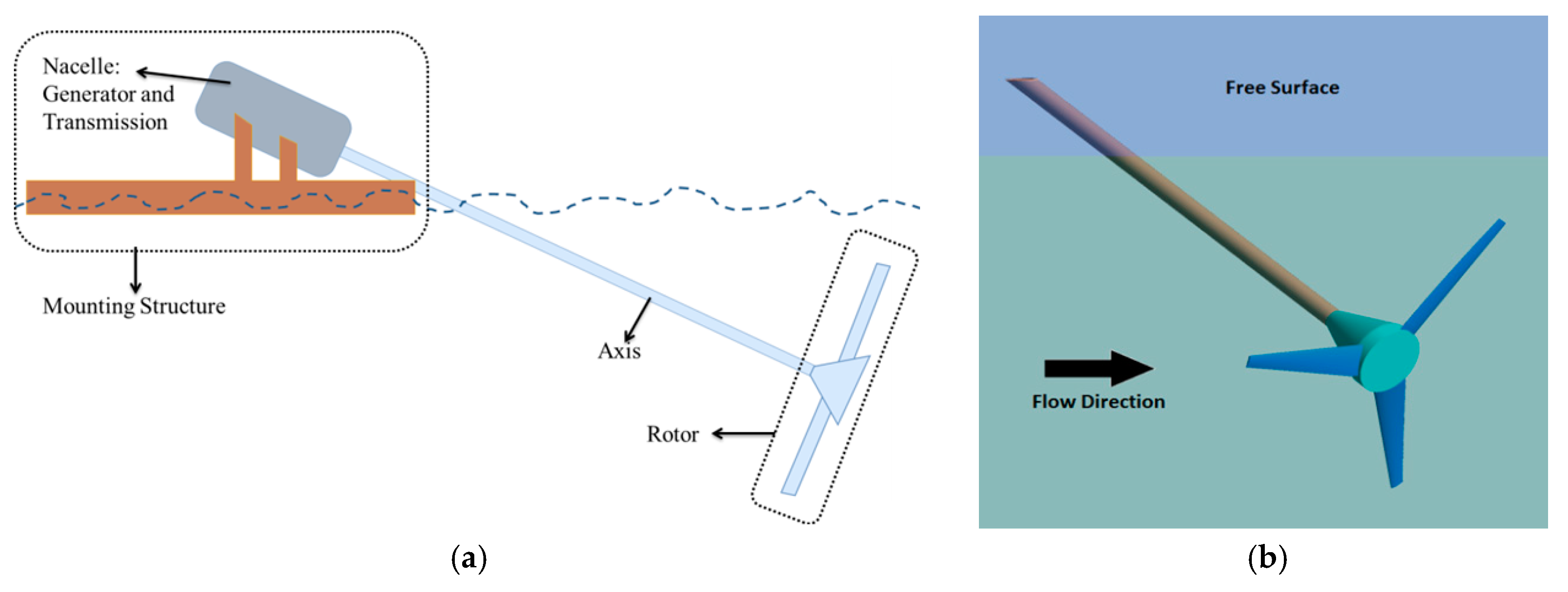
The present contribution deals with the performance estimation of small HAHT’s of Garman type using CFD. The arrangement of such turbines can be appreciated in Figure 1b: the turbine is assembled in a floating structure on a channel or river operating with its axis inclined regarding the flow direction. As it was mentioned, the main use of this kind of turbines is to provide electricity to isolated communities so their design has been essentially empirical and only a few experimental studies have appeared [18,19]. For instance, Al Mamun [18] performed experiments on a laboratory Garman turbine with three blades operating with an inclination of 45° with respect to the main channel flow direction. Experiments were conducted for three incoming speeds and two pitching angles aimed to analyze the turbine performance versus tip speed ratio. As a result, a power coefficient of around 30% was reached. However, no reports about the CFD analysis of inclined HAHT’s have been found in the literature. Therefore, the authors believe that, to the best of their knowledge, this is the first time in which the CFD simulation of the hydrodynamic behavior of a HAHT which operates with an inclined axis respect to the main stream is attempted.
This paper is structured in the following way. After the introduction, the considered geometrical configurations and the meshing process are described in Section 1. The numerical simulation methodology and the key parameters governing the operation of HAHT’s are summarized in Section 2. The obtained results for the non-dimensional turbine coefficients are presented in Section 3 which are organized in several subsections: their behavior along a turbine revolution is described first and later the analysis is extended to build the respective curves versus tip speed ratio; moreover, the effects of including the modeling of the transitional behavior of the boundary layer on turbine performance are discussed in Section 4.3. Comparison of the computed CFD results with available experimental data and those obtained with more simplified models is performed in Section 4; also, in this section, a comparison of additional CFD results with the experimental data in another horizontal axis tidal turbine is performed. Finally, the last section draws the main conclusions and perspectives.
2. Geometrical Configuration and Mesh Generation
The numerically evaluated horizontal axis hydrokinetic turbine in this study has been an existing machine called Aquavatio. Such a HAHT was empirically built, adopting a previous Garman turbine design. Such a machine was operating “in situ” on the Cauca River (Colombia) for doing feasibility studies during the years 2010–2011, but a careful experimental characterization was never performed. Aquavatio consists of a three-bladed rotor, with a diameter D = 1.8 m and a truncated conical hub connects the blades to the shaft (see Figure 1a). The blade design was adopted from an existing wind turbine IT-PE-100 [20] which has nearly the same rotor size as Aquavatio; this design is based on the NACA 4412 airfoil with pitch angle and chord distributions lineal from root to tip. Figure 1a shows the geometry of the HAHT schematically and illustrates its real operation configuration while Figure 1b presents the generated geometrical model of the turbine in isometric view; here, the stream direction follows the ‘z’ direction, ‘y’ represents the vertical and ‘x’ the lateral coordinate.
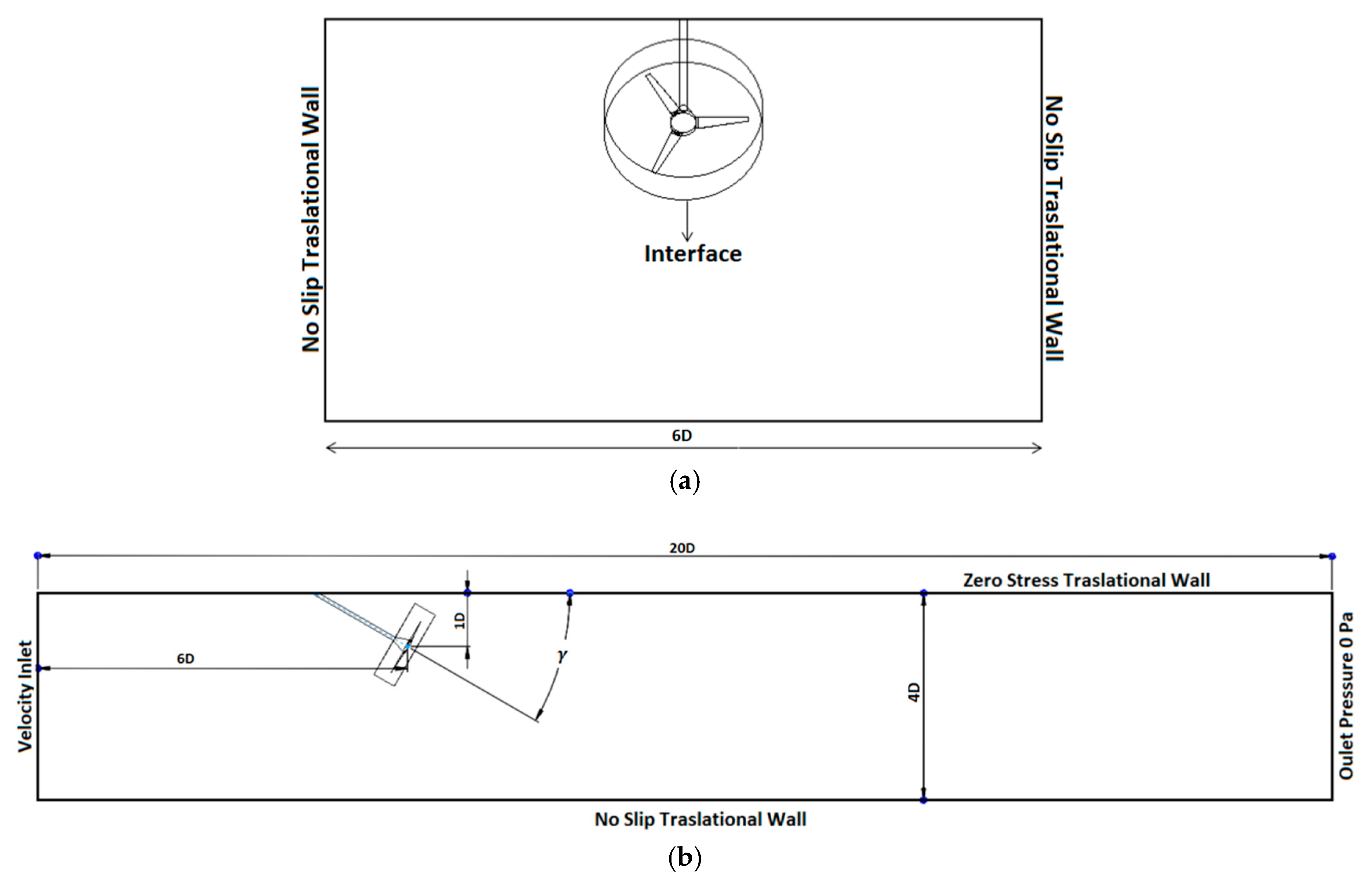
In the present study, three configurations have been analyzed: a first assembly where the rotor is placed perpendicular to the incoming velocity so that the turbine axis is parallel to the flow direction (SP configuration), and two inclined arrangements where the axis makes an angle γ of 15° (SI15 configuration) and 30° (SI30 configuration) regarding the free surface, respectively (see Figure 2b). Obviously, the two last cases mimic the conditions in which the real HAHT operates. The three configurations considered allowing for a quantitative estimation of the influence of the inclination angle on machine performance as well as on the forces acting on the turbine.
The considered computational domain has the following dimensions, which are expressed in terms of the rotor diameter D: length, 20D height, 4D and width, 6D. With such dimensions, the turbine operates in almost isolated conditions, as the resulting blockage ratio is lower than 5%. Moreover, the computational domain is divided into two sub-domains: an inner rotating domain of cylindrical shape, which includes the turbine rotor (blades and hub), and an outer steady domain encompassing the water environment. In the cases of inclined configurations, the shaft was included in this domain, but not in the parallel to flow configuration. To represent the physical rotational motion of the blades, the cylindrical domain rotates with a prescribed angular velocity with respect to the steady domain, which numerically is realized by a sliding mesh technique implemented in the commercial software employed (Fluent v. 14.0, ANSYS, Inc., Canonsburg, PA, USA).
The employed boundary conditions can be appreciated in Figure 2a,b. As indicated in Figure 2b, the left side is specified as a velocity inlet with a constant velocity (equal to 1.0 m/s in this study), the right face is set as a pressure outlet (0 Pa), the bottom boundary (channel bed) consists on a steady non-slip wall) whereas the top border, representing the free surface, was established as a zero stress moving wall translating with the same velocity as that imposed at the inlet. The lateral walls, as shown in Figure 2a, are defined to be non-slip walls. Inside the rotating subdomain is the rotor, this cylinder is connected with the outer domain though interfaces specified as the sliding mesh boundary condition. Moreover, because the turbulence levels at the inlet were not known, it was decided to work with a moderate turbulence intensity equal to 5%.
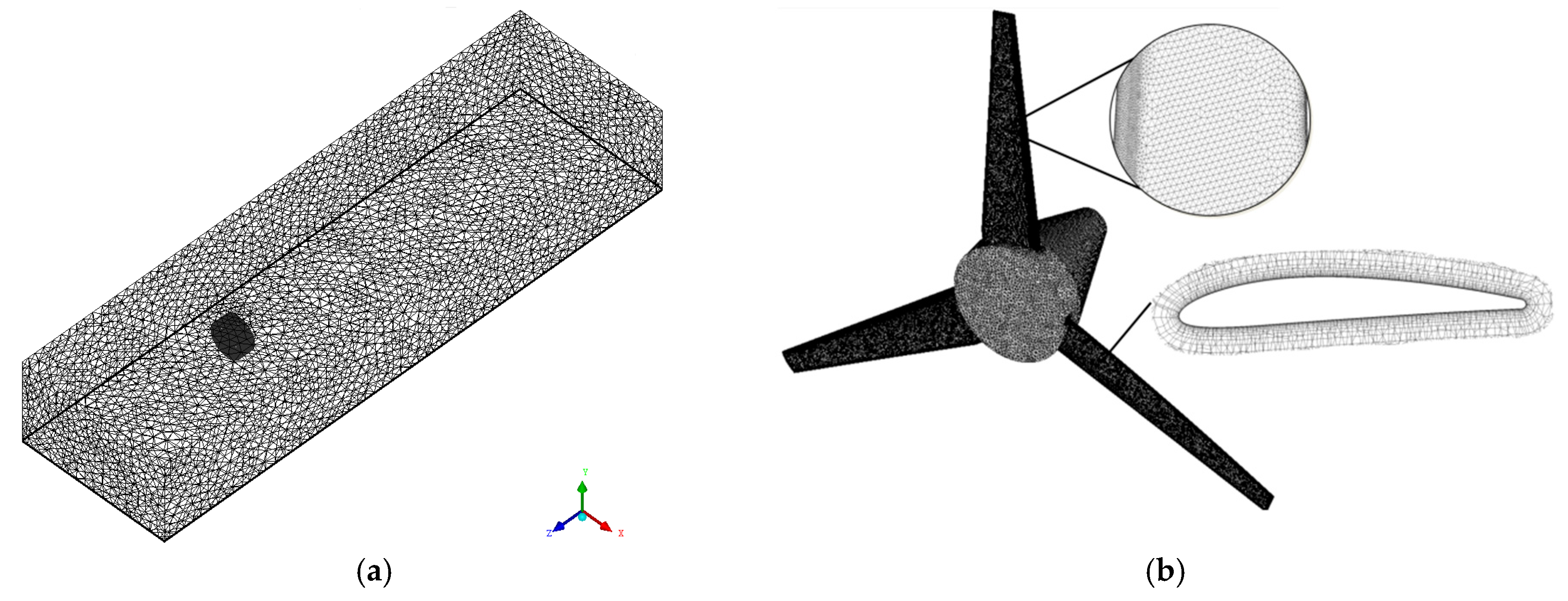
The computational domain has been discretized by means of a non-structured mesh created with the ANSYS ICEM-CFD software (v. 14.0, ANSYS, Inc., Canonsburg, PA, USA). Figure 3a presents a perspective of the employed mesh where the darkest area corresponds to the rotating sub-domain. To adequately describe the boundary layer development, the grid closest to the blades must be fine enough; as an illustration, Figure 3b shows the surface mesh employed in the blades and the hub, which is pretty uniform. Consequently, the mesh around the blade has an O-grid topology with twelve prism layers. Outside the prisms region, a tetras based non-structured grid was constructed, taking care that their aspect ratio is similar to that of the prisms with the purpose of guaranteeing a smooth transition between both mesh regions. Finally, the grid density is higher downstream than upstream the rotor due to the complexity of the flow in the turbine wake. The quality parameters of the meshes have been checked with the tools available in ANSYS ICEM-CFD and are listed in Table 1.
3. Numerical Simulation Methodology
The transient flow around the HAHT was computed with the help of the transient rotor-stator framework, realized by the sliding mesh approach. In that model, the turbine hub and blades rotate counterclockwise (see Figure 4) with a prescribed angular velocity; in this way, the development of the flow field at each time step is described. The interface position between the rotating inner and steady outer sub-domains is actualized every time step allowing for a conservative flux interchange between them. The Shear Stress Transport (SST) model was adopted to describe the turbulent features of the flow. In this study the standard version of such model [21,22] was mainly employed, however, the transition version [23] was also tested. It is well known that the SST model improves the predictions of other two-equation turbulence models in flow configurations where strong adverse pressure gradients occur, such as those happening around a HAHT, and it has been widely used in the simulation of hydraulic turbines [24,25,26,27,28,29,30,31,32,33], where it has become a sort of standard.
Regarding the employed discretization schemes, all the results converged at each time step using second order schemes in space, upwind for the convective and centered for the diffusive terms, respectively, and the second order in time for all the variables. Pressure-velocity coupling is dealt with the SIMPLE (Semi-Implicit Method for Pressure-Linked Equations) approach. Computations were performed for an incident velocity m/s with different angular velocities, depending on the tip speed ratio (see Equation (1) below). The employed time step corresponds to a turbine rotation of around 1°, was chosen after a sensitivity analysis which represents a trade-off between computational cost and accuracy. Moreover, a maximum number of 200 iterations was specified at each time step using a residual convergence criterion of 10−5.
Simulations are started by computing the flow around the HAHT using the steady MFR model of ANSYS-Fluent software (v. 14.0, ANSYS, Inc., Canonsburg, PA, USA), which is used as an initial condition for the transient computation. The unsteady computation is launched, initially using schemes of the first order during approximately ten turbine revolutions to get the flow developed. When the torque has settled down, i.e., the torque curve shows a quasi-periodic behavior, the discretization schemes of the advective terms are changed to second order, firstly for the continuity and momentum equations and later also for the turbulent variables equations. Finally, the simulation was run until the averaged torque difference between two successive turns was below 0.2% [24]. In the present study, for each computed case, at least twenty rotor revolutions have been simulated.
A spatial verification study was performed for the rotor with the shaft parallel to the flow direction (SP configuration). The evaluated operating point was the nominal condition of the wind rotor IT-PE-100 because the same blade design was used for both machines and it corresponds to a tip speed ratio λ = 5.7 (see Equation (1) below) using a rotor angular velocity of 60 rpm. For this grid independence study, the sampled variable was chosen to be the power coefficient CP (see Equation (3) below). According to the usual procedure, three meshes with an increasing number of cells were considered: a coarse grid with elements, an intermediate mesh with , elements and a refined grid with elements. The obtained averaged power coefficients have been the following: 0.2383 (coarse), 0.2430 (intermediate) and 0.2410 (refined). As the difference in is 0.8% between the medium and fine meshes, the intermediate grid was employed in the computations allowing us to maintain an affordable computational time. Based on this result, representing a compromise between the computational cost and accuracy, it was decided to mesh the inclined configurations with a similar distribution and number of elements than the SP case. In those cases, the employed number of elements in the meshes has been elements (SI15 configuration) and elements (SI30 configuration).
The following non-dimensional parameters govern the behavior of the HAHT: the tip speed ratio or TSR () is the non-dimensional angular velocity regarding the incoming velocity, :
where ω is the rotor angular velocity and D its diameter.
The torque coefficient Cm relates to the total torque M, the density of the fluid ρ, and the area swept by the rotor, ; it is written as:
The turbine efficiency, or performance, is expressed by the power coefficient Cp, which is the non-dimensional variable associated with the power produced by the turbine, P:
Cp is obtained as the product of the torque coefficient and the tip speed ratio . Therefore, the operating point of the turbine is defined by the pair .
The total hydrodynamic force acting on each blade is projected on the directions perpendicular to the rotation plane, or normal force , and parallel to it, or tangential force . The tangential force is connected with the torque transmitted by the fluid to the blade while the normal force is responsible for the cyclic loading and fatigue on the blades. In the last case, each blade contribution can be added to compute the normal force acting on the whole rotor—the thrust—which is characterized by the thrust coefficient .
Moreover, on the whole rotor, as an object immersed in a moving fluid, the total hydrodynamic force can be decomposed in a component parallel to the incoming flow velocity, which constitutes the drag, , and in a component in the vertical plane perpendicular to such velocity which constitutes the lift force, . Coefficients associated with such forces are written as:
4. Results
4.1. The Behavior of Non-Dimensional Coefficients Along A Turbine Revolution
In this subsection, the behavior of the power and force coefficients along a cycle is discussed depending on the rotor inclination, and for a TSR . For this operating point, the inflow velocity was and the angular velocity 60 rpm. As indicated previously, the employed turbulence model was k-ω SST [22].
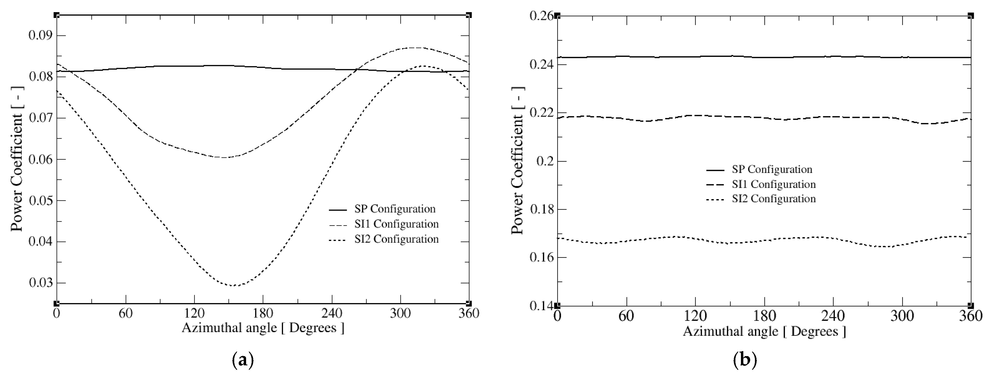
Figure 5 presents the values obtained for the power coefficient in the three considered configurations, SP, SI15 and SI30. This figure illustrates the behavior during a turbine revolution of with the azimuthal angle, defined by Figure 4. Figure 5b shows the contribution of one blade to the power coefficient for the three configurations. In the SP case, the delivered power for one blade depends only very slightly on the azimuthal position, but in the case of the inclined turbines, it shows a clear dependence on such an angle. Therefore, the power coefficient curve consists on a fairly constant curve for SP configuration and on a periodic function with a maximum and a minimum in configurations SI15 and SI30. This fact is associated with differences in the relative velocity experienced by the turbine blades at different angular positions in the inclined turbine cases. As it can be clearly seen in Figure 5b, the oscillation amplitude in increases with the inclination angle (γ), keeping its maximum to very similar values slightly above 0.08 for all cases; however, the minimum value reduces if angle γ increases. Interestingly, the maximum for the SI15 case is slightly higher than the value computed for the SP configuration as it can be appreciated in Figure 5b. Such a maximum value is attained when the blade is around the azimuthal angle of −45° or 315° (see Figure 5b) whilst the minimum is reached around 150°. This fact means that the angular distance between the maximum and minimum is longer (about 195°) than between the minimum and maximum (about 165°), implying that the oscillation behavior is not fully harmonic. The turbine can be observed in Figure 5a: as it is clearly seen, the contributions to the power coefficient of each blade combine to produce a fairly constant value for all the azimuthal positions. Only for the SI30 case can a gentle ripple in the curve be appreciated. Regarding the effect of inclination angle, it was found that in the inclined cases, the power coefficient decreases by 13% (SI15 configuration) and 30% (SI30 configuration) compared to the parallel configuration. It is necessary to mention that the SP configuration presented a small value in the efficiency, around 25%, attributed to the hub geometry, of a truncated cone shape. Such a hub configuration produces a wide wake which increases the drag on the turbine.
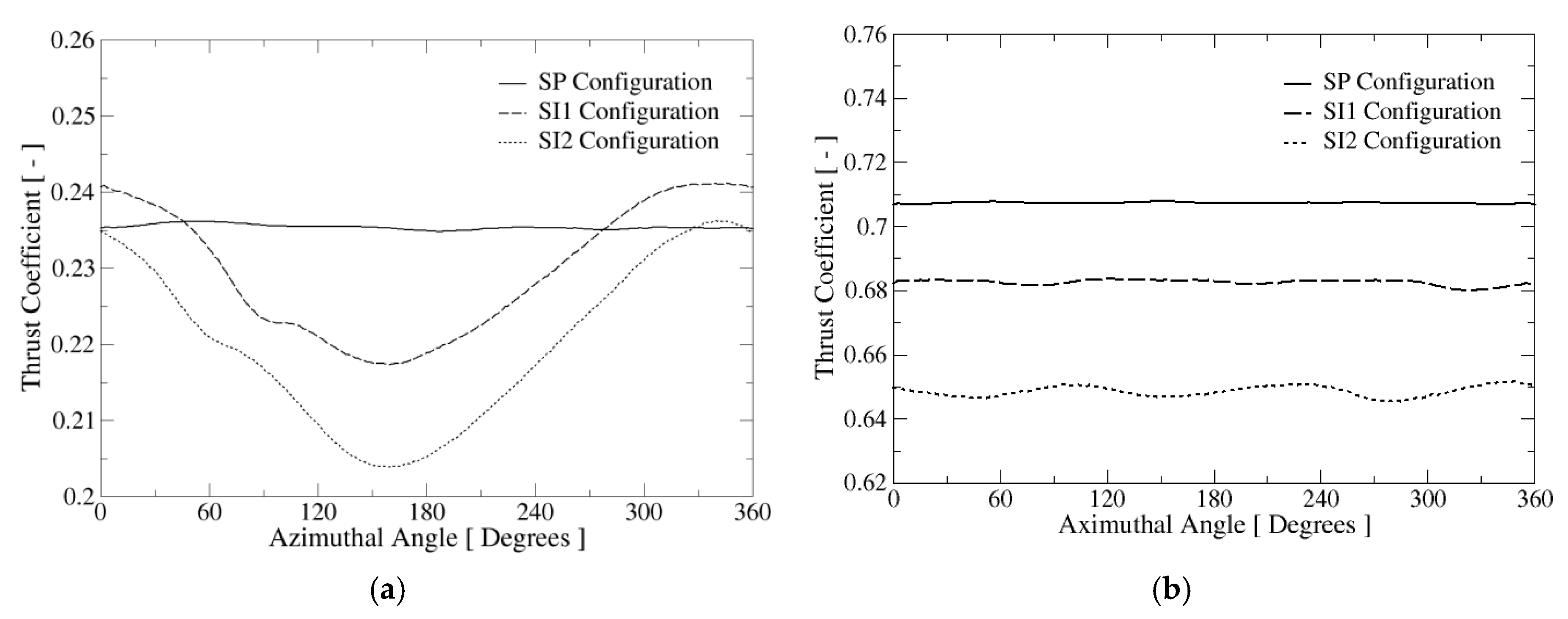
In Figure 6, the behavior of the thrust coefficient (see Equation (4)) versus azimuthal angle along a rotor revolution for one blade (Figure 6b) and the complete turbine (Figure 6a) is illustrated. On the SP configuration, the thrust on each blade is roughly constant along the turn, which also implies that the thrust of the turbine does not vary with the angular position (Figure 6a). However, for the inclined configurations, the normal force on the rotor does vary with the azimuthal angle, which generates alternating loads that could induce material fatigue in the long term. The maximum value of the thrust is experienced by a single blade between the −45° and 0° angles, whereas the minimum appears around 150°. The difference between both thrust values also increases with the inclination angle γ. For instance, in Figure 6b, it can be appreciated that for the SI15, the maximum thrust on the blade overcomes the respective value for the SP turbine. When the total thrust on the turbine is computed (Figure 6a), the inclined configurations experience smaller loads than the SP case, around 4.1% and 10.9% for the SI15 and SI30 cases, respectively. Moreover, the thrust on the turbine is pretty constant along with a revolution for all the cases, showing only a small ripple for an azimuthal angle of 30°.
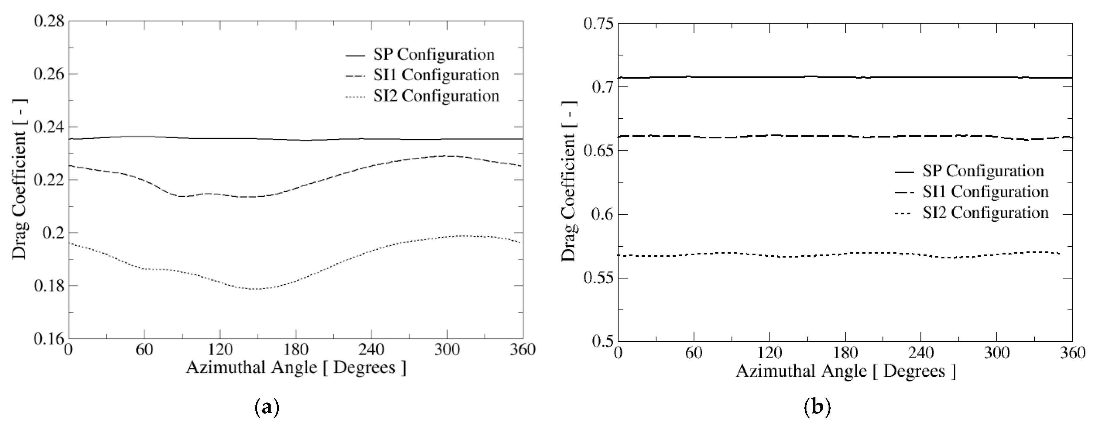
According to Figure 7, as the γ inclination angle increases, the drag coefficient given by Equation (5) decreases. This is true for both the one blade and the full turbine coefficient. Consistent with the previous results, it can be noticed that the inclined cases (SI15 and SI30) present drag coefficients smaller than that of the parallel configuration, around 14% and 20%, respectively. The main reason for that behavior is that, as the inclination angle grows, the rotor transversal area facing the flow decreases, reducing the width of the wake which results in a lower value of the pressure component of the drag force. For the SP configuration, the of one blade keeps a roughly constant value along the whole revolution, but the inclined configurations present a maximum and a minimum. In the SI15 case, two minima of similar values are observed at an azimuthal angle of around 90° and 150°, whereas the maximum is located at around 300°; for the SI30 case, the minimum is placed around 150° and the maximum beyond 310°. Both curves do not show any particular symmetry. For the full turbine, the drag coefficient curves exhibit an approximately constant value with a fairly small ripple for the SI30 configuration.
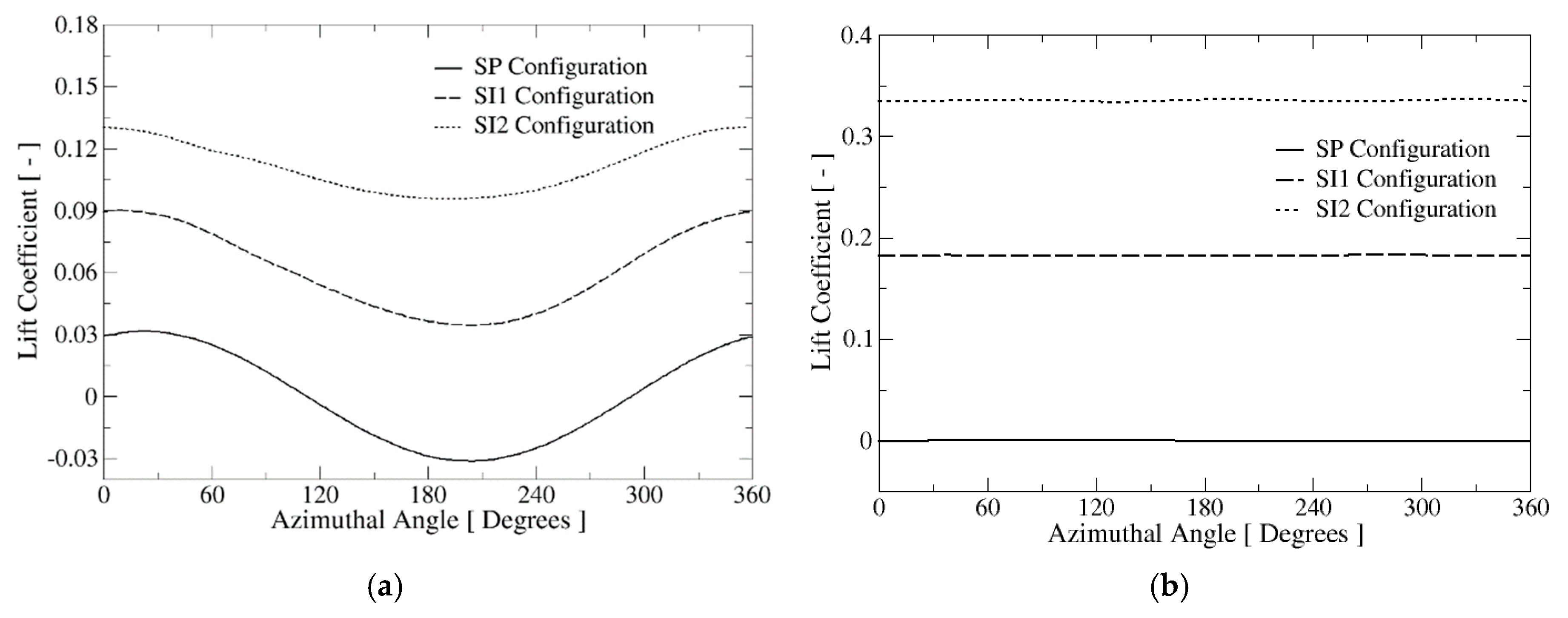
From Figure 8a, it can be noticed that the inclined rotors experience a net upward lift force which is absent in the parallel configuration. The lift coefficient is computed by Equation (5) and in the SP case, each blade experiences a small lift force component which is positive or negative depending on its azimuthal position. In that case, the contributions of the three blades compensate among them to produce a zero net lift coefficient (Figure 8a) for the turbine at each position. This fact is expected, owing to the symmetry of the geometrical configuration. As the inclination angle γ increases, the lift coefficient turns positive and augments with it (Figure 8b). It can be observed that in a cycle, the maximum lift experienced by one blade is located at the azimuthal angle of 0° and the minimum around 210° for the inclined configurations. Again, the contributions to the lift of the three blades compensate providing a fairly constant value of the lift along with a revolution for all the configurations.
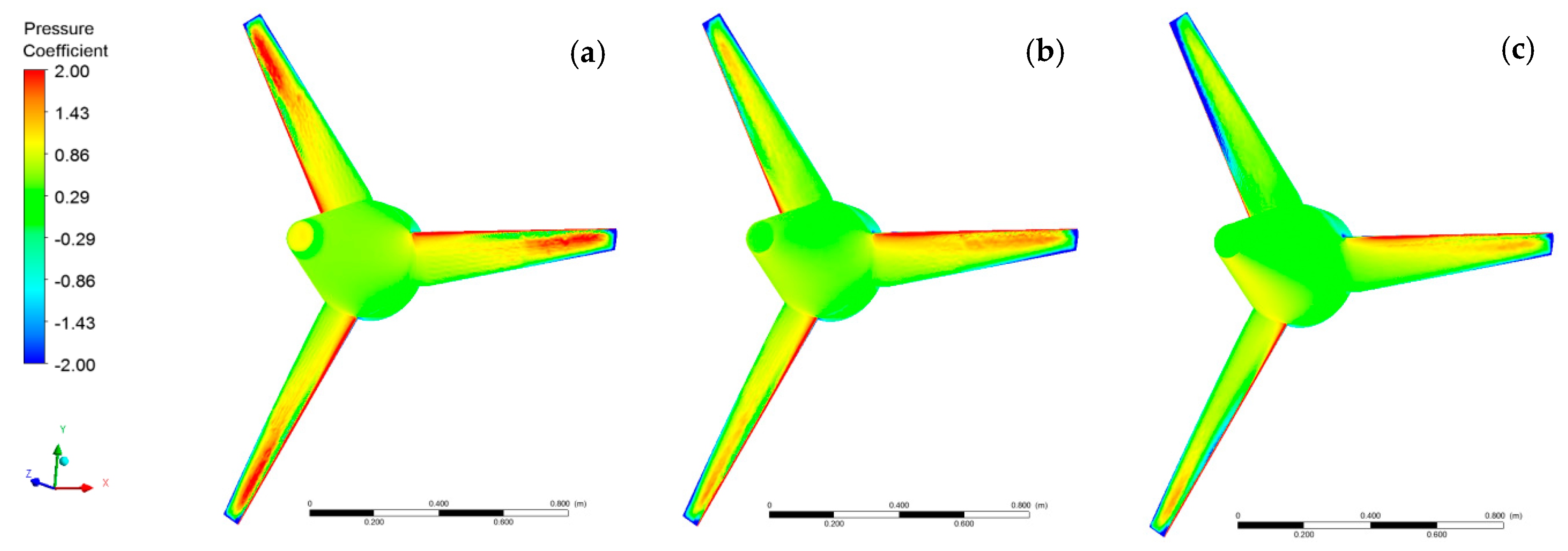
In order to determine the loads on the configurations studied, the total force acting on the rotor was computed. Such a force is smaller for the inclined cases than for the parallel turbine, a fact related with the wider wake in the SP case (which has the effect of increasing the pressure component of the drag force). This fact is illustrated in Figure 9, where the pressure and skin friction coefficients on the blades pressure side are shown. The top row of Figure 9 presents the pressure coefficient for the SP (a), SI1 (b) and SI2 (c) configurations while the bottom row of that figure exhibits the skin friction coefficient for the same configurations: axis parallel (d), inclined 15° (e) and 30° (f) regarding the main flow. From Figure 9a–c it is obvious that pressure acting on the blades decreases with increasing axis inclination; this fact is particularly well observed in the tip of the three blades. Figure 9d–f illustrates the behavior of the skin friction coefficient with inclination angle; in this case, a slight increase of such coefficient is found by increasing the operation slant angle, mainly visible at the blade’s mid-span where a transition between the dark and light blue color is appreciated. However, is the considered cases, the pressure component of the force prevails over the friction component and the net result is that the slanted configurations experience smaller hydrodynamic forces than the SP configuration.
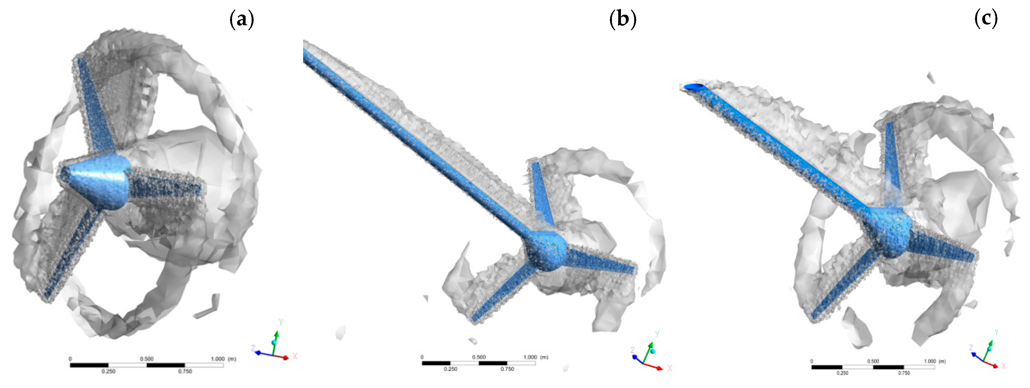
Figure 10 presents a vorticity iso-surface of value 1.5 Hz at the tip speed ratio illustrating the differences in the trailing vortices between the cases of the parallel and inclined turbines. Here, besides the trailing and shed vortices detached from the blades, the wakes generated by the hub and the shaft can also be observed. The hub wake consists on a quasi-steady toroidal vortex that induces a backflow and low pressure in that zone. As a consequence, the drag force, as well as the thrust, is increased on the rotor, reducing the efficiency of the turbine. From Figure 10, it is possible to appreciate that the hub wake in the SP configuration is significantly wider than in the inclined configurations; moreover, the length of the tip vortices is also larger in the SP case.
4.2. Variation of Non-Dimensional Coefficients with the Tip Speed Ratio
In this section, the behavior of the non-dimensional coefficients versus is discussed depending on the turbine inclination. In this case, the inflow velocity is kept constant, equal to , and the turbine angular velocity is varied in the range 40–70 rpm to build the curves.
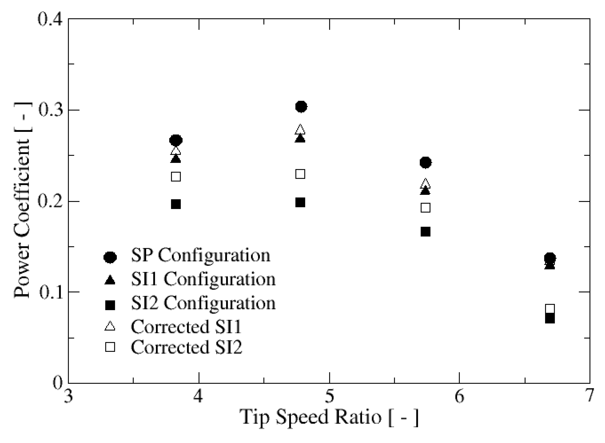
Previously to discuss the performance curve CP-λ, it is necessary to comment that computing the power coefficient using Equation (5) is somehow unfair with the inclined turbine configurations as in such cases the rotor area faced to the incoming flow is reduced by a factor regarding the SP configuration. Because the extracted power is proportional to the area transversal to the flow, it is customary to redefine the power coefficient taking into account this effect. Therefore, a corrected power coefficient,, is defined by Equation (6), where is the power coefficient given by Equation (3):
Figure 11 shows the performance curves for each of the studied configurations. Additionally, for the inclined configurations, the corrected power coefficient is shown in comparison with that computed using Equation (3). As , and the corrected values are closer to the SP values. In all the cases, the maximum of the curve is obtained for with an approximate value of 0.3 for the SP configuration and some consistent lower values for the inclined turbines. For higher values, the angle of attack experienced by the blade is reduced, with the subsequent effect of decreasing the generated lift and the power coefficient. On the other hand, for lower TSR values, the angles of attack of the relative flow approaching the blades increase, eventually overcoming the dynamic stall angles of the profiles, augmenting drag and decreasing lift, which reduces the transmitted torque from the fluid to the blades. Figure 11 demonstrates that the highest performance is obtained for the SP configuration which, regarding to the corrected power coefficient, is on average 6.5% and 25% higher than that for the SI15 and SI30 configurations, respectively.
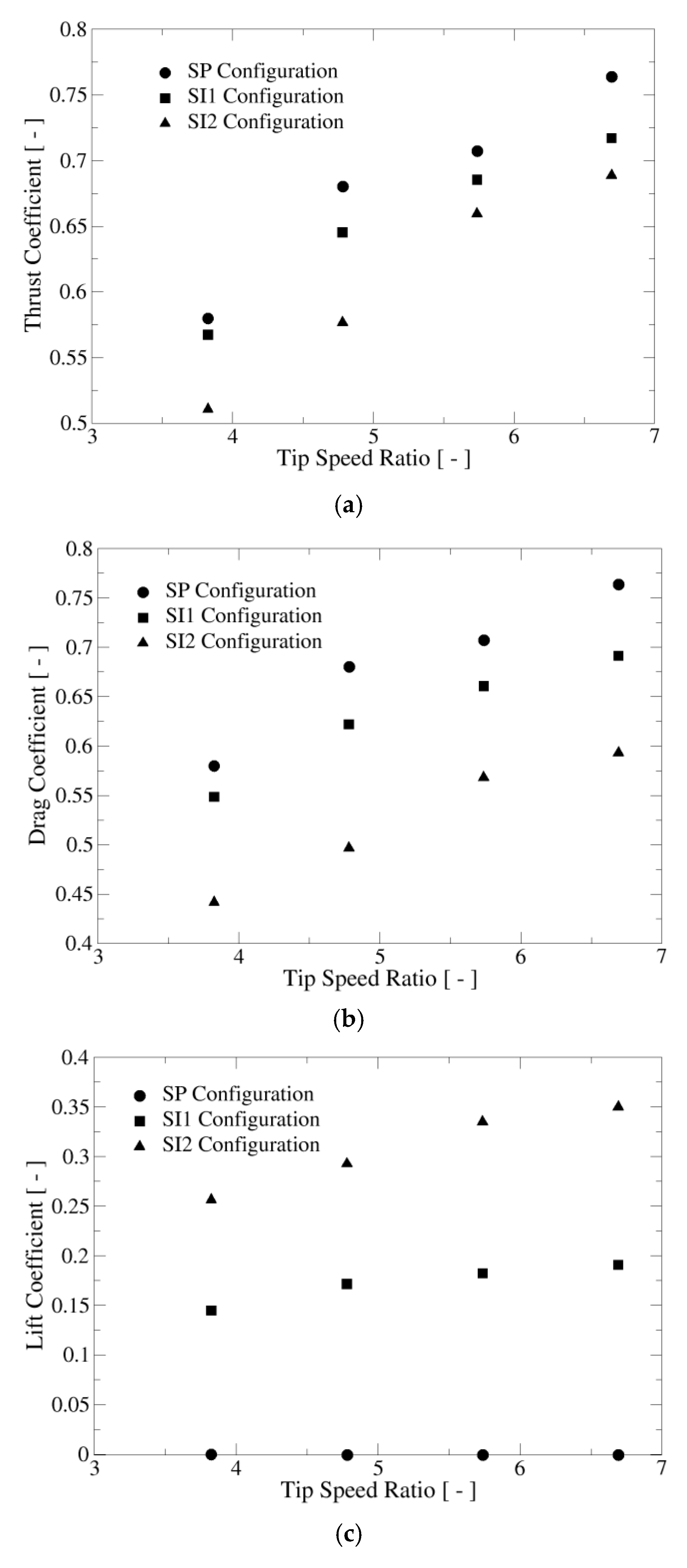
Figure 12 illustrates the behavior of the force coefficients versus tip speed ratio for the three turbine configurations. Figure 12a shows the variation of the thrust coefficient with . It is seen that in all the cases it grows monotonically with the tip speed ratio and, according to the results found previously, it is higher for the SP configuration than for the inclined turbines. As mentioned before, this phenomenon is related to the smaller width of the hub wake for the inclined cases, resulting in a lower pressure drag. However, in spite of the lower thrust, the blades of the inclined turbines are exposed to alternating loads that can induce material fatigue in the long term.
By thinking of the turbine as a whole object immersed in a moving fluid, it is interesting to look to the behavior of the drag and lift forces through its coefficients because such forces have some effects on the turbine operation that should be considered in the design process. Figure 12b presents the variation of the drag coefficient in terms of the tip speed ratio for the studied configurations. In the same way, as happened for the thrust coefficient, the drag coefficient increases monotonically with and decreases with the turbine inclination, approximately 7.5% and 23.2% for the SI15 and SI30 cases, respectively, regarding the SP configuration. Figure 12c shows the change of the lift coefficient with for the three turbine cases. Of course, for the SP configuration, owing to the geometrical symmetry, is very close to zero for all tip speed ratios. For the inclined configurations, on the other hand, it grows monotonically with and also increases with the inclination angle γ. Such a positive lift tends to effectively push up the turbine and eventually could produce vertical oscillations during the turbine’s operation.
Summarizing the results for the performance and force coefficients curves, the inclined configurations have a lower power coefficient than the SP configuration but also experience lower loads. In particular, the rotor drag and thrust decrease with the increasing inclination angle γ and the counterpart of the amplitude of the experienced alternating stresses grows with it. This fact may cause material fatigue in the blades after long periods of operation. Additionally, the fluid forces acting on the blades increase with tip speed ratio for all the studied turbine configurations.
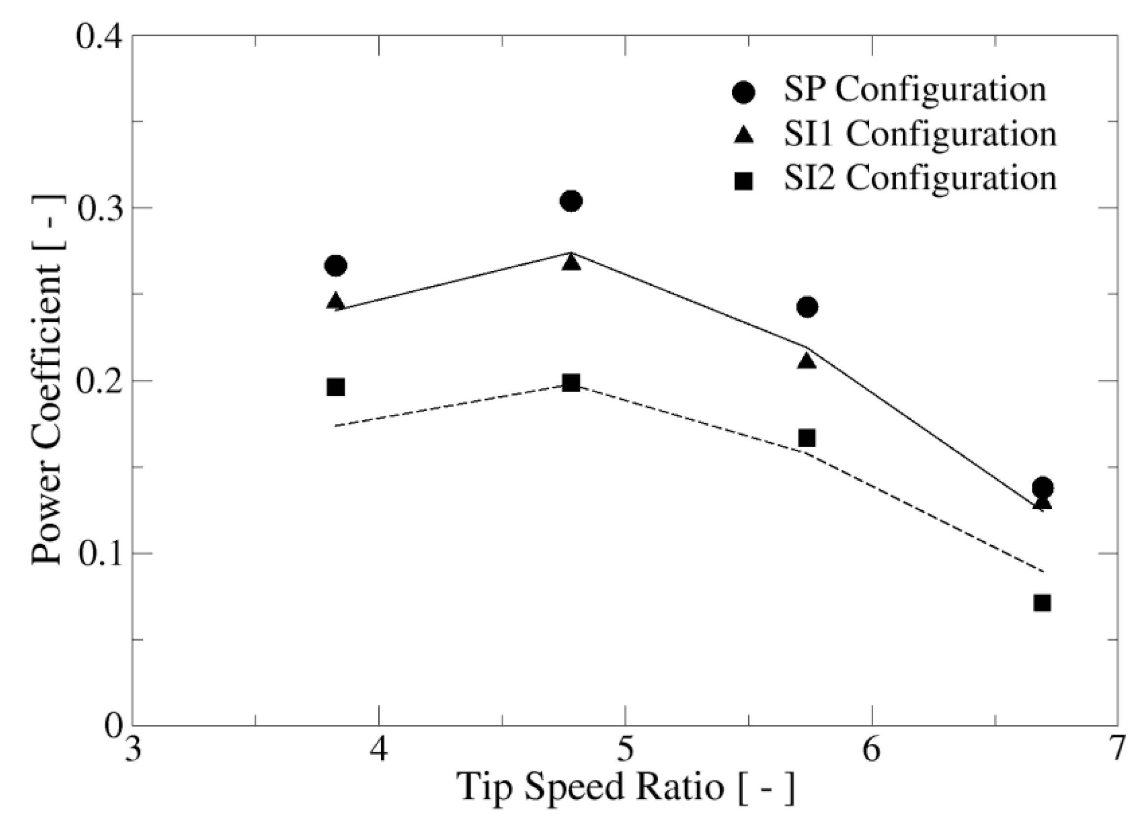
As a final comment, the actuator disc theory can be extended to consider situations where the incident flow makes an angle γ with the direction perpendicular to the rotor [25]. In that case, the maximum power coefficient is given by Equation (7):
Therefore, a common practical approach for estimating the performance of wind turbines when the flow is not perpendicular to the rotor is to multiply the power coefficient by the cube of the cosine of the angle between the incoming velocity and the rotor revolution axis. This procedure is known as the correlation. In this study, the comparison was made using Equation (8), which is an extension of Equation (7) where is the power coefficient obtained for the SP configuration at each considered TSR and is the inclination angle of the rotor. This value was compared with that obtained in the simulation, which is given by Equation (3). See the lines (solid for SI1 and dashed for SI2) in Figure 13.
Figure 13 presents the comparison of applying such a correlation with the CFD results in the inclined configurations. As it can be clearly noticed, for the SI15 case, the correlation works pretty well for the four tip speed ratios computed. In the SI30 case, the two central values for λ are well approximated but for the extreme values, noticeable differences appear: for λ = 3.8 the CFD result is underpredicted by the correlation (about 12%) and for λ = 6.7 it is overpredicted (about 21%). Nevertheless, owing to the simplicity of the correlation, the results are approximate enough from an engineering point of view.
4.3. Comparison of the Results with Transitional Turbulence Modeling
To study the sensitivity of the results to the modeling of the transitional effects on the boundary layer, in addition to the k-ω SST model (SST Standard), the SST Transitional version has been also employed. The Transition SST model includes two additional equations that describe the laminar–turbulent boundary layer transition: the first one for the intermittency factor (the time fraction in which the flow in a point inside the boundary layer is turbulent) and a second equation for the transition momentum thickness Reynolds number [9,26]. The reason behind employing a transition model is that in the hydrokinetic turbine the blade Reynolds number changes along its span and in time, so phenomena such as laminar separation, the transition to turbulence, flow reattachment, and turbulent separation take place in the boundary layer. These phenomena cannot be captured by fully turbulent models, even though the turbulent kinetic energy production could be limited by a damping function.
The performance curve for the SP and SI30 configurations obtained with both turbulence models are shown in Figure 14. For the SP and the SI30 inclined configurations, the average power coefficient estimated with the SST Transition model was incremented regarding the SST standard. The same fact was found previously in the case of vertical axis water turbines [26,27]. However, for the SP turbine, the difference between the predictions of both turbulence models increase as the tip speed ratio grows and, for the largest value considered (λ = 6.7), it is about 40%. This behavior was found previously by Reference [27] in a vertical axis tidal turbine with even larger differences in the values obtained with both turbulence models. For the SP2 configuration, on the other hand, the differences in predictions between both turbulent models decrease as the tip speed ratio increases, with the highest difference being about 15% obtained for λ = 3.8.
Although not shown, the behavior of the force coefficients with the turbulence model is similar to that of the power coefficients: the transitional version provides higher values than the standard SST. Therefore, it can be concluded that the transitional formulation predicts that the transfer of energy from the fluid to the blades is improved regarding the standard formulation, at least in the range of TSRs considered in the present study.
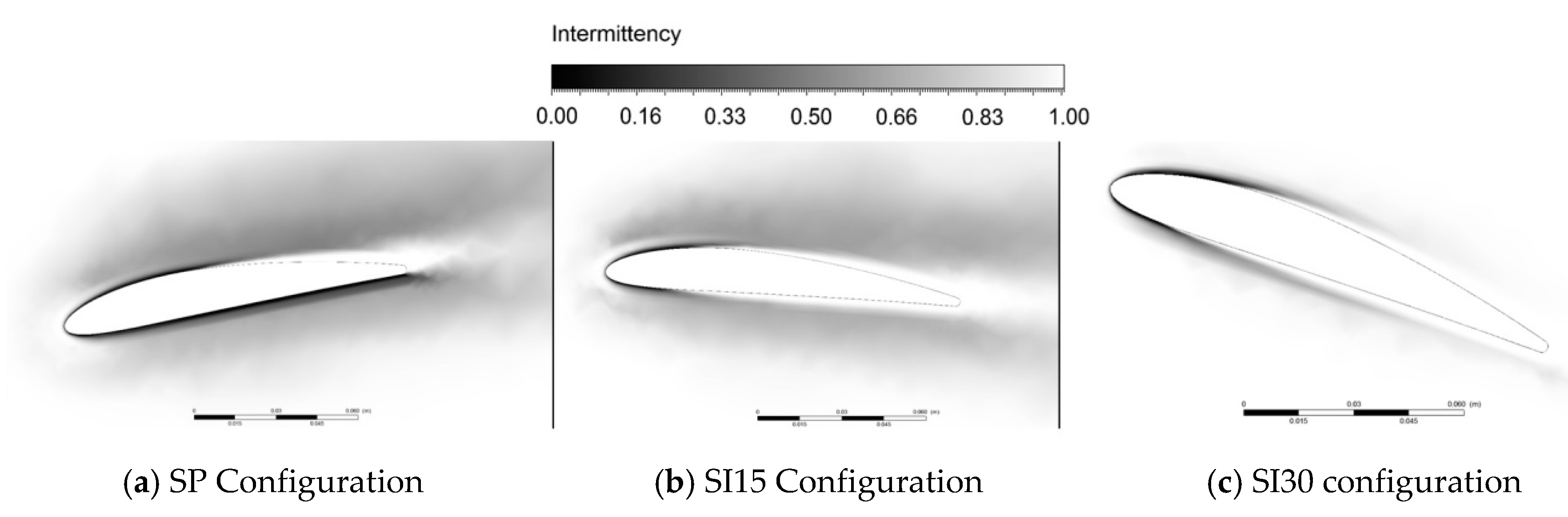
As an example to highlight the transitional behavior of the boundary layer computed with the SST Transition turbulence model, Figure 15 shows the intermittency contours on a section of the first blade (at mid-span) in the SP, SI15 and SI30 configurations at the 0° azimuthal position. In Figure 15, values close to zero (black color) indicate the laminar regime whereas values close to 1 (white color) indicate the mean turbulent boundary layer. In the contour plots flow proceeds from bottom to top. As it is readily observed, the contour plots present noticeable differences. In the SP configuration (Figure 15a), the intrados boundary layer develops entirely in the laminar regime, while in the extrados layer, laminar-turbulent transition phenomena happen (the contours evolve from black to white along the extrados surface); besides, around the profile, a laminar flow envelope is clearly visible (variable grey intensity). Such an envelope is also present around the profile for the SI15 configuration (Figure 15b), but here the boundary layer experiences laminar to turbulent transition in both surfaces (intrados and extrados). However, for the SI30 configuration (Figure 15c), such a laminar flow envelope disappears, being turbulent for the major part of the flow around the profile; also, the transition between laminar and turbulent regimes is very clear for intrados and extrados. Finally, although not shown, such transitional behavior changes along the blade span, a fact that illustrates the water flow complexity in the vicinity of the turbine blades of the HAHT.
5. Comparison of CFD Simulations with Other Sources
As previously commented; the evaluated turbine was empirically designed and tested in situ only for feasibility purposes, on the Cauca river in the southwest of Colombia. However, the prototype was never adequately experimentally characterized. Therefore, data on the extracted power in terms of incident flow velocity or turbine angular velocity are not available. Consequently, some alternative for comparing the obtained CFD results have to be devised.
As a first step, the CFD computations have to be validated versus the experimental results in the HAHT configuration. For that purpose, the experimental measurements reported in Reference [34] have been considered. Such experiments have been employed by several authors to validate different types of numerical computations, from BEM to CFD [11,34]; therefore, they constitute an appropriate source for validating the CFD computations. In the experiments of Reference [34], the model turbine rotor is placed perpendicularly to the main flow direction, so its inclination angle γ is zero; the rotor diameter was 800 mm with blades based on the profile NACA 63-8XX. The considered experiments for comparison are those corresponding to a pitch set angle of 0° and with an inflow velocity of 1.4 m/s.
The additional CFD simulations consider a grid arrangement similar to that of the case of the inclined rotor: the computational domain has the same dimensions as those shown in Figure 2. The boundary conditions are also the same and the grid size is similar to that employed for the Aquavatio model comprising around eight million elements, also using 12 prisms layers to resolve the flow in the boundary layer. Three tip speed ratios close to the point of the maximum efficiency have been simulated. The obtained results for the power coefficient are presented in Figure 16. In that figure, the crosses correspond to the experimental points and some other numerical simulations are also included for the purpose of comparison: the results of the commercial software GH-tidal (based on BEM) presented by Bahaj et al. [34] and the CFD results of Wu et al. [11]. Regarding the experimental data, the BEM results slightly over-predict them, while the CFD predictions of Reference [11] (based on the standard k-ε turbulence model) are below the experiments, except for λ = 6. The present CFD computations based on the SST model of turbulence, provide values that are fairly close to the measurements, at least in the three computed TSR, a fact that is attributed to the better performance of the SST model regarding the k-ε model in these kinds of rotating machines [27]. The results presented in Figure 15 show that the employed CFD simulations are appropriate enough to be used in the computations of HAHTs. References [35,36,37] present additional examples in other Engineering applications where CFD techniques have been found to perform adequately.
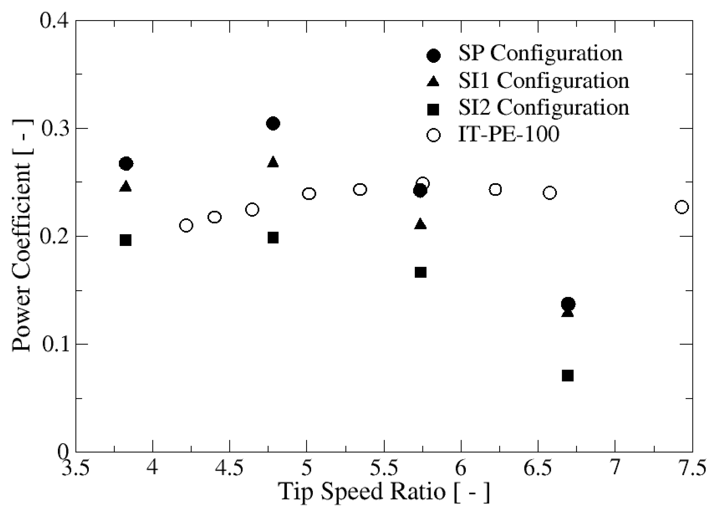
Another option to compare the results obtained in this work is provided by the wind turbine IT-PE-100 developed by the company ITDG [20,28] because the blade design was adopted by the computed hydrokinetic turbine Aquavatio. However, the hub design is very different in both machines; in the river turbine, the hub has a shape of a truncated cone (see Figure 1a) motivated for structural reasons. This hub geometry, as already shown in Figure 10, generates a wide wake that affects the performance of the turbine.
The experimental power-velocity curve of the wind rotor IT-PE-100 is available [28]. Nominal values of incident velocity and angular velocity are 6.5 m/s and 420 rpm, respectively, giving a nominal tip speed ratio of λ = 5.75, for the nominal diameter of 1.7 m; this TSR is very close to the value considered initially in this work for the hydrokinetic turbine, λ = 5.7. With the previous data, the performance curve for turbine IT-PE-100 can be constructed. vs. λ curves for both turbines are shown in Figure 17. It can be seen that the performance of both is roughly the same for λ = 5.75, which is around 25% (SP configuration). The wind turbine presents a fairly flat curve for the considered range of tip speed ratios, while the hydrokinetic turbine presents a clear maximum at λ = 4.8 and decreasing for larger and lower values, as discussed in Section 4.2. In Figure 17, the performance curves for the inclined turbines are also included just for comparison. From that figure, it can be seen that, for the SP configuration, the efficiency curve is displaced towards lower values of λ than that of the IT-PE-100 rotor, which is obviously a consequence of the different operating conditions. However, the maximum of both turbines is totally comparable, about 25–30%. Therefore, although the working conditions of both machines differ, their performance curves are similar because they share the blade design and have very similar dimensions.
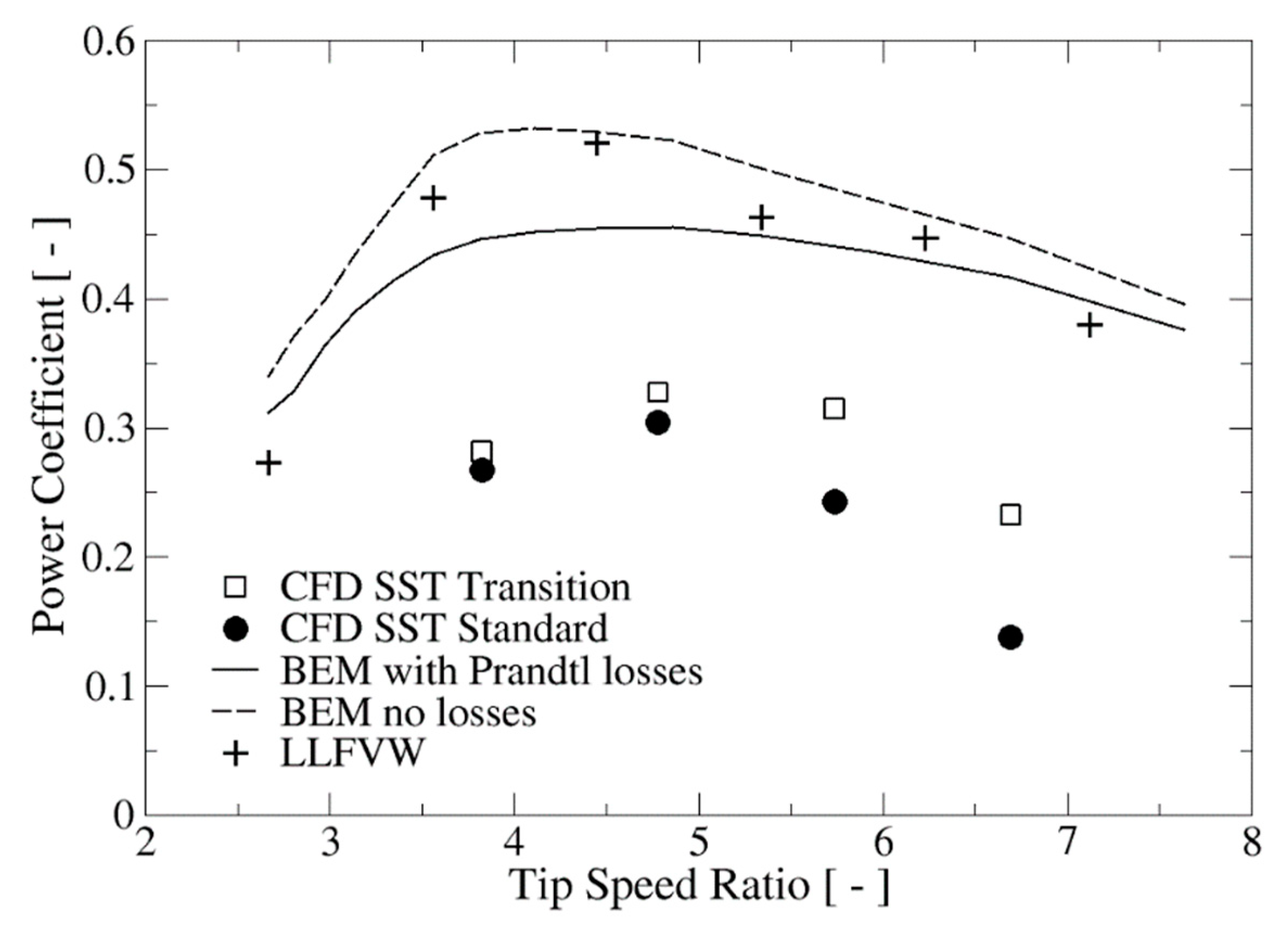
The third comparison was carried out versus the results provided by the Qblade software [29] which is available online at www.q-blade.org. Qblade is a general purpose software for wind turbine evaluation, horizontal and vertical. It employs well established simplified methods such as the BEM (Blade Element Momentum) model and other vortex based models such as LLFVW (Lifting Line Free Vortex Wake) and includes extra features such as structural and aeroelastic modules. In spite of Qblade being developed for wind turbines, it allows us to modify the physical properties of the working fluid so it is applicable to evaluate hydrokinetic turbines. Here, the results obtained by the BEM and LLFVW methods are compared with the CFD results for the SP configuration in Figure 18.
From Figure 18 it is obvious that the simplified models provide substantially higher power coefficients than those obtained with CFD. This assertion is true for both methods, BEM and LLFVW, even including the Prandtl tip and root losses. It is interesting to remark that the LLFVW method, which is one of the most sophisticated techniques among the simplified approaches, provides results very close to those of the BEM. The differences between such predictions and those obtained with CFD can be explained as follows: on the one hand, it is known that BEM tends to overestimate the power coefficient, specifically for high solidity turbines and, on the other hand, in the simplified methods the hub is not taken into account in the computation. It has been already remarked that the truncated cone shape of the hub produces a broad wake responsible for augmenting the thrust and drag forces on the rotor, consequently reducing the turbine performance.
Additionally, as a reference, Figure 18 includes the results computed with the SST Transition turbulence model, which are also well below the simplified method’s predictions.
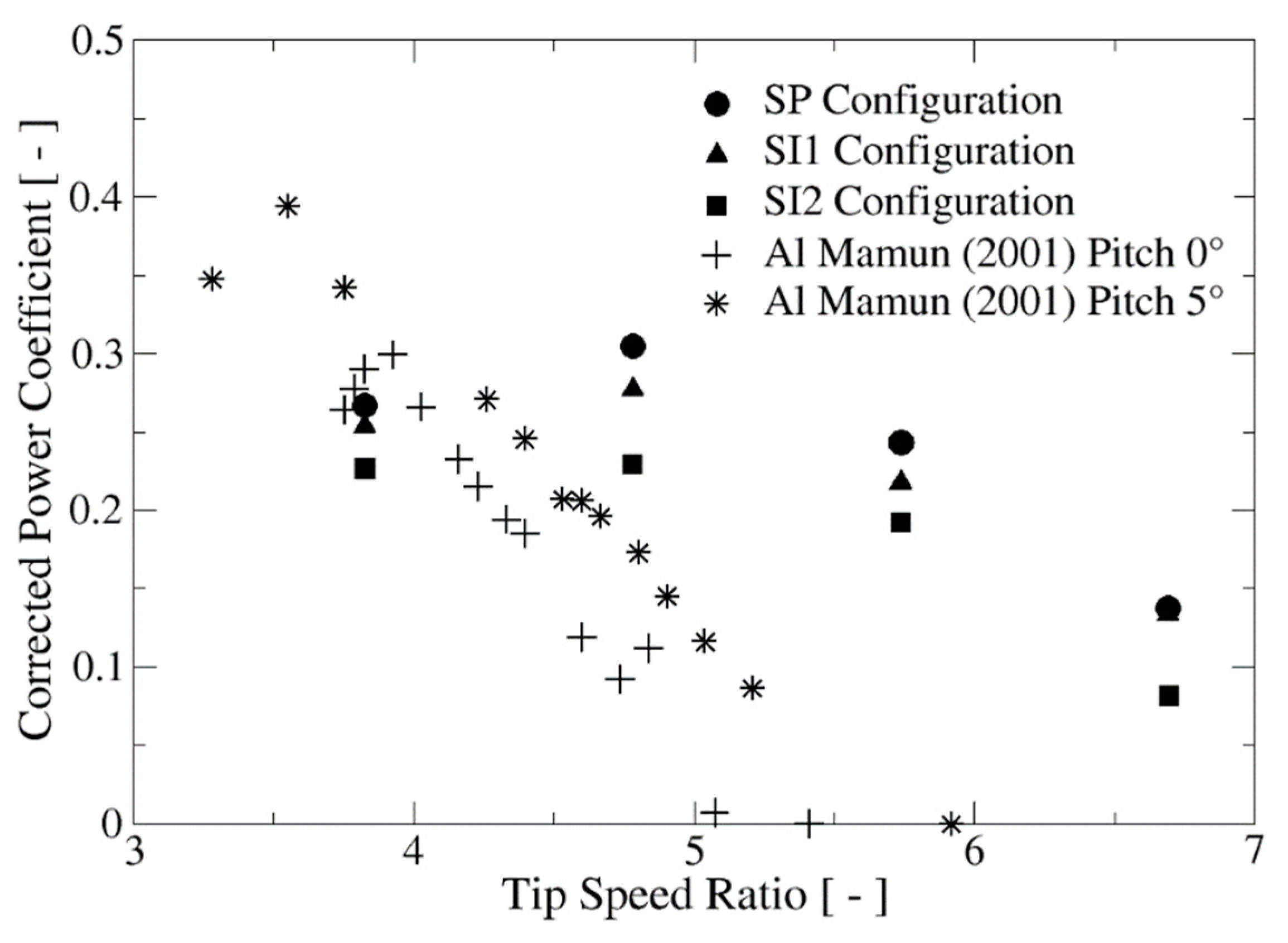
As a final comparison, the experimental results of Reference [18] have been considered. Al Mamun [18] conducted an experimental study of the performance of a small three-bladed hydrokinetic turbine in a water channel working with an inclination angle γ = 45. The rotor diameter was small, 0.223 m, and the blade was based on the NACA 4412 profile. The rotation angular velocity was about 120 rpm. The experimental results are summarized in Appendix G of Reference [18] and those corresponding to an incident velocity of 0.65 m/s are presented in Figure 19 compared with the CFD computations of the present study.
Although the tip speed ratio ranges between both turbines are different, the maximum values of the power coefficient are comparable for the pitch angle of 0 (see Figure 19). For λ < 4, the experimental power coefficient of Reference [18] dropped drastically, so the range of TSRs for which the turbine was able to produce power is much reduced than for the turbine simulated in this work. Al Mamun [18] found that when the blade was installed with a pitch angle of 5°, increased for the particular value of the employed incident velocity. Moreover, if the incoming flow speed was also reduced, the maximum value of decreased and it was displaced toward lower values of the tip speed ratio.
In summary, although a proper validation of the performed CFD simulations has not been possible due to the absence of experimental measurements in the HAHT studied, comparisons with experimental measurements in similar systems and with the results provided by more simplified methods indicate that the obtained numerical results are consistent and plausible. They provide the expected trends for the influence of turbine inclination on its performance, allowing us to quantitatively estimate the reduction of efficiency and thrust coefficient on the rotor when its operation slant angle increases.
6. Conclusions
This contribution addresses for the first time, to the best of authors’ knowledge, the numerical CFD computation of a Garman type horizontal axis hydrokinetic turbine operating with its shaft inclined regarding the main stream direction. The performed CFD simulations have been unsteady and three-dimensional, describing the transient features of the water flow around the blades. The turbulent dynamics of the flow was dealt with the Shear Stress Transport (SST) turbulence model, where the boundary layer laminar-to-turbulent transitional effects have also been included. The computational results allowed us to quantitatively estimate the efficiency reduction in the inclined configurations regarding the SP configuration as about 6.5% for SI15 and 25% for SI30. The computed efficiency curves (power coefficient versus tip speed ratio) for the inclined configurations were compared with those provided with the so-called correlation; as a result, the correlation sufficiently approximates the CFD results for tip speed ratios close to the maximum efficiency point, although it presents noticeably differences for values of outside of this range. Additionally, it has been found that the rotor in the inclined configurations experiences lower drag and thrust forces than in the SP case, which is due to the reduced wake width in the formers, a fact that has the effect of decreasing the pressure component of the drag. Nevertheless, although the net forces acting on the rotor are smaller in the SI15 and SI30 configurations than in the SP arrangement, in those cases the blades are exposed to cyclic stresses that might lead to failure due to fatigue after long periods of operation. When the modeling of the laminar-to-turbulent transition boundary layer is considered, by means of the SST Transition turbulence model, a slight increase of the estimated power coefficients is obtained, a fact found previously in other works dealing with vertical axis water turbines [26,27], implying a higher energy transmission from the water to the rotor in such conditions. Finally, the computed results have been compared with experimental measurements in similar systems and with those obtained with more simplified approaches, which allows us to conclude that the expected trends of the influence of shaft inclination on turbine performance have been adequately estimated by the present simulations. In the near future, we plan to estimate the effect of the alternating stresses appearing in the inclined configurations on the fatigue behavior of the turbine and its lifetime. Moreover, we intend to numerically study the free surface effects on turbine performance through the coupling of the transient rotor-stator technique with the volume of fluid method.
Author Contributions
Conceptualization, O.D.L. and S.L.; Data curation, L.T.C.; Formal analysis, O.D.L. and S.L.; Funding acquisition, S.L. and O.D.L.; Investigation, L.T.C.; Methodology, O.D.L. and S.L.; Resources, S.L.; Supervision, O.D.L. and S.L.; Validation, L.T.C.; Visualization, L.T.C.; Writing—review & editing, S.L.
Funding
This research was partially funded by the Young Researchers program from the Colombian administrative department of science, technology and innovation, Colciencias (Grant number 0001635894) and partially by the Dirección de Investigaciones y Desarrollo Tecnológico of Universidad Autónoma de Occidente and Vicerrectoria de Investigaciones of Universidad de los Andes (Grant number 16Inter-265). The APC was funded by Universidad Autónoma de Occidente.
Conflicts of Interest
The authors declare no conflict of interest.
References
- Silva, P.A.S.F. Estudo Numérico de Turbinas Hidrocinéticas de Eixo Horizontal. Master’s Thesis, University of Brasilia, Brasília, Brazil, 2014. [Google Scholar]
- Khan, M.J.; Iqbal, M.T.; Quaicoe, J.E. River current energy conversion systems: Progress, prospects and challenges. Renew. Sustain. Energy Rev. 2008, 12, 2177–2193. [Google Scholar] [CrossRef]
- Güney, M.S.; Kaygusuz, K. Hydrokinetic energy conversion systems: A technology status review. Renew. Sustain. Energy Rev. 2010, 14, 2996–3004. [Google Scholar] [CrossRef]
- Muratoglu, A.; Yuce, M.I. Design of a river hydrokinetic turbine using optimization and CFD Simulations. J. Energy Eng. 2017, 143. [Google Scholar] [CrossRef]
- Gaden, D.L. An Investigation of River Kinetic Turbines: Performance Enhancements, Turbine Modeling Techniques, and an Assessment of Turbulence Models. Ph.D. Thesis, University of Manitoba, Winnipeg, MB, Canada, 2007. [Google Scholar]
- Guney, M.S. Evaluation and measures to increase performance coefficient of hydrokinetic turbines. Renew. Sustain. Energy Rev. 2011, 15, 3669–3675. [Google Scholar] [CrossRef]
- Bai, G.; Li, J.; Fan, P.; Li, G. Numerical investigations of the effects of different arrays on power extractions of horizontal axis tidal current turbines. Renew. Energy 2013, 53, 180–186. [Google Scholar] [CrossRef]
- Van Els, R.H.; Junior, A.C.P.B. The Brazilian experience with hydrokinetic turbines. Energy Procedia 2015, 75, 259–264. [Google Scholar] [CrossRef]
- López, O.; Meneses, D.; Quintero, B.; Laín, S. Computational study of transient flow around Darrieus type cross flow water turbines. J. Renew. Sustain. Energy 2016, 8, 014501. [Google Scholar] [CrossRef]
- Kang, S.; Borazjani, I.; Colby, J.A.; Sotiropoulos, F. Numerical simulation of 3D flow past a real-life marine hydrokinetic turbine. Adv. Water Resour. 2012, 39, 33–43. [Google Scholar] [CrossRef]
- Wu, H.; Chen, L.; Yu, M.; Li, W.; Chen, B. On design and performance prediction of the horizontal axis water turbine. Ocean Eng. 2012, 50, 23–30. [Google Scholar] [CrossRef]
- Guo, Q.; Zhou, L.J.; Xiao, Y.X.; Wang, Z.W. Flow field characteristics analysis of a horizontal axis marine current turbine by large eddy simulation. IOP Conf. Ser. Mater. Sci. Eng. 2013, 52, 052017. [Google Scholar] [CrossRef] [Green Version]
- Malki, R.; Williams, A.J.; Croft, T.N.; Togneri, M.; Masters, I. A coupled blade element momentum—Computational fluid dynamics model for evaluating tidal stream turbine performance. Appl. Math. Model. 2013, 37, 3006–3020. [Google Scholar] [CrossRef]
- Guo, Q.; Zhou, L.; Wang, Z. Comparison of BEM-CFD and full rotor geometry simulations for the performance and flow field of a marine current turbine. Renew. Energy 2015, 75, 640–648. [Google Scholar] [CrossRef]
- Masters, I.; Williams, A.T.; Croft, N.; Michael, T.; Edmunds, M.; Zangiabadi, E.; Fairley, L.; Karunarathna, H. A Comparison of numerical modelling techniques for tidal stream turbine analysis. Energies 2015, 8, 7833–7853. [Google Scholar] [CrossRef]
- Zhang, Y.; Zhang, J.; Zheng, Y.; Yang, C.; Zang, W.; Fernandez-Rodriguez, E. Experimental analysis and evaluation of the numerical prediction of wake characteristics of tidal stream turbine. Energies 2017, 10, 2057. [Google Scholar] [CrossRef]
- Lee, J.H.; Park, S.; Kim, D.H.; Rhee, S.H.; Kim, M.C. Computational methods for performance analysis of horizontal axis tidal stream turbines. Appl. Energy 2012, 98, 512–523. [Google Scholar] [CrossRef]
- Al Mamun, N.H. Utilization of River Current for Small Scale Electricity Generation in Bangladesh. Master’s Thesis, University of Bangladesh, Dhaka, Bangladesh, 2001. [Google Scholar]
- Islam, A.S.; Al-Mamun, N.H.; Islam, M.Q.; Infield, D.G. Energy from river current for small scale electricity generation in Bangladesh. In Proceedings of the Conference C76 of the Solar Energy Society, Belfast, UK, 10–11 September 2001; pp. 207–213. [Google Scholar]
- Chiroque, J.; Dávila, C. Microaerogenerador IT-PE-100 Para Electrificación Rural; Soluciones Prácticas-ITDG: Lima, Perú, 2012. (In Spanish) [Google Scholar]
- Menter, F.R. Zonal two equation k-turbulence models for aerodynamic flows. In Proceedings of the 23rd Fluid Dynamics, Plasmadynamics, and Lasers Conference, Orlando, FL, USA, 6–9 July 1993. [Google Scholar] [CrossRef]
- Menter, F.R. Two-equation eddy-viscosity turbulence models for engineering applications. AIAA J. 1994, 32, 269–289. [Google Scholar] [CrossRef]
- Langtry, R.B.; Menter, F.R. Correlation-based transition modeling for unstructured parallelized computational fluid dynamics codes. AIAA J. 2009, 47, 2894–2906. [Google Scholar] [CrossRef]
- Balduzzi, F.; Bianchini, A.; Malece, R.; Ferrara, G.; Ferrari, L. Critical issues in the CFD simulation of Darrieus wind turbines. Renew. Energy 2016, 85, 419–435. [Google Scholar] [CrossRef]
- Burton, T.; Sharpe, D.; Jenkins, N.; Bossanyi, E. Wind Energy Handbook; John Wiley & Sons, Ltd.: New York, NY, USA, 2001. [Google Scholar]
- Laín, S.; Taborda, M.A.; López, O.D. Numerical study of the effect of winglets on the performance of a straight blade Darrieus water turbine. Energies 2018, 11, 297. [Google Scholar] [CrossRef]
- Marsh, P.; Ranmuthugala, D.; Penesis, I.; Thomas, G. The influence of turbulence model and two and three-dimensional domain selection on the simulated performance characteristics of vertical axis tidal turbines. Renew. Energy 2017, 105, 106–116. [Google Scholar] [CrossRef] [Green Version]
- Chiroque, J.; Sánchez, T.; Dávila, C. Microaerogeneradores de 100 y 500 W-Modelos IT-PE-100 y SP-500; Soluciones Prácticas-ITDG: Lima, Perú, 2008. (In Spanish) [Google Scholar]
- Marten, D.; Wendler, J.; Pechlivanoglou, G.; Nayeri, C.N.; Paschereit, C.O. Qblade: An open source tool for design and simulation of horizontal and vertical axis wind turbines. Int. J. Emerg. Technol. Adv. Eng. 2013, 3, 264–269. [Google Scholar]
- Mukherji, S.S. Design and Critical Performance Evaluation of Horizontal Axis Hydrokinetic Turbines. Master’s Thesis, Missouri University of Science and Technology, Rolla, MO, USA, 2010. [Google Scholar]
- Kolekar, N.; Hu, Z.; Banerjee, A.; Du, X. Hydrodynamic design and optimization of hydro-kinetic turbines using a robust design method. In Proceedings of the 1st Marine Energy Technology Symposium (METS13), Washington, WA, USA, 10–11 April 2013. [Google Scholar]
- Harrison, M.E.; Batten, W.M.J.; Myers, L.E.; Bahaj, A.S. Comparison between CFD simulations and experiments for predicting the far wake of horizontal axis tidal turbines. IET Renew. Power Gener. 2010, 4, 613–627. [Google Scholar] [CrossRef]
- Suatean, B.; Colidiuc, A.; Galetuse, S. CFD methods for wind turbines. In Proceedings of the 9th International Conference on Mathematical Problems in Engineering, Aerospace and Sciences: ICNPAA, Vienna, Austria, 10–14 July 2012; pp. 998–1002. [Google Scholar]
- Bahaj, A.S.; Batten, W.M.J.; McCann, G. Experimental verifications of numerical predictions for the hydrodynamic performance of horizontal axis marine current turbines. Renew. Energy 2007, 32, 2479–2490. [Google Scholar] [CrossRef]
- Sommerfeld, M.; Laín, S. From elementary processes to the numerical prediction of industrial particle-laden flows. Multiph. Sci. Technol. 2009, 21, 123–140. [Google Scholar] [CrossRef]
- Laín, S.; García, M.; Quintero, B.; Orrego, S. CFD numerical simulations of Francis turbines. Rev. Fac. Ing. Univ. Antioq. 2010, 51, 24–33. [Google Scholar]
- Caballero, A.D.; Laín, S. Numerical simulation of non-Newtonian blood flow dynamics in human thoracic aorta. Comput. Methods Biomech. Biomed. Eng. 2015, 18, 1200–1216. [Google Scholar] [CrossRef] [PubMed]
Figure 1.
The schematics of the inclined hydrokinetic turbine showing its components (a) and isometric view of the geometrical model (b).
Figure 1.
The schematics of the inclined hydrokinetic turbine showing its components (a) and isometric view of the geometrical model (b).

Figure 2.
The front view (a) and side view (b) of the geometry for the inclined HAHT. The employed boundary conditions are also shown.
Figure 2.
The front view (a) and side view (b) of the geometry for the inclined HAHT. The employed boundary conditions are also shown.

Figure 3.
The overview of the mesh used at the steady domain (a) and the surface mesh on the turbine blades and hub (b).
Figure 3.
The overview of the mesh used at the steady domain (a) and the surface mesh on the turbine blades and hub (b).

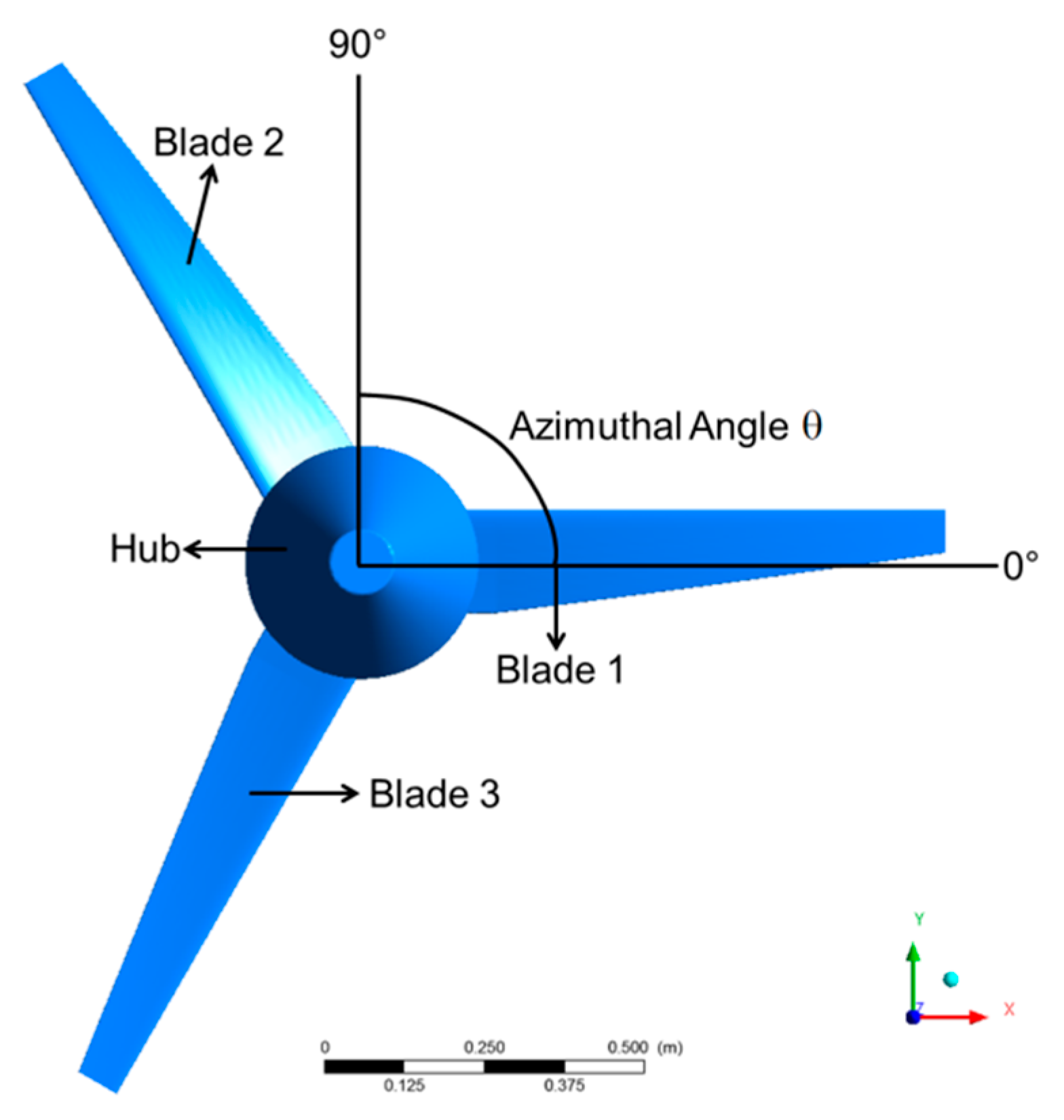
Figure 4.
The rotor view illustrating the blades’ position and the employed coordinate system. Blades rotate counterclockwise.
Figure 4.
The rotor view illustrating the blades’ position and the employed coordinate system. Blades rotate counterclockwise.

Figure 5.
The power coefficient at λ = 5.7 for the three studied configurations, SP, SI15 (15°) and SI30 (30°) inclined with respect to the flow direction: (a) one blade; (b) complete turbine.
Figure 5.
The power coefficient at λ = 5.7 for the three studied configurations, SP, SI15 (15°) and SI30 (30°) inclined with respect to the flow direction: (a) one blade; (b) complete turbine.

Figure 6.
The thrust coefficient at λ = 5.7 for the three studied configurations, SP, SI15 (15°) and SI30 (30°) inclined with respect to the flow direction: (a) one blade; (b) complete turbine.
Figure 6.
The thrust coefficient at λ = 5.7 for the three studied configurations, SP, SI15 (15°) and SI30 (30°) inclined with respect to the flow direction: (a) one blade; (b) complete turbine.

Figure 7.
The drag coefficient at λ = 5.7 for the three studied configurations, SP, SI15 (15°), and SI30 (30°) inclined with respect to the flow direction: (a) one blade; (b) complete turbine.
Figure 7.
The drag coefficient at λ = 5.7 for the three studied configurations, SP, SI15 (15°), and SI30 (30°) inclined with respect to the flow direction: (a) one blade; (b) complete turbine.

Figure 8.
The lift coefficient at λ = 5.7 for the three studied configurations, SP, SI15 (15°) and SI30 (30°) inclined with respect to the flow direction: (a) one blade; (b) complete turbine.
Figure 8.
The lift coefficient at λ = 5.7 for the three studied configurations, SP, SI15 (15°) and SI30 (30°) inclined with respect to the flow direction: (a) one blade; (b) complete turbine.

Figure 9.
The pressure coefficient (a–c) and skin friction coefficient (d–f) at the blade’s pressure side in the three considered inclinations.
Figure 9.
The pressure coefficient (a–c) and skin friction coefficient (d–f) at the blade’s pressure side in the three considered inclinations.


Figure 10.
The vorticity isosurface of 1.5 Hz showing the detached boundary layer for the SP (a), SI15 (b), and SI30 (c) configurations from the turbine axis and the blades. The blade tip vortices are clearly visible.
Figure 10.
The vorticity isosurface of 1.5 Hz showing the detached boundary layer for the SP (a), SI15 (b), and SI30 (c) configurations from the turbine axis and the blades. The blade tip vortices are clearly visible.

Figure 11.
The power coefficient versus tip speed ratio for the different configurations.

Figure 12.
The force coefficient versus tip speed ratio for the different configurations: (a) thrust coefficient; (b) drag coefficient; (c) lift coefficient.
Figure 12.
The force coefficient versus tip speed ratio for the different configurations: (a) thrust coefficient; (b) drag coefficient; (c) lift coefficient.

Figure 13.
The evaluation of the correlation , Equation (8), for the inclined turbine configurations. Lines indicate the correlation: 15° inclination: solid line; 30° inclination: dashed line.
Figure 13.
The evaluation of the correlation , Equation (8), for the inclined turbine configurations. Lines indicate the correlation: 15° inclination: solid line; 30° inclination: dashed line.

Figure 14.
The power coefficient versus tip speed ratio for the two evaluated turbulence models. SP and SI30 configurations.
Figure 14.
The power coefficient versus tip speed ratio for the two evaluated turbulence models. SP and SI30 configurations.

Figure 15.
The intermittency contours around the first blade at the mid-span plane: SP (a), SI15 (b), and SI30 (c) configurations. The black color indicates the laminar flow. Flow progresses from bottom to top.
Figure 15.
The intermittency contours around the first blade at the mid-span plane: SP (a), SI15 (b), and SI30 (c) configurations. The black color indicates the laminar flow. Flow progresses from bottom to top.

Figure 16.
The comparison of the experimental measurements and CFD computations performed in this work on the turbine of Bahaj et al. (2007) [34].
Figure 16.
The comparison of the experimental measurements and CFD computations performed in this work on the turbine of Bahaj et al. (2007) [34].
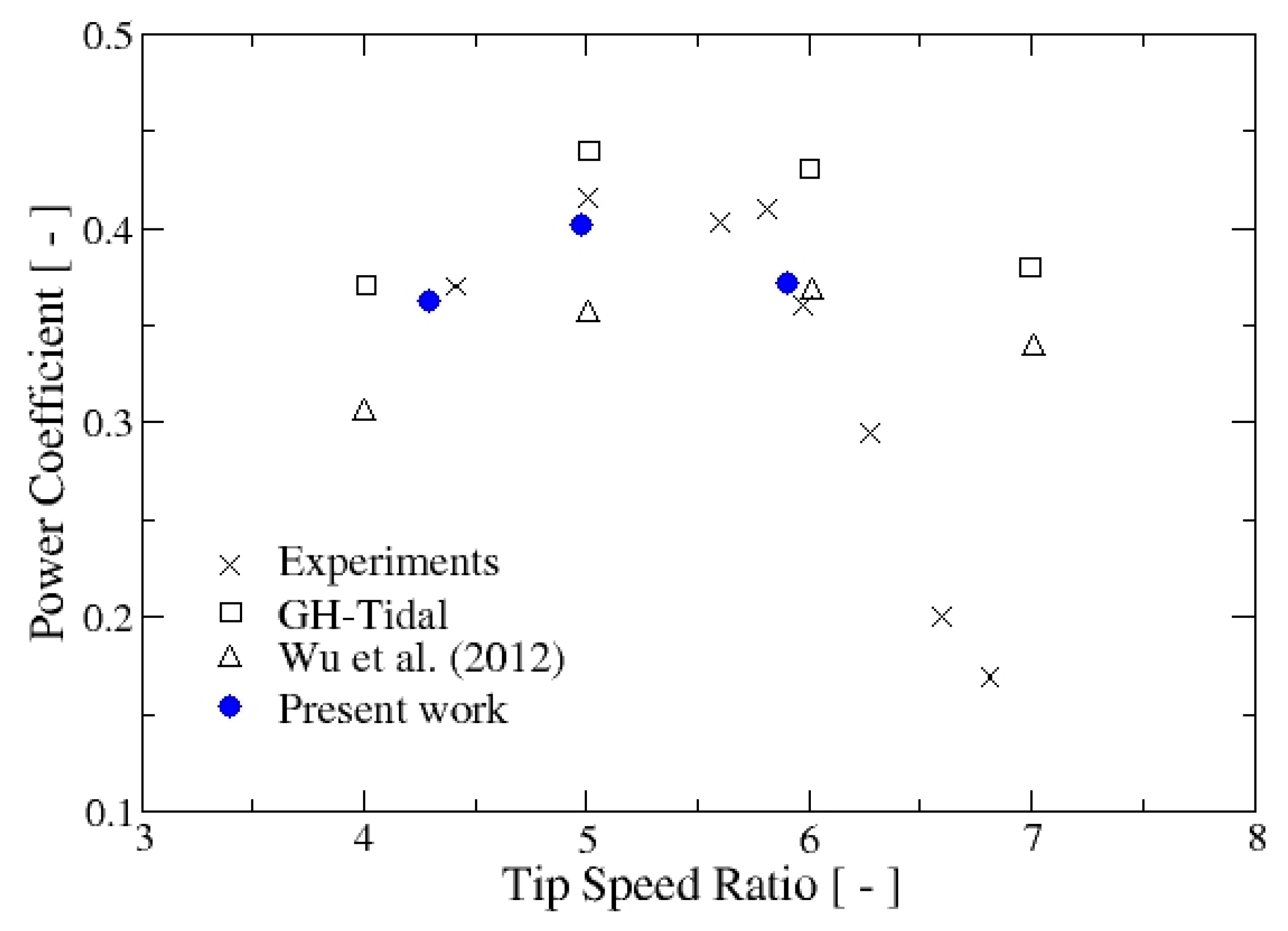
Figure 17.
The comparison of the CFD results obtained in the present study versus the efficiency curve of the IT-PE-100 wind turbine.
Figure 17.
The comparison of the CFD results obtained in the present study versus the efficiency curve of the IT-PE-100 wind turbine.

Figure 18.
The comparison of the CFD results obtained in the present work versus those provided by BEM and LLFVM implemented in the Qblade software. The results computed by the SST Transition turbulence model are also included for reference.
Figure 18.
The comparison of the CFD results obtained in the present work versus those provided by BEM and LLFVM implemented in the Qblade software. The results computed by the SST Transition turbulence model are also included for reference.

Figure 19.
The comparison of the CFD computation of the present study versus the experimental measurements of Reference [19] in a 45° inclined rotor with the incident flow velocity of 0.65 m/s.
Figure 19.
The comparison of the CFD computation of the present study versus the experimental measurements of Reference [19] in a 45° inclined rotor with the incident flow velocity of 0.65 m/s.


Table 1.
The parameters describing the quality of the mesh for the different turbine configurations.
Table 1.
The parameters describing the quality of the mesh for the different turbine configurations.
| Parameter | SP Configuration | SI15 Configuration | SI30 Configuration |
|---|---|---|---|
| Aspect ratio (average) | 0.95 | 0.96 | 0.95 |
| Equiangle skewness (average) | 0.52 | 0.46 | 0.45 |
| Determinant (average) | 0.93 | 0.91 | 0.91 |
| Expansion factor | 1.20 | 1.20 | 1.20 |
© 2018 by the authors. Licensee MDPI, Basel, Switzerland. This article is an open access article distributed under the terms and conditions of the Creative Commons Attribution (CC BY) license (http://creativecommons.org/licenses/by/4.0/).
Share and Cite
MDPI and ACS Style
Contreras, L.T.; Lopez, O.D.; Lain, S. Computational Fluid Dynamics Modelling and Simulation of an Inclined Horizontal Axis Hydrokinetic Turbine. Energies 2018, 11, 3151. https://doi.org/10.3390/en11113151
AMA Style
Contreras LT, Lopez OD, Lain S. Computational Fluid Dynamics Modelling and Simulation of an Inclined Horizontal Axis Hydrokinetic Turbine. Energies. 2018; 11(11):3151. https://doi.org/10.3390/en11113151
Chicago/Turabian StyleContreras, Leidy Tatiana, Omar Dario Lopez, and Santiago Lain. 2018. "Computational Fluid Dynamics Modelling and Simulation of an Inclined Horizontal Axis Hydrokinetic Turbine" Energies 11, no. 11: 3151. https://doi.org/10.3390/en11113151
Note that from the first issue of 2016, this journal uses article numbers instead of page numbers. See further details here.