Total Suspended Particle Emissions Modelling in an Industrial Boiler

Abstract

Particulate matter emission into the atmosphere is a massive-scale problem. Fossil fuel combustion is an important source of this kind of pollution. The knowledge of total suspended particle (TSP) emissions is the first step for TSP control. The formation of TSP emissions is poorly understood; therefore new approaches for TSP emissions source modelling are required. TSP modelling is a multi-variable non-linear problem that would only require basic information on boiler operation. This work reports the development of a non-linear model for TSP emissions estimation from an industrial boiler based on a one-layer neural network. Expansion polynomial basic functions combined with an orthogonal least-square and model structure selection approach were used for modelling. The model required five independent boiler variables for TSP emissions estimation. Data from the data acquisition system of a 350 MW industrial boiler were used for model development and validation. The results show that polynomial expansion basic functions are an excellent approach to solve modelling problems related to complex non-linear systems in the industry.

1. Introduction

Fossil fuels burning in boilers results in the release of combustion gases into the atmosphere containing a gaseous phase and suspended solids or liquid particles pollutants. Environmental regulations have been defined to limit ambient pollutions that can be emitted into the environment around the world.

In order to control pollution in industrial boilers, the first step is to employ an adequate measurement system. A typical system for polluting emissions measurements in industrial boilers consists of Continuous Emissions Monitoring Systems (CEMS). CEMS are nevertheless operationally expensive, and their readings reliability is sensitive to environmental conditions, with difficulties related to their installation and maintenance. Predictive Emissions Monitoring Systems (PEMS) are a recent approach solution planned to replace online analyzers like CEMS by estimating emissions concentrations from process data. PEMS provide a relationship between the process and the emissions through nonlinear modelling data.

Methods based on the use of measurements data from a process have been used for process modelling. Modelling based on linear systems are popular for their simplicity; however, in complex problems with strong non-linearity, the results are limited. It is necessary, then, to develop methodologies that allow non-linear modeling, seeking to preserve the advantages of linear models.

There are different tools to solve the modelling identification problem, depending on the system complexity and knowledge. If the identification is based only on input and output measured data, considering there is no knowledge about the system physics, the identification process is classically called black box modelling. When detail system physics is known, purely mathematical models can be calculated, and the identification process is called white box modelling.

In the process of modelling pollutant emissions in the combustion process, it is practically impossible to have the knowledge of all the thermal, physical, and chemical processes that could exist, and, although this knowledge is available, it is always dispersed. This complicates the development of a complete description of the system in terms of a continuous-time mathematical model. Transferring the knowledge required for a description in discrete time is often difficult, since it is often lost in the process of discretization. Getting a black box model in complex systems is not easy to achieve, even if one has experience and knowledge of the system. Although the basic understanding of the system dynamics sometimes is not available, it is always useful and helps to establish the model structure.

Air quality is a widespread concern, which is generated mainly by population centralization in large cities, which increases traffic, industrialization, and the indiscriminate use of conventional energy [1,2]. Technological advances and the development of clean energy are outweighed by the indiscriminate use of fossil fuels. As a result, the emission of dangerous particles into the atmosphere is increasing [3], having catastrophic effects on all scales and bringing unimaginable damage to public health [4]. Environmental pollution is regulated by global organizations, but most countries do not satisfy the requirements [1,5], and, in addition, in some cases there are records of measurements that widely exceed the limits, thereby causing millions of deaths [4,6,7]. One of the most dangerous environmental pollutants with indiscriminate emissions is particulate matter (PM), which includes large particles (PM₁₀), small particles (PM_2.5), and fine particles (<100 nm) that are not regulated [8], which makes the problem larger [9]. A World Health Organization report on environmental atmosphere contamination stated that the average density of PM₁₀ was augmented about 5% between 2008 and 2013 in 720 cities around the world [10]. It has been reported that a diminution in the content of PM₁₀ by 5 μg per cubic meter in Europe would avoid between 3000 and 8000 annual premature deaths [11]. Alike estimates for PM_2.5 advise a decrease of 7 to 8 months in the life likelihood [12]. In equivalent studies of fine particulate matter, it is estimated that they also increase the damage to health together with large particles, whose health effect is known, and, in consequence, are expected to increase the costs to maintain public health and avoid premature deaths [6].

Total suspended particles (TSP) emissions formation is widely reported but poorly understood. In order to reduce TSP emissions, theoretical TSP generation models have been studied [13] and mainly discuss theories for linking discrete to continuum modelling but do not propose a general theory at the micro- and macroscale levels. Regression modelling of the spatial particulate matter has been developed [14] for modelling the concentrations of suspended particles in the time and space domains in specific localities with a high population concentration. The studies on modelling TSP emissions generally focus on analyzing the effects of suspended particles on the population health [15,16,17,18,19,20]. Modelling of TSP emission sources has been studied [21], conducting research on source apportionment of ambient particulate matter in Europe using receptor models such as principal component analysis, enrichment factors, classical factor analysis, and positive matrix factorization, [22] and building and applying a numerical air quality model that relies on scientific first principles to predict the concentration particles. A study [23] reported a computer-controlled ambient-simulation method to determine the source characteristic profiles of emissions from an oil-fired boiler through isokinetic withdrawal.

In relation to non-linear modelling, artificial neural networks (ANN) are widely applied in engineering processes, in particular for TSP modelling, and neural networks with retro-propagation, such as multi-layer perceptron (MLP), are the most used. However, there is a great diversity of types of neural networks for non-linear modelling based on data. For instance, Ye [24] presented Bayesian–Gaussian neural networks (BGNN), a new methodology for the application of neural networks improved in training time, minimum location, and auto-tuning for online applications. A redefinition of the BGNN algorithm was presented by Liu [25] using genetic algorithms (GA) for the offline adjustment of the threshold matrix and a sliding data window for online applications suitable for non-linear systems that change over time, a feature that makes this algorithm very attractive for online dynamic systems modelling.

The radial basic function (RBF) network offers an alternative in signal processing applications using two-layer neural networks. Common learning algorithms for the RBF network are based on the selection of random functions centers, which has some drawbacks. Reference [26] presents a method using orthogonal least squares, selecting the basic functions centers radially one by one, until an adequate network is built. Kassam [27] presents a training algorithm for the RBF network based on the stochastic gradient (SG) error and shows its versatility in non-linear signal processing applications. Because of its numerical features, the stochastic gradient algorithm is a training algorithm widely used in networks with adaptive radial basis functions, but it presents a compromise between convergence speed and precision due to fixed values in the steps size. Zeng [28] solved this problem by presenting the convex combination of multiple RBF (MCRBF) network algorithm, applying the SG learning algorithm and varying the configuration parameters.

The Volterra polynomials have also been used for system identification [29]. Here, the orthogonal least-squares method is used for offline model framework determination.

Considering that the combustion process is complex, multivariable, and non-linear, which hinders the application of white-box modelling techniques, fitting models for PEMS development is a challenge. The goal of this work was to develop a nonlinear model for TSP emissions in a 350 MW conventional boiler that burns heavy fuel oil in order to provide a good TSP prediction that can be used in PEMS applications using operational boiler data. The non-linear model proposed is based on the polynomial expansion of a multiple-variable function in the neural network framework, considering that there is a finite number of basic functions for an ANN to estimate a non-linear function. The orthogonal least-squares algorithm was used as a parameter estimator because it allows to easily determine a reduced subset of basic functions that best represent the TSP emission dynamics. A classical MLP three-layer ANN was implemented and compared with the polynomial expansion network proposed.

2. Methodology

Regardless of the fact that all systems are non-linear, most of the literature on systems identification refers to the identification of linear systems. The main reason for this is that the assumptions may become very restrictive because of the process complexity, which forces the designer to use strong simplifications or fix the model components. Also, process innovation for improvement together with diverse local environments often results in significant differences between two apparently similar plants.

Power plant equipment and installation are usually fitted to suit the local conditions of a specific place. The construction depends on factors such as fuel availability, innovations and local ambient conditions towards better thermal efficiency and emission control, etc. To make the existing models adequate for different constructions, redesigning and tuning are required. Model equations solving might also add problems to highly detailed first-principle models. Mathematical knowledge is required to develop the model, and time-consuming interactive computations need to be performed.

Identification is the experimental approach to process modelling [30,31]; this approach includes the following steps:

• Experimentation
• Structure model selection
• Parameter estimation
• Model validation

An experimental design must be carried out in order to obtain data that represent the behavior of the process in the whole operating field of the dynamic system. In other words, it is necessary to establish physically support values throughout the input range and measure the effect on the output. The corresponding input and output data sets are finally used to infer a system model. Some parameters to be defined in the experimental phase are: tests preparation, sampling time choice, suitable experiments design, and data pre-processing. Pre-processing data includes, for example, testing the response time, removal of irregularities, control of noise and another unexpected behaviors of the data.

Defining the model framework is called structure model selection. That is a framework that must be explored to get a good model where the model input–output signals and the internal interaction of the model are determined. The model structure is derived using prior knowledge. In general, structure model selection implies the selection of the model approach (multilayer perceptron networks, radial basis function, etc.) considered appropriate to describe the system, and the selection of a subset of this structure model defining the appropriate number of parameters for a specific problem.

The values of the unknown parameters of a parametrized model structure are estimated. Normally, the model that best performs according to the design specifications is chosen. The design specifications can be expressed in many different forms; preferably, they should be formulated with the final model application in mind. In general, the model is selected on the basis of the best possible model predictions following some criterion of error magnitude measurement between the observed output and the model estimation. The method for calculating the model parameters of the selected structure is developed according to the statistical theory and is called estimation. The equivalent process in the ANN theory is often denominated training or learning.

Once the model has been determined, it must be tested to verify whether it meets the design specifications, by evaluating precision, robustness, convergence, and good generalization abilities (interpolation). Validation is closely related to the final model application. The validation criteria of the tracking error compensation algorithm will be defined on the basis of the characteristics of the current compensation algorithms of relevance.

2.1. Polynomial Basic Functions

The model structure is a candidate model set, i.e., a set within which a model must be sought. In general, the problem with the model selection implies a model family selection. For TSP modelling, a polynomial expansions network was used as a model family because of its ability to model non-linear dynamics.

Consider a non-linear dynamic multiple-inputs–simple-output (MISO) system, which is represented by

$${\mathrm{y}}_{\mathrm{t}}=\mathrm{f}\left({\mathrm{u}}_1\left(1\right),{\mathrm{u}}_1\left(2\right),\dots ..,{\mathrm{u}}_1\left(\mathrm{t}-{\mathrm{n}}_1\right),\cdots ,{\mathrm{u}}_{\mathrm{m}}\left(1\right),{\mathrm{u}}_{\mathrm{m}}\left(2\right),\dots ..,{\mathrm{u}}_{\mathrm{m}}\left(\mathrm{t}-{\mathrm{n}}_{\mathrm{m}}\right)\right),$$

(1)

where $\mathrm{f}(·)$ is a non-linear function, $\mathrm{u}$ is the input vector, ${\mathrm{n}}_{\mathrm{p}}$ is the delay samples number in the p-th input, and $\mathrm{m}$ is the input variable number.

Define ${\mathrm{u}}_{\mathrm{t}}$ as

$${\mathrm{u}}_{\mathrm{t}}=\left[{\mathrm{u}}_1\left(1\right),{\mathrm{u}}_1\left(2\right),\dots ..,{\mathrm{u}}_1\left(\mathrm{t}-{\mathrm{n}}_1\right),\cdots ,{\mathrm{u}}_{\mathrm{m}}\left(1\right),{\mathrm{u}}_{\mathrm{m}}\left(2\right),\dots ..,{\mathrm{u}}_{\mathrm{m}}\left(\mathrm{t}-{\mathrm{n}}_{\mathrm{m}}\right)\right],$$

(2)

re-index ${\mathrm{u}}_{\mathrm{t}}$ as

$${\mathrm{u}}_{\mathrm{t}}=\left[{\mathrm{u}}_1,{\mathrm{u}}_2,\cdots ,{\mathrm{u}}_{\mathrm{n}}\right],$$

(3)

where $\mathrm{n}={\mathrm{n}}_1+{\mathrm{n}}_2+\cdots +{\mathrm{n}}_{\mathrm{m}}$, and the Equation (1) is

$${\mathrm{y}}_{\mathrm{t}}=\mathrm{f}\left({\mathrm{u}}_{\mathrm{t}}\right).$$

(4)

Polynomial multivariable expansions have been suggested as candidate base functions [32,33] and they are usually applied in function structure, mainly in one-input variable functions [34]. Recently, the polynomial basis function (PBF), in the multivariable functions context, has been launched within the neural network model structure. Its functional representation is described by

$$\mathrm{f}\left({\mathrm{u}}_{\mathrm{t}}\right)=\hat{\mathrm{f}}\left({\mathrm{u}}_{\mathrm{t}},\mathsf{\Theta }\right)+\mathrm{e}\left({\mathrm{u}}_{\mathrm{t}}^{\mathrm{k}}\right),$$

(5)

$$\begin{gathered} \hat{\mathrm{f}}\left({\mathrm{u}}_{\mathrm{t}},\mathsf{\Theta }\right)={\mathsf{\theta }}_0+{{\displaystyle \sum }}_{\mathrm{i}=1}^{\mathrm{n}}{\mathsf{\theta }}_{\mathrm{i}}{\mathrm{u}}_{\mathrm{i}}+{{\displaystyle \sum }}_{{\mathrm{i}}_1=1}^{\mathrm{n}}{{\displaystyle \sum }}_{{\mathrm{i}}_2={\mathrm{i}}_1}^{\mathrm{n}}{\mathsf{\theta }}_{{\mathrm{i}}_1{\mathrm{i}}_2}{\mathrm{u}}_{{\mathrm{i}}_1}{\mathrm{u}}_{{\mathrm{i}}_2}+ \\ \cdots +{{\displaystyle \sum }}_{{\mathrm{i}}_1=1}^{\mathrm{n}}{{\displaystyle \sum }}_{{\mathrm{i}}_2={\mathrm{i}}_1}^{\mathrm{n}}\cdots {{\displaystyle \sum }}_{{\mathrm{i}}_{\mathrm{k}}={\mathrm{i}}_{\mathrm{k}-1}}^{\mathrm{n}}{\mathsf{\theta }}_{{\mathrm{i}}_1{\mathrm{i}}_2\cdots {\mathrm{i}}_{\mathrm{k}}}{\mathrm{u}}_{{\mathrm{i}}_1}{\mathrm{u}}_{{\mathrm{i}}_2}\cdots {\mathrm{u}}_{{\mathrm{i}}_{\mathrm{k}}}={{\displaystyle \sum }}_{\mathrm{j}=1}^{\mathrm{N}}{\mathsf{\theta }}_{\mathrm{j}}{\mathsf{\phi }}_{\mathrm{j}}\left({\mathrm{u}}_{\mathrm{t}}\right), \end{gathered}$$

(6)

where $\mathsf{\Theta }=\left\{{\mathsf{\theta }}_{\mathrm{j}}\right\}$ is the concatenated parameters, $\left\{{\mathsf{\phi }}_{\mathrm{j}}\right\}$ is the set of basic functions formed from the polynomial input terms, $\mathrm{N}=\frac{\left(\mathrm{n}+\mathrm{k}\right)!}{\mathrm{n}!\mathrm{k}!}$ is the polynomial basic functions number, $\mathrm{k}$ is the polynomial expansion order, and $\mathrm{e}\left({\mathrm{u}}_{\mathrm{t}}^{\mathrm{k}}\right)$ indicates the approximation error generated by the order $\mathrm{k}$ from the input vector. The basic functions are polynomials of some specific order of the input vector ${\mathrm{u}}_{\mathrm{t}}\in {ℛ}^{\mathrm{n}}$. This process can be viewed as the transformation of the multivariable input vector to a space of higher dimensions.

There are a certain number of basic functions to approximate a non-linear function with accuracy [35]. However, a practical method is necessary to determine these basic functions. The necessary approximation precision can be achieved by an acceptable number of linearly independent non-linear basic functions.

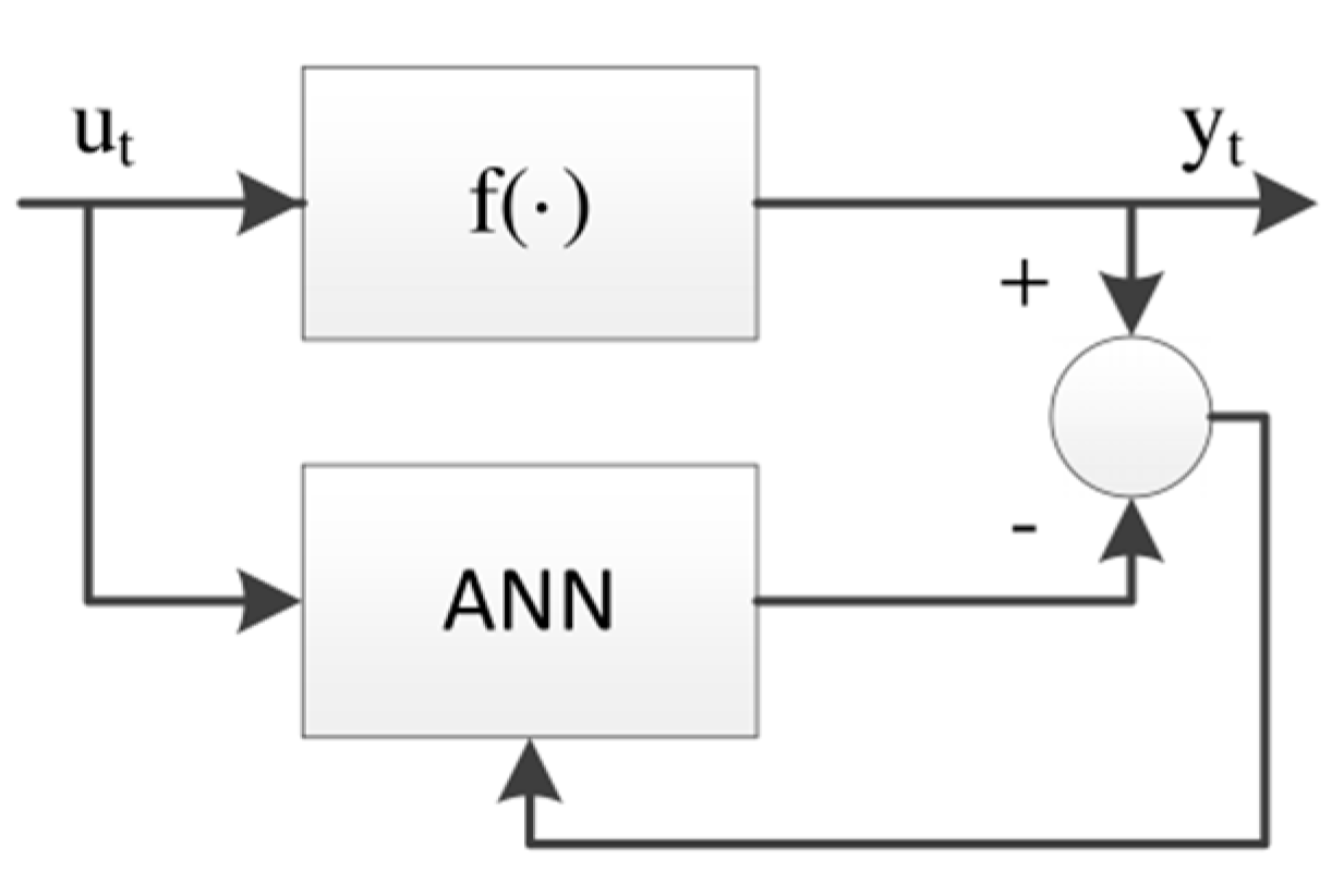
Polynomial expansion base functions offer a good approximation of non-linear functions. The structure of non-linear identification is shown in Figure 1. It is assumed that the non-linear function $\hat{\mathrm{f}}(·)$ in the polynomial expansion basic functions is estimated by a single-layer ANN, which is a linear combination of non-linear polynomials.

With the increase in order $\mathrm{k}$, the basic functions number $\mathrm{N}$ gets bigger and bigger. So, the problem is function $\hat{\mathrm{f}}\left({\mathrm{u}}_{\mathrm{t}}\right)$ estimation using a suitable ANN, dimensioned such that the estimate precision is according to the specified requirements. The framework model selection and parameters estimation of one-layer ANN are detailed here.

2.2. Model Structure Selection and Parameter Estimation

Obtaining the model that represents the TSP emissions dynamic of a boiler with good precision is a problem that requires looking for the best model structure, which means defining the number of parameters (basic functions) appropriate for the model and estimating the parameters to obtain exact values for the model.

There are many ways to the selection of basic functions. In this case, the structure selection was executed offline using the orthogonal least-squares algorithm [36] to determine the more meaningful basic functions number for TSP modelling.

This assumes that the data $\left({\mathrm{y}}_{\mathrm{t}},{\mathrm{u}}_{\mathrm{t}},\mathrm{t}=1,2,\cdots ,\mathrm{M}\right)$ from the input and output systems are known. On the basis of Equation (6), the estimation function can be formulated in vector form through:

$$\mathrm{Y}=\mathsf{\Phi }\left(\mathrm{u}\right)\mathsf{\Theta }+\mathrm{E}\left({\mathrm{u}}^{\mathrm{k}}\right),$$

(7)

where the input vector $\mathrm{Y}∊{ℛ}^{\mathrm{M}\times 1}$, the parameter vector $\mathsf{\Theta }∊{ℛ}^{\mathrm{N}\times 1}$, the error vector $\mathrm{E}\left({\mathrm{u}}^{\mathrm{k}}\right)∊{ℛ}^{\mathrm{M}\times 1}$, and the basic functions matrix $\mathsf{\Phi }∊{ℛ}^{\mathrm{M}\times \mathrm{N}}$ are

$$\mathrm{Y}={\left[{\mathrm{y}}_1{\mathrm{y}}_2\cdots {\mathrm{y}}_{\mathrm{M}}\right]}^{\mathrm{T}},$$

(8)

$$\mathsf{\Theta }={\left[{\mathsf{\theta }}_1{\mathsf{\theta }}_2\cdots {\mathsf{\theta }}_{\mathrm{N}}\right]}^{\mathrm{T}},$$

(9)

$$\mathrm{E}\left({\mathrm{u}}^{\mathrm{k}}\right)={\left[\mathrm{e}\left({\mathrm{u}}_1^{\mathrm{k}}\right)\mathrm{e}\left({\mathrm{u}}_2^{\mathrm{k}}\right)\cdots \mathrm{e}\left({\mathrm{u}}_{\mathrm{M}}^{\mathrm{k}}\right)\right]}^{\mathrm{T}},$$

(10)

$$\mathsf{\Phi }\left(\mathrm{x}\right)=\left[\begin{array}{ccc}\begin{array}{c}{\mathsf{\phi }}_1\left({\mathrm{u}}_1\right)\\ {\mathsf{\phi }}_1\left({\mathrm{u}}_2\right)\\ \begin{array}{c}⋮\\ {\mathsf{\phi }}_1\left({\mathrm{u}}_{\mathrm{M}}\right)\end{array}\end{array}& \begin{array}{c}{\mathsf{\phi }}_2\left({\mathrm{u}}_1\right)\\ {\mathsf{\phi }}_2\left({\mathrm{u}}_2\right)\\ \begin{array}{c}⋮\\ {\mathsf{\phi }}_2\left({\mathrm{u}}_{\mathrm{M}}\right)\end{array}\end{array}& \begin{array}{cc}\begin{array}{c}\cdots \\ \cdots \\ \begin{array}{c}\ddots \\ \cdots \end{array}\end{array}& \begin{array}{c}{\mathsf{\phi }}_{\mathrm{N}}\left({\mathrm{u}}_1\right)\\ {\mathsf{\phi }}_{\mathrm{N}}\left({\mathrm{u}}_2\right)\\ \begin{array}{c}⋮\\ {\mathsf{\phi }}_{\mathrm{N}}\left({\mathrm{u}}_{\mathrm{M}}\right)\end{array}\end{array}\end{array}\end{array}\right].$$

(11)

The parameter vector $\mathsf{\Theta }$ is generally found by optimizing the error vector norm, that is,

$$\hat{\mathsf{\Theta }}={\mathrm{argmin}}_{\mathrm{W}}||\mathrm{Y}-\mathsf{\Phi }\left(\mathrm{u}\right)\mathrm{W}||{}_2,$$

(12)

obtaining the least-squares solution.

The vector of ${\mathsf{\Phi }}_{\mathrm{i}}={\left[{\mathsf{\phi }}_{\mathrm{i}}\left({\mathrm{u}}_1\right),{\mathsf{\phi }}_{\mathrm{i}}\left({\mathrm{u}}_2\right),\cdots ,{\mathsf{\phi }}_{\mathrm{i}}\left({\mathrm{u}}_{\mathrm{M}}\right)\right]}^{\mathrm{T}}$, for $\mathrm{i}=1,2,\cdots ,\mathrm{N}$, forms a basic vector set, and the orthogonal least-squares solution $\hat{\mathsf{\Theta }}$ satisfies the condition that $\mathsf{\Phi }\left(\mathrm{u}\right)\hat{\mathsf{\Theta }}$ will be the projection of $\mathrm{Y}$ on the space generated by the basic function vectors $\left\{{\mathsf{\Phi }}_{\mathrm{i}}\right\}$. The orthogonal least-squares method implies the basic vector set transformation $\left\{{\mathsf{\Phi }}_{\mathrm{i}}\right\}$ into an orthogonal basic vector set, and, therefore, makes it possible to compute the individual impact on the output, for all base vectors. An orthogonal factorization of $\mathsf{\Phi }\left(\mathrm{u}\right)$ can be obtained by means of a construction known as Gram–Schmidt orthogonalization process.

First, set ${\mathrm{P}}_1={\mathsf{\Phi }}_1$. The following vectors are then given inductively in the following way: suppose that ${\mathrm{P}}_1,\cdots ,{\mathrm{P}}_{\mathrm{m}}\left(1\le \mathrm{m}\le \mathrm{n}\right)$ have been chosen, so that for each $\mathrm{k}$ $\left\{{\mathrm{P}}_1,\cdots ,{\mathrm{P}}_{\mathrm{m}}\right\},\left(1\le \mathrm{k}\le \mathrm{m}\right)$ is an orthogonal base for the vector subspace that is generated by that ${\mathsf{\Phi }}_1,\cdots ,{\mathsf{\Phi }}_{\mathrm{k}}$. For building the next vector ${\mathrm{P}}_{\mathrm{m}+1}$, set

$${\mathrm{P}}_{\mathrm{m}+1}={\mathsf{\Phi }}_{\mathrm{m}+1}-{{\displaystyle \sum }}_{\mathrm{k}=1}^{\mathrm{m}}\frac{{\mathsf{\Phi }}_{\mathrm{m}+1},{\mathrm{P}}_{\mathrm{k}}}{||{\mathrm{P}}_{\mathrm{k}}||{}^2}{\mathrm{P}}_{\mathrm{k}},$$

(13)

So ${\mathrm{P}}_{\mathrm{m}+1}\ne 0$, since, otherwise, ${\mathrm{P}}_{\mathrm{m}+1}$ is a linear combination of ${\mathrm{P}}_1,\cdots ,{\mathrm{P}}_{\mathrm{m}}$.

Furthermore, if $1\le \mathrm{j}\le \mathrm{m}$, then

$$\langle {\mathrm{P}}_{\mathrm{m}+1},{\mathrm{P}}_{\mathrm{j}}\rangle =\langle {\mathsf{\Phi }}_{\mathrm{m}+1},{\mathrm{P}}_{\mathrm{j}}\rangle -{{\displaystyle \sum }}_{\mathrm{k}=1}^{\mathrm{m}}\frac{\langle {\mathsf{\Phi }}_{\mathrm{m}+1},{\mathrm{P}}_{\mathrm{k}}\rangle }{||{\mathrm{P}}_{\mathrm{k}}||{}^2}\langle {\mathrm{P}}_{\mathrm{k}},{\mathrm{P}}_{\mathrm{j}}\rangle =\langle {\mathsf{\Phi }}_{\mathrm{m}-1},{\mathrm{P}}_{\mathrm{j}}\rangle -\langle {\mathsf{\Phi }}_{\mathrm{m}-1},{\mathrm{P}}_{\mathrm{j}}\rangle =0.$$

(14)

Therefore, $\left\{{\mathrm{P}}_1,\cdots ,{\mathrm{P}}_{\mathrm{m}+1}\right\}$ is an orthogonal set consisting of $\mathrm{m}+1$ nonzero vectors in the subspace generated by ${\mathsf{\Phi }}_1,\cdots ,{\mathsf{\Phi }}_{\mathrm{m}+1}$. Because orthogonal nonzero vectors are linearly independent, this is a base for this subspace. So, the vectors ${\mathrm{P}}_1,\cdots ,{\mathrm{P}}_{\mathrm{n}}$ can be constructed one after the other according to the Equation (14). In general, we have, for $\mathrm{n}$ = N:

$${\mathrm{P}}_1={\mathsf{\Phi }}_1,$$

(15)

$${\mathrm{P}}_2={\mathsf{\Phi }}_2-\frac{\langle {\mathsf{\Phi }}_2,{\mathrm{P}}_1\rangle }{||{\mathrm{P}}_1||{}^2}{\mathrm{P}}_1,$$

(16)

$${\mathrm{P}}_3={\mathsf{\Phi }}_3-\frac{\langle {\mathsf{\Phi }}_3,{\mathrm{P}}_1\rangle }{||{\mathrm{P}}_1||{}^2}{\mathrm{P}}_1-\frac{\langle {\mathsf{\Phi }}_3,{\mathrm{P}}_2\rangle }{||{\mathrm{P}}_2||{}^2}{\mathrm{P}}_2,$$

(17)

$${\mathrm{P}}_{\mathrm{N}}={\mathsf{\Phi }}_{\mathrm{N}}-{{\displaystyle \sum }}_{\mathrm{k}=1}^{\mathrm{N}-1}\frac{\langle {\mathsf{\Phi }}_{\mathrm{N}},{\mathrm{P}}_{\mathrm{k}}\rangle }{||{\mathrm{P}}_{\mathrm{k}}||{}^2}{\mathrm{P}}_{\mathrm{k}}.$$

(18)

The matrix $\mathsf{\Phi }\left(\mathrm{u}\right)$ can be written as

$$\mathsf{\Phi }\left(\mathrm{u}\right)=\mathrm{PQ},$$

(19)

where the matrix $\mathrm{P}=\left[{\mathrm{P}}_1,{\mathrm{P}}_2,\cdots ,{\mathrm{P}}_{\mathrm{N}}\right]$ has the size $\mathrm{M}\times \mathrm{N}$ with orthogonal columns, and $\mathrm{Q}$ is a unitary $\mathrm{N}\times \mathrm{N}$ upper triangular matrix with 1 on the main diagonal and 0 below the main diagonal.

$$\mathrm{Q}=\left[\begin{array}{ccc}\begin{array}{ccc}1& \frac{\langle {\mathsf{\Phi }}_2,{\mathrm{P}}_1\rangle }{||{\mathrm{P}}_1||{}^2}{\mathrm{P}}_1& \frac{\langle {\mathsf{\Phi }}_3,{\mathrm{P}}_1\rangle }{||{\mathrm{P}}_1||{}^2}{\mathrm{P}}_1\\ 0& 1& \frac{\langle {\mathsf{\Phi }}_3,{\mathrm{P}}_2\rangle }{||{\mathrm{P}}_2||{}^2}{\mathrm{P}}_1\\ 0& 0& 1\end{array}& \cdots & \begin{array}{c}\frac{\langle {\mathsf{\Phi }}_{\mathrm{N}},{\mathrm{P}}_1\rangle }{||{\mathrm{P}}_1||{}^2}{\mathrm{P}}_1\\ \frac{\langle {\mathsf{\Phi }}_{\mathrm{N}},{\mathrm{P}}_2\rangle }{||{\mathrm{P}}_2||{}^2}{\mathrm{P}}_2\\ \frac{\langle {\mathsf{\Phi }}_{\mathrm{N}},{\mathrm{P}}_{\mathrm{N}-1}\rangle }{||{\mathrm{P}}_{\mathrm{N}-1}||{}^2}{\mathrm{P}}_{\mathrm{N}-1}\end{array}\\ ⋮& \ddots & ⋮\\ \begin{array}{ccc}0\hspace{1em}\hspace{1em} & 0\hspace{1em}\hspace{1em}\hspace{1em}& 0\hspace{1em}\hspace{1em}\hspace{1em}\end{array}& \cdots & 1\end{array}\right].$$

(20)

The properties of orthogonality of $\mathrm{P}$ are advantageous from the logarithmic point of view, in such a way that Equation (7) can be represented by

$$\mathrm{Y}=\mathrm{PQ}\mathsf{\Theta }+\mathrm{E}\left({\mathrm{u}}^{\mathrm{k}}\right),$$

(21)

and, defining $\mathrm{W}=\mathrm{Q}\mathsf{\Theta },$ the Equation (21) can be represented by

$$\mathrm{Y}=\mathrm{PW}+\mathrm{E}\left({\mathrm{u}}^{\mathrm{k}}\right),$$

(22)

and

$$\mathsf{\Theta }={\mathrm{Q}}^{-1}\mathrm{W},$$

(23)

where $\mathrm{W}={\left[{\mathrm{w}}_1,{\mathrm{w}}_2,\cdots ,{\mathrm{w}}_{\mathrm{N}}\right]}^{\mathrm{T}}∊{\mathrm{R}}^{\mathrm{N}\times 1}.$The vector $\mathrm{W}$ can be deduced as the optimal estimate $\hat{\mathrm{W}}={\left[{\hat{\mathrm{w}}}_1,{\widehat{w}}_2,\cdots ,{\hat{\mathrm{w}}}_{\mathrm{N}}\right]}^{\mathrm{T}}$ as follows:

From Equation (22), $$ can be represented by

$$\hat{\mathrm{Y}}=\mathrm{P}\hat{\mathrm{W}},$$

(24)

pre-multiplying Equation (24) by ${\mathrm{P}}^{\mathrm{T}}$

$${\mathrm{P}}^{\mathrm{T}}\hat{\mathrm{Y}}={\mathrm{P}}^{\mathrm{T}}\mathrm{P}\hat{\mathrm{W}},$$

(25)

in vector form

$$\left[\begin{array}{c}{\mathrm{P}}_1^{\mathrm{T}}\hat{\mathrm{Y}}\\ ⋮\\ {\mathrm{P}}_{\mathrm{N}}^{\mathrm{T}}\hat{\mathrm{Y}}\end{array}\right]=\left[\begin{array}{c}{\mathrm{P}}_1^{\mathrm{T}}{\mathrm{P}}_1{\hat{\mathrm{w}}}_1\\ ⋮\\ {\mathrm{P}}_{\mathrm{N}}^{\mathrm{T}}{\mathrm{P}}_{\mathrm{N}}{\hat{\mathrm{w}}}_{\mathrm{N}}\end{array}\right],$$

(26)

$${\hat{\mathrm{w}}}_{\mathrm{i}}=\frac{{\mathrm{P}}_{\mathrm{i}}^{\mathrm{T}}\mathrm{Y}^}{{\mathrm{P}}_{\mathrm{i}}^{\mathrm{T}}{\mathrm{P}}_{\mathrm{i}}},\mathrm{for}\mathrm{i}=1,2,\cdots ,\mathrm{N}.$$

(27)

So, $||\mathrm{Y}-{\mathrm{P}\hat{\mathrm{W}}||}_2$ is minimal. The equivalent optimal parameters vector is

$$\hat{\mathsf{\Theta }}={\mathrm{Q}}^{-1}\hat{\mathrm{W}}.$$

(28)

The orthogonalization Gram–Schmidt algorithm can be applied to calculate Equation (28), therefore, to solve the least squares algorithm and to estimate $\hat{\mathsf{\Theta }}$ and evaluate the variance for each basic function ${\mathsf{\phi }}_{\mathrm{i}}$.

The variance of the output can be written as

$$\frac{1}{\mathrm{M}}{\mathrm{Y}}^{\mathrm{T}}\mathrm{Y}=\frac{1}{\mathrm{M}}{\displaystyle \sum }_{\mathrm{i}=1}^{\mathrm{N}}{\mathrm{w}}_{\mathrm{i}}^2{\mathrm{P}}_{\mathrm{i}}^{\mathrm{T}}{\mathrm{P}}_{\mathrm{i}}+\frac{1}{\mathrm{M}}{\left(\mathrm{E}\left({\mathrm{u}}^{\mathrm{k}}\right)\right)}^{\mathrm{T}}\mathrm{E}\left({\mathrm{u}}^{\mathrm{k}}\right).$$

(29)

Note that ${\displaystyle \sum }_{\mathrm{i}=1}^{\mathrm{N}}{\mathrm{w}}_{\mathrm{i}}^2{\mathrm{P}}_{\mathrm{i}}^{\mathrm{T}}{\mathrm{P}}_{\mathrm{i}}/\mathrm{M}$ is the part of the variance of the looked-for output which can be represented by the basic functions, and ${\mathrm{E}}^{\mathrm{T}}\mathrm{E}/\mathrm{M}$ is the variance not represented by ${\mathrm{y}}_{\mathrm{t}}$. Thus, ${\mathrm{w}}_{\mathrm{i}}^2{\mathrm{P}}_{\mathrm{i}}^{\mathrm{T}}{\mathrm{P}}_{\mathrm{i}}$ is the increment of the variance of the desired output represented by ${\mathrm{P}}_{\mathrm{i}}$, and the reduction ratio of the error due to ${\mathrm{P}}_{\mathrm{i}}$ can be defined by:

$${\mathrm{r}}_{\mathrm{i}}=\frac{{\hat{\mathrm{w}}}_{\mathrm{i}}^2{\mathrm{P}}_{\mathrm{i}}^{\mathrm{T}}{\mathrm{P}}_{\mathrm{i}}}{{\mathrm{Y}}^{\mathrm{T}}\mathrm{Y}},$$

(30)

This ratio allows a simple and efficient mechanism to search for a significant basic functions subset. The implementation is based on the classical Gram–Schmidt method [36,37], see Appendix A.

PBFs order changing will result in an error reduction ratio change, ${\mathrm{r}}_{\mathrm{i}}$. For PBFs, there are $\mathrm{N}!$ combinations; ${\mathrm{r}}_{\mathrm{i}}^{\left(\mathrm{j}\right)}$ denotes the error reduction ${\mathrm{r}}_{\mathrm{i}}$ corresponding to the j-th PBFs arrangement. The conventional Gram–Schmidt algorithm can be applied to find the actual arrangement of the basic functions ${\mathsf{\phi }}_1\left({\mathrm{u}}_{\mathrm{t}}\right),{\mathsf{\phi }}_2\left({\mathrm{u}}_{\mathrm{t}}\right),\cdots ,{\mathsf{\phi }}_{\mathrm{N}}\left({\mathrm{u}}_{\mathrm{t}}\right)$, which represents the best arrangement, in such a way that

$${{\displaystyle \sum }}_{\mathrm{i}=1}^{\mathrm{k}}{\mathrm{r}}_{\mathrm{i}}\ge {{\displaystyle \sum }}_{\mathrm{i}=1}^{\mathrm{k}}{\mathrm{r}}_{\mathrm{i}}^{\left(\mathrm{j}\right)}\mathrm{for}\mathrm{j}\ne 0,\mathrm{j}=1,2,\cdots \mathrm{N}!,\mathrm{k}=1,2,\cdots ,\mathrm{N}.$$

(31)

So, the priority of the basic functions is determined. Therefore, the best PBFs arrangement is denoted by ${\mathsf{\phi }}_1\left({\mathrm{u}}_{\mathrm{t}}\right),{\mathsf{\phi }}_2\left({\mathrm{u}}_{\mathrm{t}}\right),\cdots ,{\mathsf{\phi }}_{\mathrm{N}}\left({\mathrm{u}}_{\mathrm{t}}\right),$ and the corresponding parameter vector is $\mathsf{\Theta }$.

3. TSP Modelling

3.1. TSP Emission Measurement Instrument

A PM instrument was used to measure TSP emissions from 350 MW Unit. The instrument installed is a Neo Laser Dust Long-Path monitor, based on a diode laser technology. The instrument was installed on the appropriate stack elevation to prevent interference with the probe due to problems of flow turbulences, cyclonic flow, and fluctuating PM stratification, see Figure 2. The measuring principle of this instrument is based on the particles property to absorb and scatter transmitted light. A red laser light is transmitted through the process flue gas, and two separate detectors detect the forward scattered light and direct light transmitted. Both signals are functions of the number of dust particles contained in the flue gas. Because of the low range of concentration levels used in the scattering mode, the PM probe was setup to operate on the direct light signal mode. This mode works for an active range from 0 to 10,000 mg/Nm³. Given the known PM emissions range at Unit, the instrument output current loop (from 4 to 20 mA) was adjusted from 0 to 800 mg/Nm³, to increase sensitivity. The response time of this instrument is 1–2 s. The detection limit is 0.5 mg/Nm³, and the accuracy is ±0.5 mg/Nm³ or ±5 percent of the reading, whichever is higher. The PM Neo instrument consists of a transmitter and a receiver unit. Both the transmitter and the receiver are installed onto stack flanges. The optical path length for this probe can be adjusted from 3 to 6 m. For this particular application, it was setup at 5.5 m. The instrument has also an air purging system, preventing dust from fouling the optical windows and interfering with the measurements.

3.2. Experimental Test

The boiler was an opposed wall-fired 350 MW unit, designed and manufactured by Babcock Hitachi. The unit had a balanced draft furnace. The firing system was composed of 12 conventional oil-fired combustion cells (two burners per cell, six cells per wall), with one common secondary air register per burner pairs. Secondary air was introduced at the adjacent side of the combustion walls; however, the wind box was of a wrap-around design to minimize wind-box air stratification. The boiler was a single reheat unit, with hot reheat steam temperatures of 540 °C. The boiler was equipped with flue gas recirculation (FGR) for steam temperature control, as well with attemperating sprays and sootblowers. There was neither particulate nor SO₂ control on this unit. This unit fired Mexican and imported high-sulfur (~3–4 percent sulfur) heavy fuel oil (Bunker C). For testing, TSP data were acquired over a range that included low, mid, and high TSP concentrations. To have good variability in the data, a range of unit operating conditions were used, including economizer oxygen excess, steam atomization pressure, fuel temperature, etc.; more boiler details can be consulted in reference [38]. Figure 2 shows a simplified boiler scheme including the used instruments.

The excess air could be manipulated within the capabilities of the O₂ trim control. Fuel combustion parameters, such as the fuel temperature and the steam atomization pressure variables, could also be manipulated to the maximum extent allowed by the firing system (physical limitations, design parameters, etc.). The FGR damper and secondary air register biasing could be performed within the available capability of the FGR damper and secondary air register control. Non-controllable variables (unit load, fuel flow, etc.) were monitored in order to characterize the effect on TSP emissions. The minimum and maximum levels were determined so not to break any operational constraints imposed by the boiler’s limits (i.e., minimum wind-box pressure, maximum steam temperatures, maximum furnace exit gas temperature, etc.).

Forty-eight parametric tests were performed at full load with all cells in service. For all runs, the main variables data were collected for at least a 15 min, once the steady-state unit condition was achieved. A combination of data were acquired automatically by the data acquisition system (DAS) and the continuous emissions monitoring (CEM) system, including TSP emissions, Unit load (Load), oxygen excess (O₂), atomization pressure (P_atom), fuel mass flow (Q_f), fuel temperature (T_f). The tests at 100 percent load included combinations of oxygen excess, fuel temperature, and atomization pressure. The series of tests conducted at full load to evaluate the effect of atomization pressure and fuel temperature on boiler emissions and performance was accomplished at different levels of excess O₂, in a range from 0.6 to 1.8 percent. Tests with the FGR registers were performed at full load, only to observe the effect on TSP emissions and Unit performance. In the TSP emissions model, the FGR variable was not included, since, at this load, the flue gas recirculation was not manipulated. The influence of the FGR gate opening and levels of excess O₂ in TSP emissions is shown in Figure 3. The average difference in TSP emissions between the open and closed FGR damper conditions was approximately 40 mg/Nm³, significant enough to consider a modified operation with the OFF/ON damper closed. Obviously, the manipulation of this damper modified other important parameters, such as NOx emissions. TSP emissions increased as the FGR gate opened and the main steam temperature control required a higher steam attemperation flow. On the other hand, a greater impact on TSP emissions was observed as the O₂ excess decreased, with a clearly non-linear behavior. Manipulation of the fuel temperature was accomplished at different levels of excess O₂, in a range from 0.6 to 1.7 percent, while the atomization pressure was kept at 15.1 bar and the OFF/ON FGR discharge damper was shut. The effect of the fuel temperature on TSP resulted in an average reduction of approximately 0.8 mg/Nm³ per °C increase in fuel temperature, or a decrease of approximately 20 mg/Nm³ in TSP for the tested range of fuel temperature from 115 to 142 °C.

A series of tests were conducted at full load to evaluate the effect of atomization pressure and fuel temperature on boiler emissions and performance. The manipulation of the atomization pressure was accomplished at different levels of excess O₂ in a range from 0.6 to 1.8 percent, while the fuel temperature was kept at 130.8 °C and the OFF/ON FGR discharge damper was shut. The results of the atomization pressure tests on TSP are shown in Figure 4. The effect of the steam atomization pressure on TSP was of reducing TSP emissions as much as 15 mg/Nm³ per bar increase in the atomization pressure at the low O₂ levels. The effect of steam atomization on nitrogen oxides (NOx) emissions was less significant than for TSP, representing approximately 1% increase in NOx emissions per bar increase in atomization pressure, independent of the excess O₂ level.

3.3. TSP Emissions Modelling and Validation

From the parametric tests results, the variables that had independent effects on TSP emissions in the combustion process of the unit were: O₂ excess, P_atom, T_f, Load, and Q_f. Considering these variables as input, the proposed PBF–ANN was developed. From Equation (2), $\mathrm{m}=5,{\mathrm{n}}_1={\mathrm{n}}_2={\mathrm{n}}_3={\mathrm{n}}_4={\mathrm{n}}_5=1,\mathrm{n}=5$, and ${\mathrm{u}}_{\mathrm{t}}={\left[{\mathrm{u}}_1,{\mathrm{u}}_2,{\mathrm{u}}_3,{\mathrm{u}}_4,{\mathrm{u}}_5\right]}^{\mathrm{T}}$, where ${\mathrm{u}}_1=\mathrm{Load},{\mathrm{u}}_2={\mathrm{Q}}_{\mathrm{f}},{\mathrm{u}}_3={\mathrm{P}}_{\mathrm{atom}},{\mathrm{u}}_4={\mathrm{T}}_{\mathrm{f}},{\mathrm{u}}_5={\mathrm{O}}_2$. Figure 5 shows an outline of the structure of the ANN for the implementation of the model defined in the Equation (6).

The basic functions number of the polynomial expansion for order $\mathrm{k}=3$ is $\mathrm{N}=\frac{\left(5+3\right)!}{5!3!}=$ 56.

The classical Gram–Schmidt method for Equations (A1)–(A11) was implemented in MatLab^® software in order to get the highest priority basic functions subset and parameter estimation $\mathsf{\Theta }$.

The classical MLP–ANN was implemented with input, hidden, and output layers. The input layer had six neurons (one for each model input variable, O₂ excess, P_atom, T_f, Load, and Q_f). The hidden layer was defined with N neurons, and the output layer was with one neuron; the TSP prediction was defined as ${\widehat{\mathrm{TSP}}}_{\mathrm{t}}$. The input to the output relationship is characterized by ${\widehat{\mathrm{PST}}}_{\mathrm{t}}=\frac{1}{1-{\mathrm{e}}^{-{\mathrm{f}}_{\mathrm{s}}}}$, ${\mathrm{f}}_{\mathrm{s}}={\displaystyle \sum }_{\mathrm{i}=1}^{\mathrm{N}}{\mathrm{s}}_{\mathrm{i}}{\hat{\mathrm{v}}}_{\mathrm{i}}+{\hat{\mathrm{v}}}_{\mathrm{N}+1}$, ${\mathrm{s}}_{\mathrm{i}}=\frac{1}{1-{\mathrm{e}}^{-{\mathrm{r}}_{\mathrm{j}}}}$, ${\mathrm{r}}_{\mathrm{j}}={\displaystyle \sum }_{\mathrm{i}=1}^5{\mathrm{x}}_{\mathrm{i}}{\mathrm{w}}_{\mathrm{ij}}+{\mathrm{w}}_{6,\mathrm{j}}$. Figure 6 shows a graphical representation of the MLP–ANN structure.

The MLP model training process was made with a backpropagation algorithm implemented in MatLab^® software (The MathWorks, Inc., Natick, MA, USA) in order to build the model and to evaluate the best hidden layer neural N value for modelling TSP emissions.

In order to model the validation, the set of parametric tests was divided into two subsets: the first subset for the training model (80% of parametric tests) and the second subset for the validation model (20% of parametric tests).

For evaluating the predictive accuracy between the PBF and the MLP models, two statistical metrics were selected: the root-mean-square error (RMSE) and the correlation coefficients (${\mathrm{R}}^2$). ${\mathrm{R}}^2$ indicates the correlation between observed and predicted data, and RMSE measures error-based model accuracy. ${\mathrm{R}}^2$ = 1 gives the results of the predicted value equal to the measured value.

${\mathrm{R}}^2$ is defined as

$${\mathrm{R}}^2=1-\frac{\sqrt{{{\displaystyle \sum }}_{\mathrm{k}=1}^{\mathrm{M}}{\left({\mathrm{y}}_{\mathrm{k}}-{\hat{\mathrm{y}}}_{\mathrm{k}}\right)}^2}}{\sqrt{{{\displaystyle \sum }}_{\mathrm{k}=1}^{\mathrm{M}}{\left({\mathrm{y}}_{\mathrm{k}}-{\overline{\mathrm{y}}}_{\mathrm{k}}\right)}^2}},$$

(32)

and RMSE is

$$\mathrm{RMSE}=\sqrt{\frac{{{\displaystyle \sum }}_{\mathrm{k}=1}^{\mathrm{M}}{\left({\hat{\mathrm{y}}}_{\mathrm{k}}-{\mathrm{y}}_{\mathrm{k}}\right)}^2}{\mathrm{M}}}$$

(33)

where M is the number of dataset elements for the estimation, $y_k$ is the actual TSP value (observed output), ${\widehat{y}}_k$ is the model-predicted TSP value (estimate output), and ${\overline{y}}_k$ is the mean of the observed data.

Several PBF and MPL–ANN were simulated with different model sizes, varying radically the first most significant base functions number L in the PBF model and the hidden layers neuron number N in the MLP model for computing statistical metrics.

Table 1. PBF and MLP–ANNs models performance results. RMSE: root-mean-square error, ${\mathrm{R}}^2$: correlation coefficient

Model	Model Size	${\mathbf{R}}^2$	$\mathbf{R}\mathbf{M}\mathbf{S}\mathbf{E}$
PBF	L = 5	0.9161	30.59
	L = 10	0.9236	29.19
	L = 15	0.9274	28.47
	L = 20	0.9297	28.01
	L = 25	0.9313	27.68
MLP	N = 1	0.8628	39.08
	N = 2	0.8642	38.88
	N = 3	0.8622	39.17
	N = 4	0.8607	39.38
	N = 5	0.8581	39.75
	N = 6	0.8560	40.04

shows the model performance results. The PBF models with L = 10 to 25 presented a limited improvement of only R² = 0.0077 and RMSE of 1.51 mg/Nm³, and the MLP models were similar with a minor variation of R² = 0.0082, from N = 2 to N = 6.

TSP emissions model predictions with PBF and MLP–ANNs using validation data were computed. The first most significant base functions L = 25 and hidden layers neuron N = 2 specific numbers were used for PBF and MLP model simulation, respectively. Figure 7 shows a comparative simulation from the PBF and MLP models employing the validation data. The validation data matched the different boiler operating conditions where the economizer oxygen excess changed from 0.4 to 1.2, and the steam atomization pressure changed from 11.9 to 16.4 bar, leading to TSP emission extremes.

The correlation between TSP emission prediction and TSP measured values for both PBF and MLP models is shown in Figure 8; for the best PBF and MLP structure models, i.e., L = 25 and N = 2, respectively, the correlation linear trend was drawn in order to have a framework for the comparison. Here, we could appreciate that the correlation coefficient for the PBF model was R² = 0.9313, and that for the PBF model was R² = 0.8642. In high TSP emissions boiler operating conditions, a larger error was observed.

In the MLP model, the fifty-six basic functions generated form the polynomial expansion basic function were not necessary for TSP prediction. The approach proposed allowed reducing the model size. The TSP model structure could be simplified, taking only the most relevant basic functions and discarding the basic functions that contributed little or nothing to the system dynamics.

Using only the 10 most significant basic functions was enough to have a good model for TSP emission predictions. The model parameters were estimated applying the orthogonal Gram–Schmidt method-adapted algorithm. The model structure order selected and the corresponding parameters are shown in

Table 2. TSP emissions model with the 10 most significant PBF.

$\mathbf{Priority}\mathbf{Order}\mathbf{i}$	${\mathsf{\phi }}_{\mathbf{i}}$	${\widehat{\mathsf{\theta }}}_{\mathbf{i}}$
1	$1$	0.5365
2	${\mathrm{u}}_4$	−1.5361
3	${\mathrm{u}}_4^2$	0.4770
4	${\mathrm{u}}_2^2{\mathrm{u}}_3$	−0.8133
5	${\mathrm{u}}_1^2{\mathrm{u}}_2$	1.0052
6	${\mathrm{u}}_4{\mathrm{u}}_5^2$	−0.0265
7	${\mathrm{u}}_3{\mathrm{u}}_4{\mathrm{u}}_5$	0.1460
8	${\mathrm{u}}_1{\mathrm{u}}_4$	0.0741
9	${\mathrm{u}}_1^2{\mathrm{u}}_4$	−0.3164
10	${\mathrm{u}}_1^2{\mathrm{u}}_5$	−0.2501

. The model is a three-order function.

4. Conclusions

Orthogonal least-square algorithms are a great tool that provide extra information about internal model behaviors. Finite expansion polynomial basic functions can be implemented with one-layer ANN and agree with the universal approximation theorem. The user can decide the model complexity accuracy for model selection, selecting the polynomial order and most significant basic function number.

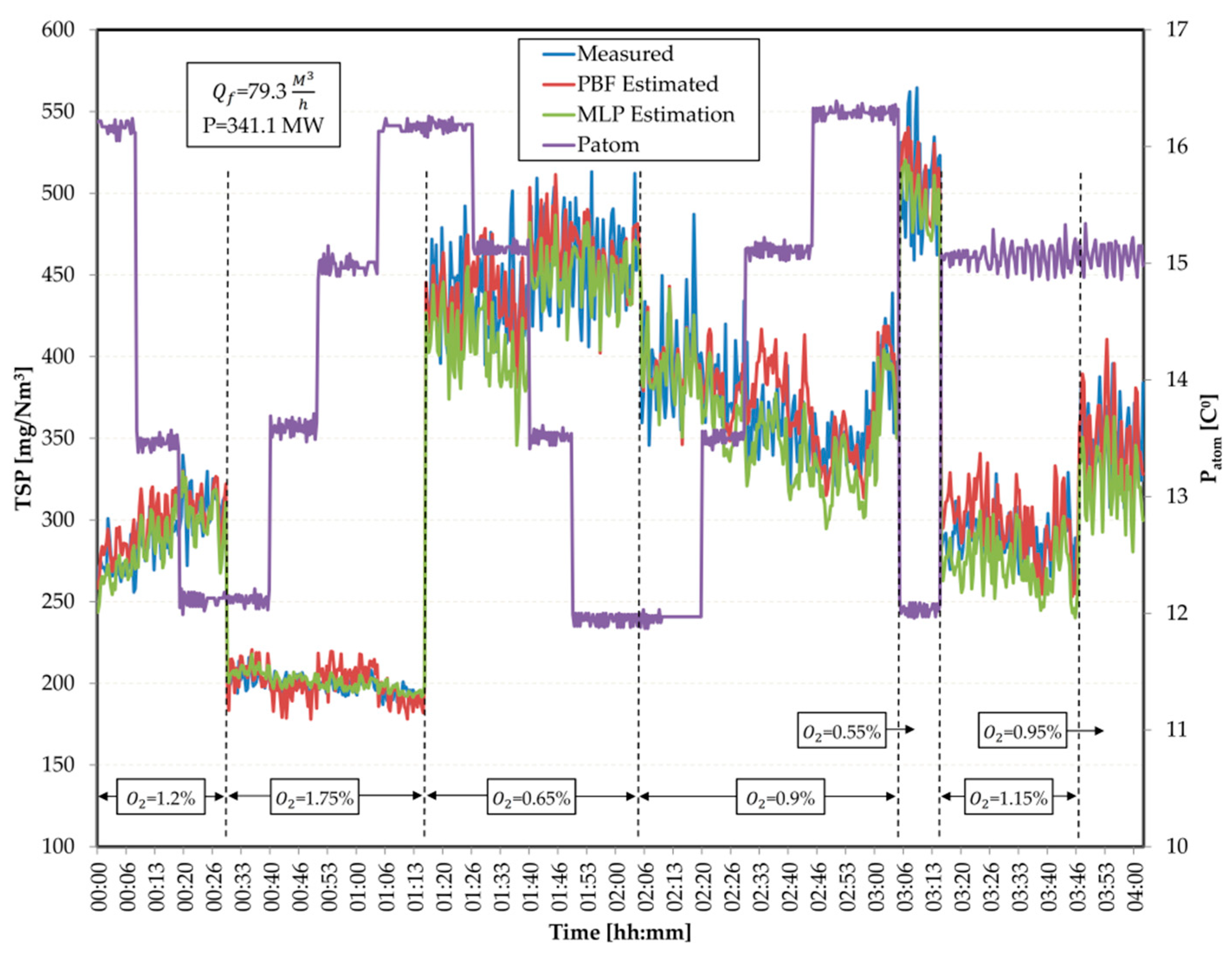
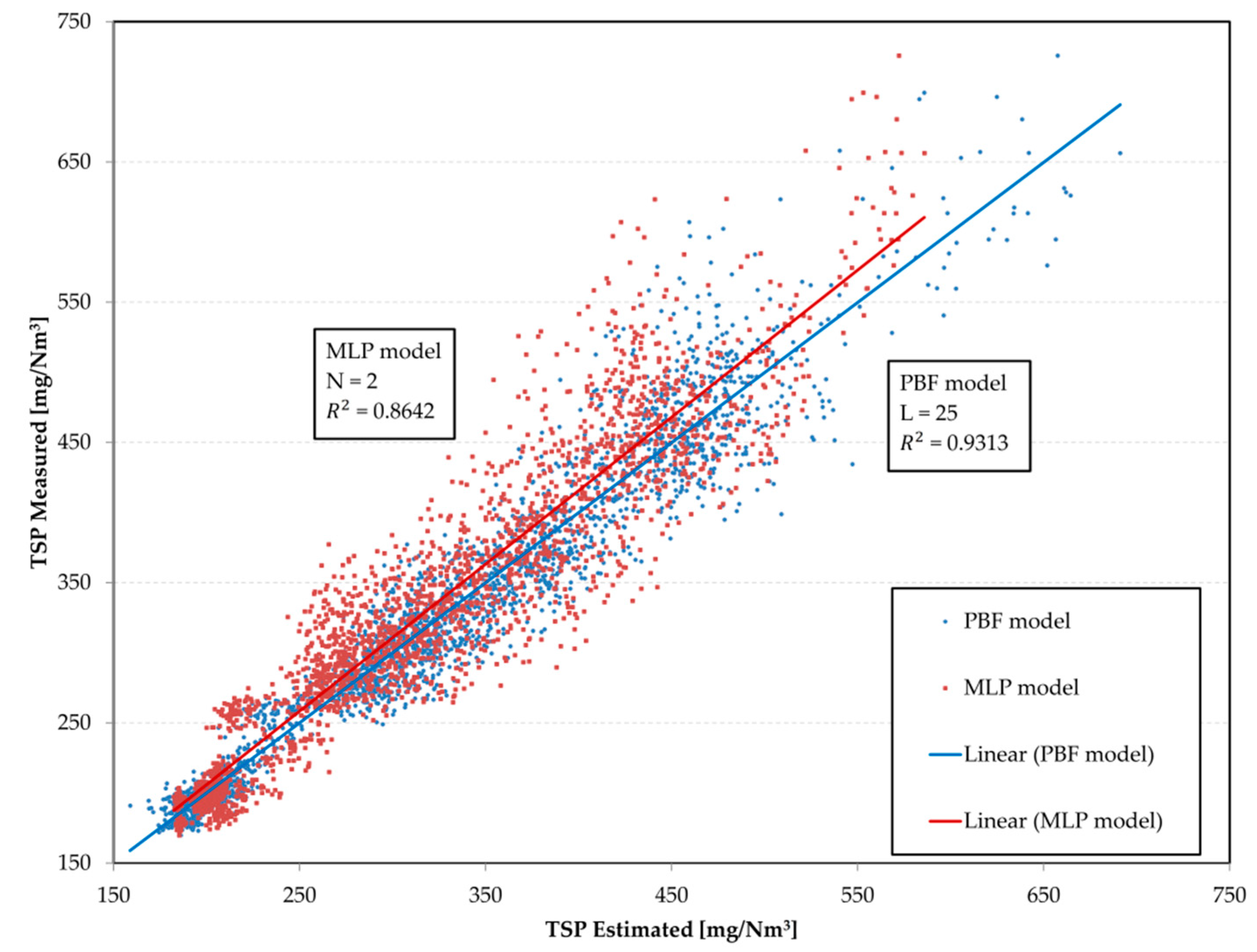
PBF networks provide a viable alternative for the complex multivariable non-linear systems modelling in the industry, where there is little or no process knowledge. The model structure developed allows TSP emissions estimation due to fossil fuel combustion. Non-linear combinations of oxygen excess, atomization pressure, fuel temperature, load, and flow fuel values are sufficiently informative to predict TSP emissions with excellent precision. The TSP emissions estimation can be improved by increasing the training set with experimental tests. The estimation algorithm requires few resources for its implementation, providing a viable alternative for estimating pollutant emissions into the atmosphere during fossil fuel combustion processes.

This methodology can be replicated for other pollutants estimation emitted into the atmosphere in combustion processes, such as, for example, NOx and CO emissions, etc., and has a great application potential, regarding process design, process control combustion optimization, emission control, fault detection, etc., that would bring great benefits in the prevention of diseases, climate change, etc.

References

1. Kumar, P.; Jain, S.; Gurjar, B.R.; Sharma, P.; Khare, M.; Morawska, L.; Britter, R. New Directions: Can a “blue sky” return to Indian megacities? Atmos. Environ. 2013, 71, 198–201. [Google Scholar] [CrossRef] [Green Version]
2. Molina, L.T.; Molina, M.J.; Slott, R.S.; Kolb, C.E.; Gbor, P.K.; Meng, F.; Singh, R.B.; Galvez, O.; Sloan, J.J.; Anderson, W.; et al. Air Quality in Selected Megacities. J. Air Waste Manag. Assoc. 2004, 54, 1–73. [Google Scholar] [CrossRef]
3. Akimoto, H. Global Air Quality and Pollution. Science 2003, 302, 1716–1719. [Google Scholar] [CrossRef] [PubMed] [Green Version]
4. Lim, S.S.; Vos, T.; Flaxman, A.D.; Danaei, G.; Shibuya, K.; Adair-Rohani, H.; Amann, M.; Anderson, H.R.; Andrews, K.G.; Aryee, M.; et al. A comparative risk assessment of burden of disease and injury attributable to 67 risk factors and risk factor clusters in 21 regions, 1990–2010: A systematic analysis for the Global Burden of Disease Study 2010. Lancet 2012, 380, 2224–2260. [Google Scholar] [CrossRef]
5. Sharma, P.; Sharma, P.; Jain, S.; Kumar, P. An integrated statistical approach for evaluating the exceedence of criteria pollutants in the ambient air of megacity Delhi. Atmos. Environ. 2013, 70, 7–17. [Google Scholar] [CrossRef] [Green Version]
6. Kumar, P.; Morawska, L.; Birmili, W.; Paasonen, P.; Hu, M.; Kulmala, M.; Harrison, R.M.; Norford, L.; Britter, R. Ultrafine particles in cities. Environ. Int. 2014, 66, 1–10. [Google Scholar] [CrossRef] [PubMed] [Green Version]
7. White, R.M.; Paprotny, I.; Doering, F.; Cascio, W.E.; Solomon, P.A.; Gundel, L.A. Sensors and “apps” for community-based: Atmospheric monitoring. EM Air Waste Manag. Assoc. Mag. Environ. Manag. 2012, 5, 36–40. [Google Scholar]
8. Kittelson, D.B.; Watts, W.F.; Johnson, J.P. Nanoparticle emissions on Minnesota highways. Atmos. Environ. 2004, 38, 9–19. [Google Scholar] [CrossRef]
9. Heal, M.R.; Kumar, P.; Harrison, R.M. Particles, air quality, policy and health. Chem. Soc. Rev. 2012, 41, 6606–6630. [Google Scholar] [CrossRef] [PubMed] [Green Version]
10. WHO. Ambient (Outdoor) Air Pollution Database by Country and City. United Nations 2014. Available online: http://www.who.int/phe/health_topics/outdoorair/databases/cities-2014/en/ (accessed on 14 June 2018).
11. Medina, S.; Plasencia, A.; Ballester, F.; Mücke, H.G.; Schwartz, J. Apheis: Public health impact of PM10 in 19 European cities. J. Epidemiol. Community Health 2004, 58, 831–836. [Google Scholar] [CrossRef] [PubMed]
12. DEFRA. Automatic Urban and Rural Network (AURN) 2018. Available online: https://uk-air.defra.gov.uk/networks/network-info?view=aurn (accessed on 14 June 2018).
13. Zhu, H.P.; Zhou, Z.Y.; Yang, R.Y.; Yu, A.B. Discrete particle simulation of particulate systems: Theoretical developments. Chem. Eng. Sci. 2007, 62, 3378–3396. [Google Scholar] [CrossRef]
14. Merbitz, H.; Fritz, S.; Schneider, C. Mobile measurements and regression modeling of the spatial particulate matter variability in an urban area. Sci. Total Environ. 2012, 438, 389–403. [Google Scholar] [CrossRef] [PubMed]
15. Aragón, F.M.; Miranda, J.J.; Oliva, P. Particulate matter and labor supply: The role of caregiving and non-linearities. J. Environ. Econ. Manag. 2017, 86, 295–309. [Google Scholar] [CrossRef]
16. Drewnick, F.; Schwab, J.J.; Jayne, J.T.; Canagaratna, M.; Worsnop, D.R.; Demerjian, K.L. Measurement of Ambient Aerosol Composition During the PMTACS-NY 2001 Using an Aerosol Mass Spectrometer. Part I: Mass Concentrations Special Issue of Aerosol Science and Technology on Findings from the Fine Particulate Matter Supersites Program. Aerosol Sci. Technol. 2004, 38, 92–103. [Google Scholar] [CrossRef] [Green Version]
17. Gozzi, F.; Della Ventura, G.; Marcelli, A. Mobile monitoring of particulate matter: State of art and perspectives. Atmos. Pollut. Res. 2016, 7, 228–234. [Google Scholar] [CrossRef]
18. Honarvar, A.R.; Sami, A. Towards Sustainable Smart City by Particulate Matter Prediction Using Urban Big Data, Excluding Expensive Air Pollution Infrastructures. Big Data Res. 2018, 1, 1–10. [Google Scholar] [CrossRef]
19. Soni, M.; Payra, S.; Verma, S. Particulate matter estimation over a semi arid region Jaipur, India using satellite AOD and meteorological parameters. Atmos. Pollut. Res. 2018, 9, 949–958. [Google Scholar] [CrossRef]
20. Vakili, M.; Sabbagh-Yazdi, S.R.; Khosrojerdi, S.; Kalhor, K. Evaluating the effect of particulate matter pollution on estimation of daily global solar radiation using artificial neural network modeling based on meteorological data. J. Clean. Prod. 2017, 141, 1275–1285. [Google Scholar] [CrossRef]
21. Belis, C.A.; Karagulian, F.; Larsen, B.R.; Hopke, P.K. Critical review and meta-analysis of ambient particulate matter source apportionment using receptor models in Europe. Atmos. Environ. 2013, 69, 94–108. [Google Scholar] [CrossRef]
22. Jia, J.; Cheng, S.; Yao, S.; Xu, T.; Zhang, T.; Ma, Y.; Wang, H.; Duan, W. Emission characteristics and chemical components of size-segregated particulate matter in iron and steel industry. Atmos. Environ. 2018, 182, 115–127. [Google Scholar] [CrossRef]
23. Lee, S.W.; Pomalis, R.; Kan, B. A new methodology for source characterization of oil combustion particulate matter. Fuel Process. Technol. 2000, 65–66, 189–202. [Google Scholar] [CrossRef]
24. Ye, H.; Nicolai, R.; Reh, L. A Bayesian–Gaussian neural network and its applications in process engineering. Chem. Eng. Process. 1998, 37, 439–449. [Google Scholar] [CrossRef]
25. Liu, Y.; Peng, C. Time-Variation Nonlinear System Identification Based on Bayesian-Gaussian Neural Network. In Proceedings of the 2009 Fifth International Conference on Natural Computation, Tianjin, China, 14–16 August 2009; pp. 353–357. [Google Scholar] [CrossRef]
26. Chen, S.; Cowan, C.N.; Grant, P.M. Orthogonal least squares learning algorithm for radial basis function networks. IEEE Trans. Neural Netw. 1991, 2, 302–309. [Google Scholar] [CrossRef] [PubMed] [Green Version]
27. Kassam, S.A.; Cha, I. Radial basis function networks in nonlinear signal processing applications. Signals Syst. Comput. 1993, 2, 1021–1025. [Google Scholar]
28. Zeng, X.; Zhao, H.; Jin, W. Nonlinear Plant Identifier Using the Multiple Adaptive RBF Network Convex Combinations. In Advances in Computer Science and Information Engineering; Springer: Berlin/Heidelberg, Germany, 2012; Volume 2, pp. 185–191. [Google Scholar]
29. Liu, G.P. Nonlinear Identification and Control: A Nueral Network Approach; Springer: London, UK; New York, NY, USA, 2001. [Google Scholar]
30. Astrom, K.J.; Wittenmark, B. Computer-Controlled Systems: Theory and Design, 2nd ed.; Prentice Hall International: Upper Saddle River, NJ, USA, 1990. [Google Scholar]
31. Ljung, L. System Identification; Prentice Hall International: Upper Saddle River, NJ, USA, 1998. [Google Scholar]
32. Duda, P.E.; Hart, P.E.; Stork, D.G. Multilayer Neural Networks. In Pattern Classification; Wiley & Sons: Hoboken, NJ, USA, 2000. [Google Scholar]
33. Kohonen, K. Self-Organitation and Asociative Memory, 2nd ed.; Springer: New York, NJ, USA, 1984. [Google Scholar]
34. Powell, M.J.D. Approximation Theory and Methods; Cambridge University Press: Cambridge, UK, 1981. [Google Scholar]
35. Haykin, S. Neural Networks: A Comprehensive Foundation, 2nd ed.; Prentice Hall International: New York, NJ, USA, 1999; Volume 13. [Google Scholar]
36. Billings, S.A.; Chen, S.; Korenberg, M.J. Identification of MIMO non-linear systems using a forward-regression orthogonal estimator. Int. J. Control 1989, 49, 2157–2189. [Google Scholar] [CrossRef] [Green Version]
37. Billings, S.A.; Korenberg, M.J.; Chen, S. Identification of non-linear output-affine systems using an orthogonal least-squares algorithm. Int. J. Syst. Sci. 1988, 19, 1559–1568. [Google Scholar] [CrossRef] [Green Version]
38. Ronquillo-Lomeli, G.; Romero, C.E.; Yao, Z.; Si, F.; Coria-Silva, R.; Hernandez-Rosales, F.; José Sanchez-Gaytana, L.; Trejo-Moralesa, A. On-line flame signal time series analysis for oil-fired burner optimization. Fuel 2015, 158, 416–423. [Google Scholar] [CrossRef]
Figure 1. Identification based on neural networks.
Energies 11 03097 g001
Figure 2. Boiler unit configuration. TSP: total suspended particles, CEMS: continuous emissions monitoring systems, Tf: fuel temperature, Qf: fuel mass flow, Patom: atomization pressure, O2: oxygen excess, FGR: flue gas recirculation, DAS: data acquisition system.
Energies 11 03097 g002
Figure 3. Effect of O2 excess and FGR gate opening level on TSP emissions.
Energies 11 03097 g003
Figure 4. Steam atomization pressure effects on TSP emissions.
Energies 11 03097 g004
Figure 5. Polynomial basis function (PBF)–artificial neural networks (ANN) model structure for TSP modelling.
Energies 11 03097 g005
Figure 6. MLP–ANN model structure for TSP modelling.
Energies 11 03097 g006
Figure 7. Measured (validation subset) and estimated TSP with the PBF and MLP models.
Energies 11 03097 g007
Figure 8. TSP emission models performance.
Energies 11 03097 g008