Cascaded Robust Fault-Tolerant Predictive Control for PMSM Drives

College of Electrical and Information Engineering, Hunan University, Changsha 410082, China
*
Authors to whom correspondence should be addressed.
Energies 2018, 11(11), 3087; https://doi.org/10.3390/en11113087
Submission received: 24 October 2018
/
Revised: 2 November 2018
/
Accepted: 6 November 2018
/
Published: 8 November 2018
Abstract
:This paper presents a cascaded robust fault-tolerant predictive control (CRFTPC) strategy with integral terminal sliding mode observer (IT-SMO) to achieve high performance speed loop and current loop for permanent magnet synchronous motor (PMSM) drives. The modeling of PMSM considers the disturbance caused by parameter perturbation and permanent magnet demagnetization. With this model, we can derive the optimal control law of the proposed scheme, which avoids the tuning work of the weight factor effectively. This new CRFTPC strategy has a cascaded structure, external loop and internal loop, both implemented with robust fault-tolerant predictive control. In addition, a new integral terminal sliding mode observer is designed to estimate the disturbances, and thus the robustness of the proposed method can be increased significantly. Comparative simulations and experimentations verify that the proposed CRFTPC provides fast dynamic response, static-errorless speed, and current tracking, even with the system disturbance.
1. Introduction
Permanent magnet synchronous motor (PMSM) drives based on field oriented control (FOC) have been widely adopted in industrial applications due to the fast and fully decoupled control of torque and flux [1,2,3]. In an FOC-based PMSM drive, the double-loop structure is usually adopted. The internal current loop regulates the stator current to track its reference, while the external speed loop adjusts the machine speed [4]. Thus, the dynamic response and stability of the double-loop are the key factors that determine the dynamic quality of the whole drive system.
A classical approach is based on FOC realized by cascade configuration of the well-known proportional integral (PI) controllers [5]. This approach has been adopted in various application areas, but it also has its limitations. Usually, the parameter settings of the PI controllers only correspond to some specific working ranges. Thus, this causes problems with controllers when the working state of the motor changes [6,7]. In addition, the PMSM control system is a nonlinear system with parameter variations, and permanent magnet demagnetization [8]. In a PMSM, a 20% flux reduction for a ferrite-based magnet creates a 100 °C increase in ambient temperature [9]. Thus, it is difficult for PI control algorithms to achieve a satisfied performance in the entire operating range for PMSM [10,11].
To obtain high performance for PMSM drives control, predictive current control (PCC) approach has been utilized in a wide range of applications. PCC can calculate the required command voltage based on the discrete mathematical model of PMSM, and enable the feedback current to optimally track its reference [12]. Compared with the well-known PI controllers, PCC theoretically improves the dynamic performance of motors [13,14]. However, PCC is absolutely dependent on the exact PMSM model, which means that parameter perturbation and permanent magnet demagnetization would deteriorate the performance of the PCC algorithm.
Some robust PCC methods have been introduced to eliminate the effect of parameter perturbation and demagnetization. In Reference [15], an extension of the PCC method is presented to improve the prediction accuracy for a PMSM. The proposed strategy can not only reduce the current ripple but also improve the robustness of the PCC against parameter uncertainties. In Reference [16], a flux immunity robust predictive control is proposed for PMSM drives, which can operate without knowing the rotor flux. In Reference [17], an improved deadbeat PCC algorithm for the PMSM drive systems is proposed to optimize the current control performance of the PMSM with model parameter mismatch and one-step control delay. In Reference [18], a discrete-time nonlinear robust predictive controller is proposed for the current loop of PMSM drives, which improves the robustness against parametric uncertainties. In References [15,16,17,18], the predictive control performance of the internal current loop has been greatly improved, but a classical PI controller is still used for the external speed loop.
A high-performance servo application must have fast dynamic response, preferably without overshoot, and high steady-state accuracy. Recently, full predictive controls of speed and current of motor drives have been reported [19,20,21,22,23]. In Reference [21], a new speed control strategy for the two-mass system based on the model predictive control scheme is presented. In Reference [22], a control strategy based on finite-set model predictive control for the speed control of the PMSM is developed. In Reference [23], a cascaded predictive speed and current control is proposed based on the explicit inversion of the mechanical model. In References [21,22,23], these methods have some advantages, such as fast transient response and simple implementation. In addition, the sensitive to system parameters and the permanent magnet demagnetization would lead to inaccurate prediction of the motor behavior.
In this paper, the CRFTPC with an integral terminal sliding mode observer is proposed for PMSM drives. The major contributions of this paper are: (1) This work proposes a CRFTPC for the speed and current of PMSM drives, which can avoid the use of the conventional speed PI controller; (2) to improve the robustness of the proposed CRFTPC strategy, a novel integral terminal sliding mode observer is designed for estimating the disturbances; (3) the optimal control law of high performance speed loop and current loop is derived, in which the weighting factor does not need to be introduced. Note that, the proposed speed loop can achieve a satisfied effect during cases of load perturbation and demagnetization. Furthermore, the proposed current loop can effectively enhance robustness against parameter perturbation and demagnetization.
2. Nonlinear Mathematical Model
Machine Model Description
The dq-axis mathematical model of the PMSM can be given as the dq-axis set of the three-phase motor. Thus, the Park and Clarke transformation of dq-axis voltage can be expressed as
where and are the d- and q-axis stator voltages, respectively. , and denote the three phase stator voltage, and is the electrical rotor angle.
The voltage equations of PMSM in synchronous rotating frame are usually described as [24],
Under control, the electromagnetic torque is,
The mechanical dynamic model can be described as follows,
where and are the d- and q-axis currents, respectively; , , and are the nominal value of stator resistance, the d-axis inductance, the q-axis inductance and the moment of inertia, respectively. is the friction coefficient, and is the electrical rotor speed. is the flux linkage established by the permanent magnets. is the number of pole pairs, is the electromagnetic torque, and is the load torque.
During the operation of the PMSM, motor parameter perturbation and permanent magnet demagnetization occur due to the influence of temperature. Introducing ,, and , where , and are nominal values and , and are perturbation values of the corresponding model parameters. The flux linkage amplitude varies from initial to , when demagnetization fault occurs, and defining as the new flux linkage components of d-axis. Therefore, the voltage equations are expressed as follows,
where and represent the unknown disturbances caused by parameter perturbation and demagnetization, that can be defined as
When permanent magnet demagnetization occurs, the electromagnetic torque produced by the machine is
The mechanical dynamics of the PMSM model is then
where represents unknown external disturbances. is the unknown load disturbance caused by permanent magnet demagnetization.
According to Equations (5), (7) and (8), the nonlinear mathematical model of PMSM can be established
where , , , and are state variables, system inputs, system outputs, and unknown disturbances. The coefficient matrixes of the state equations are
3. Disturbances Analysis
3.1. Effect of Disturbance on Speed Loop
When the PI controller is used, the block diagram of the speed loop control system under permanent magnet demagnetization is shown in Figure 1.
According to Figure 1, the transfer function between and can be obtained as follows:
where and separately represent the proportional and integral coefficients, that are set to 2000 and 0.5.
The motor parameters are shown in Table 1. According to Equation (10), the amplitude characteristics with different values are plotted in the Bode diagram of Figure 2. As shown in Figure 2, the effect of on the PMSM speed loop control is very strong. Therefore, the effect of permanent magnet demagnetization on speed control cannot be ignored. The conventional PI controller cannot satisfy the requirements of control precision.
3.2. Effect of Disturbance on Current Loop
According to Equation (5), the stationary equations are given as below [25]:
The control strategy is mainly studied in this paper. Thus, compared with the q-axis current, the function of the d-axis current can be basically ignored. Combining with Equation (11), the d- and q-axis disturbance can be simplified as follows:
The motor parameters are shown in Table 1. According to Equation (12), the d-and q-axis disturbance can be plotted, as shown in Figure 3. Figure 3a shows the d- and q-axis disturbance under resistance parameter perturbation. The d-axis disturbance is zero, and the q-axis disturbance is negative. Figure 3a illustrates that the resistance parameter perturbation does not affect the d-axis current, and the influence of resistance parameters perturbation can be neglected according to the influence of inductance and flux linkage parameters on the q-axis current. Figure 3b shows the d- and q-axis disturbance under inductance parameter perturbation. The q-axis disturbance is zero. The d-axis disturbance is positive, and increases with the raise of the speed and torque. Figure 3b illustrates that the inductance parameter perturbation does not affect the q-axis current, but seriously affect the d-axis current. Figure 3c shows the d- and q-axis disturbance under permanent magnet demagnetization. The d-axis disturbance is zero. The q-axis disturbance is negative, and increases with the growing of the speed. Figure 3c illustrates that the permanent magnet demagnetization does not affect the d-axis current, but has strong influence on the q-axis current. From the above analysis, we can observe that the inductance and flux parameters have great influence on the performance of the control system, whereas the effect of the resistance parameters can be neglected.
4. Design of the CRFTPC
4.1. Design of the Optimal Control Law
The predictive output and reference output are separately defined as
To simplify the calculations, the predicted output and the reference output are expanded into 1st order Taylor series as
where
The selection of the cost function reflects the requirements of the control system performance. Servo control belongs to the tracking control system, and it expects that the controlled output will track the reference input at the fastest speed. To improve the dynamic response of the predictive control performance, the optimal control law in this paper is calculated in half the sampling period. The block diagram of the conventional predictive control method is illustrated in Figure 4a. The block diagram of the proposed CRFTPC method is illustrated in Figure 4b.
Thus, the cost function is defined as
where is the sampling period.
With
where .
Substituting Equations (14) into (13), the cost function can be expressed as
where , , , .
The necessary condition for the optimal control law is given by
Substituting Equations (15) into (16), we can obtain
Thus, the optimal control law can be obtained according to Equation (17).
To enhance the robustness of the predictive control system, the IT-SMO is designed to observe the external disturbances. The disturbance observer value is used as the feedback input of the predictive control system. According to Equation (18), the optimal control law can be expressed as
where are the observed values of .
4.2. Stability Analysis
According to Equation (19), The error equation of the predictive closed-loop system can be expressed as follows:
where .
In Section 5, when the proposed IT-SMO is convergent, where , then . The Lyapunov function is defined as
Differentiating the Lyapunov function (Equation (21)), it yields
From Equation (22), the predictive closed-loop system is locally asymptotically stable. This completes the proof.
4.3. Design of Predictive Speed Controller
The predictive speed controller is used to realize the speed control in this paper. The IT-SMO is designed to observe the external disturbance, so as to improve the robustness against the load perturbation and permanent magnet demagnetization.
According to Equation (19), the predictive speed controller can be designed as follows:
where is the observed value of . is the q-axis current reference output by the predictive speed controller.
4.4. Design of Predictive Current Controller
The main objective of the current control is to efficiently control motor currents with high accuracy. Parameter perturbation and permanent magnet demagnetization will deteriorate the current control performance if these factors are not considered in the design of the controller.
According to Equation (19), the predictive speed controller can be designed as follows:
where , are the observed values of , , , are the d- and q-axis voltage reference outputs by the predictive current controller. The block diagram of the two model predictive control (MPC) implementations are shown in Figure 5. The block diagram of the PMSM drive system with CRFTPC method is shown in Figure 6.
4.5. Design of IT-SMO
According to Equation (9), the IT-SMO can be designed as follows:
where is the observed value of ; is the sliding mode control function.
Considering the following integral terminal sliding surfaces vector,
where , , is the sign function; the is defined as follows:
In practical applications, chattering suppression is important to design observers since the chattering of the sign function can easily result in the chattering of the system. For this purpose, the sign function is replaced with a hyperbolic tangent function with a smooth continuity. The hyperbolic tangent function can be expressed as [26,27]
Taking a time derivative from Equation (26), and combining Equations (25) with (10), the error equation of the TI-SMO can be obtained:
where is a positive diagonal matrix, is the observer sliding gain.
Theorem 1.
Consider the integral terminal sliding surface (Equation (26)) with the error Equation (28). When the sliding mode control function of Equation (29) is designed, the error convergence can be guaranteed.
Consider the following Lyapunov function candidate
Differentiating the Lyapunov function (Equation (30)) and combining the obtained result with the result in Equation (29) yields
By applying the sliding mode control function (Equation (29)), it yields
where .
According to an engineering point of view, the disturbances should be bounded, that is, there exists a normal value satisfying . According to Equation (32), if satisfies the condition of , where , then .
Therefore, the stability and convergence of the IT-SMO is guaranteed based on the sliding-mode control theory. This completes the proof.
According to the sliding mode equivalent principle, when the system reaches the sliding-mode surface that is , then the error equation (Equation (28)) can be simplified as follows:
From Equation (33), the estimated disturbances can be represented as:
5. Simulations
Simulations are established in MATLAB/Simulink, the DC voltage is 1500 V, and the amplitude value of the stator current is 350 A. The proposed IT-SMO parameters are , and . To realize the inductance parameter perturbation and permanent magnet demagnetization in MATLAB/Simulink, according to Equation (5), we reconstruct the PMSM module by using the step module to simulate the inductance parameter perturbation and permanent magnet demagnetization. The main parameters of the PMSM used in the simulation and experiment are shown in Table 1.
5.1. Speed Control Performance Comparison of Conventional PI and Proposed CRFTPC
In Figure 7 and Figure 8, the control precision of the proposed CRFTPC is directly compared with that of the conventional PI controller under the same conditions. Figure 7 shows the comparison of the two controllers against step change of the load torque. At 4 and 6 s, the load torque is increased suddenly from 300 to 700 N and decreased from 700 to 300 N, respectively. Figure 8 shows the comparison of the two controllers against step change of the flux linkage. At 4 and 6 s, the flux linkage is decreased suddenly from 0.892 to 0.446 Wb and increased from 0.446 to 0.892 Wb, respectively. The results show that when the load perturbation and permanent magnet demagnetization occur, the proposed IT-SMO can accurately estimate disturbance. Moreover, the control precision of the proposed scheme is obviously better than that of a PI controller during cases of load perturbation and permanent magnet demagnetization.
5.2. Current Control Performance Comparison of Conventional PCC and Proposed CRFTPC
In Figure 9 and Figure 10, the current control performance of the proposed CRFTPC is directly compared with that of the conventional PCC controller under the same conditions. At 4 and 6 s, the load torque is increased suddenly from 300 to 600 N and decreased from 600 to 300 N, respectively. Figure 9 and Figure 10 show the comparison of the two controllers against inductance parameter perturbation and permanent magnet demagnetization, respectively. The results show that the proposed IT-SMO can accurately estimate disturbance caused by inductance parameter perturbation and permanent magnet demagnetization. Furthermore, we observe that inductance parameter perturbation and permanent magnet demagnetization have an effect on current responses in the conventional PCC method. However, current responses track their references accurately using the proposed CRFTPC. As expected, the response time of the proposed CRFTPC is obviously shorter than that of a conventional PCC controller, which means that the dynamic response of the proposed CRFTPC is faster than that of a conventional PCC controller.
6. Experiments
To validate the control strategy, a 10 kW interior permanent magnet synchronous motor (IPMSM) prototype was established, as shown in Figure 11. The 12 kVA active front-end is a DC-DC converter, linked the DC source to realize the modification of the DC-link voltage. The per-unit (p.u.) values of 10 kW PMSM parameters were consistent with those of the simulation model.
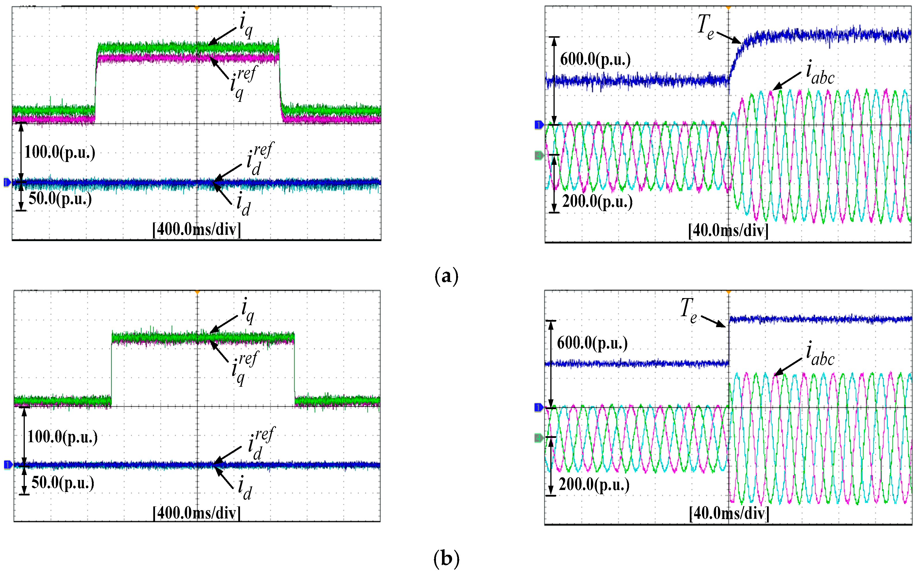
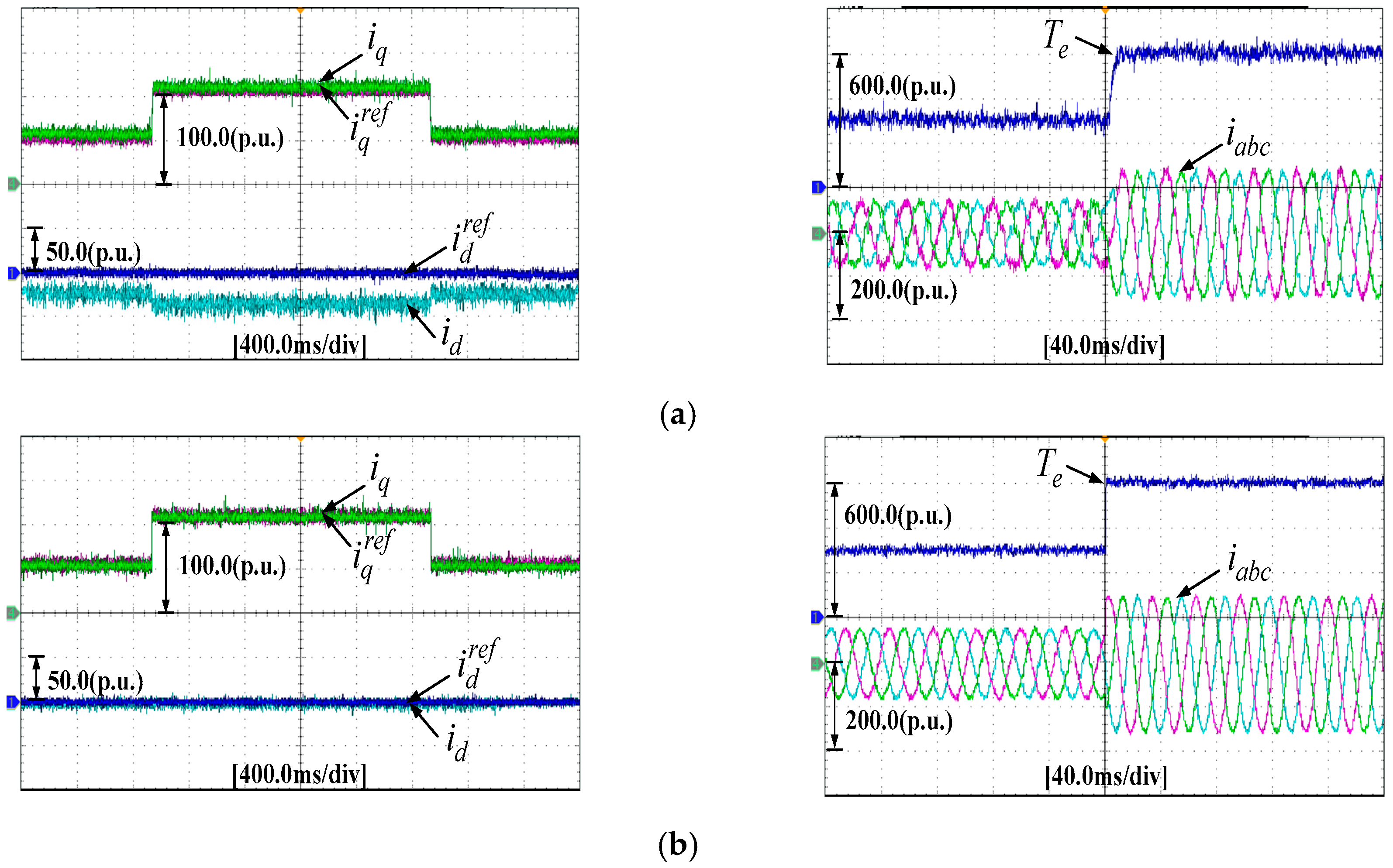
In Figure 12 and Figure 13, the experimental results of the conventional PI and CRFTPC under the condition of load perturbation and permanent magnet demagnetization are shown. The experimental results show that load perturbation and permanent magnet demagnetization have the effects on the speed of the conventional PI controller. By contrast, these results show that CRFTPC has better disturbance rejection ability due to disturbance compensation. Figure 14 and Figure 15 show the control performance comparisons of the conventional PCC and CRFTPC under inductance parameter perturbation and permanent magnet demagnetization. The experimental results indicate that the CRFTPC method exhibits a faster response time than the conventional PCC under inductance parameter perturbation and permanent magnet demagnetization. Moreover, it can be seen that the CRFTPC method can efficiently track current references with high accuracy. In conclusion, the CRFTPC results demonstrate that the currents and torque remain stable and behave with excellent dynamic and steady performance, in spite of the inductance parameter perturbation and permanent magnet demagnetization.
7. Conclusions
In this paper, a CRFTPC strategy based on IT-SMO for the speed and current control of the PMSM, without the conventional speed PI controller, has been developed. The proposed CRFTPC can achieve fast dynamic response, which is very important for high-performance FOC-based PMSM drives. The steady-state current tracking error caused by parameter perturbation and permanent magnet demagnetization is eliminated by introducing the disturbance term into the proposed control law. Moreover, the proposed CRFTPC can effectively guarantee the control precision of the speed loop regardless of load perturbation and permanent magnet demagnetization.
The proposed scheme has been verified through simulations and experimental tests, and the results are satisfactory. Compared with the conventional speed PI controller, the proposed scheme shows its superiority in control precision and disturbance rejection. In addition, the proposed scheme successfully overcame the conventional PCC weaknesses by presenting strong robustness and excellent dynamic response in cases of parameter perturbation and permanent magnet demagnetization.
Author Contributions
F.H. and D.L. designed the proposed control strategy, F.H. and D.L. conducted experimental works, modeling and FEA simulation, C.L., Z.L. and G.W. gave help of paper writing.
Funding
This work was supported in part by the National Natural Science Foundation of China (51577052).
Conflicts of Interest
The authors declare no conflicts of interest.
References
- Consoli, A.; Scarcella, G.; Testa, A. Slip-frequency detection for indirect field-oriented control drives. IEEE Trans. Ind. Electron. 2004, 40, 194–201. [Google Scholar] [CrossRef]
- Qian, W.; Panda, S.K.; Xu, J.X. Torque ripple minimization in PM synchronous motors using iterative learning control. IEEE Trans. Power Electron. 2004, 19, 272–279. [Google Scholar] [CrossRef]
- Wang, B.; Chen, X.; Yu, Y.; Wang, G.; Xu, D. Robust predictive current control with online disturbance estimation for induction machine drives. IEEE Trans. Power Electron. 2017, 32, 4663–4674. [Google Scholar] [CrossRef]
- Stojic, D.M.; Milinkovic, M.; Veinovic, S.; Klasnic, I. Stationary frame induction motor feed forward current controller with back EMF compensation. IEEE Trans. Power Electron. 2015, 30, 1356–1366. [Google Scholar] [CrossRef]
- Guzman, H.; Duran, M.J.; Barrero, F.; Zarri, L.; Bogado, B.; Prieto, I.G.; Arahal, M.R. Comparative study of predictive and resonant controllers in fault-tolerant five-phase induction motor drives. IEEE Trans. Ind. Electron. 2016, 63, 606–617. [Google Scholar] [CrossRef]
- Belda, K.; Vošmik, D. Explicit generalized predictive control of speed and position of PMSM drives. IEEE Trans. Ind. Electron. 2016, 63, 3889–3896. [Google Scholar] [CrossRef]
- Bazaz, M.A.; Nabi, M.; Janardhanan, S. Modelling and simulation strategy for parametric transient electromagnetic simulations. Int. J. Model. Identif. Control 2013, 18, 251–260. [Google Scholar] [CrossRef]
- Zhu, M.; Hu, W.; Kar, N.C. Torque-ripple-based interior permanent-magnet synchronous machine rotor demagnetization fault detection and current regulation. IEEE Trans. Ind. Appl. 2017, 53, 2795–2804. [Google Scholar] [CrossRef]
- Ahn, H.J.; Lee, D.M. A new bumpless rotor-flux position estimation scheme for vector-controlled washing machine. IEEE Trans. Ind. Inf. 2016, 12, 466–473. [Google Scholar] [CrossRef]
- Li, S.; Liu, Z. Adaptive speed control for permanent-magnet synchronous motor system with variations of load inertia. IEEE Trans. Ind. Electron. 2009, 56, 3050–3059. [Google Scholar]
- Mercorelli, P.; Lehmann, K.; Liu, S. Robust flatness based control of an electromagnetic linear actuator using adaptive PID controller. In Proceedings of the 42nd IEEE Conference on Decision and Control, Maui, HI, USA, 9–12 December 2003; pp. 3790–3795. [Google Scholar]
- Carpiuc, S.-C.; Lazar, C. Fast real-time constrained predictive current control in permanent magnet synchronous machine-based automotive traction drives. IEEE Trans. Transp. Electrif. 2015, 1, 326–335. [Google Scholar] [CrossRef]
- Cortes, P.; Rodriguez, J.; Silva, C.; Flores, A. Delay compensation in model predictive current control of a three-phase inverter. IEEE Trans. Ind. Electron. 2012, 59, 1323–1325. [Google Scholar] [CrossRef]
- Lim, C.S.; Levi, E.; Jones, M.; Rahim, N.A.; Hew, W.P. FCSMPC-based current control of a five-phase induction motor and its comparison with PI-PWM control. IEEE Trans. Ind. Electron. 2014, 61, 149–163. [Google Scholar] [CrossRef]
- Siami, M.; Khaburi, D.A.; Abbaszadeh, A.; Rodríguez, J. Robustness improvement of predictive current control using prediction error correction for permanent-magnet synchronous machines. IEEE Trans. Ind. Electron. 2016, 63, 3458–3466. [Google Scholar] [CrossRef]
- Yang, M.; Lang, X.; Long, J.; Xu, D. A flux immunity robust predictive current control with incremental model and extended state observer for PMSM drive. IEEE Trans. Power Electron. 2017. [Google Scholar] [CrossRef]
- Zhang, X.; Hou, B.; Yang, M. Deadbeat predictive current control of permanent-magnet synchronous motors with stator current and disturbance observer. IEEE Trans. Power Electron. 2017, 32, 3818–3834. [Google Scholar] [CrossRef]
- Türker, T.; Buyukkeles, U.; Bakan, A.F. A robust predictive current controller for PMSM drives. IEEE Trans. Ind. Electron. 2016, 63, 3906–3914. [Google Scholar] [CrossRef]
- Chai, S.; Wang, L.; Rogers, E. A cascade MPC control structure for a PMSM with speed ripple minimization. IEEE Trans. Ind. Electron. 2013, 60, 2978–2987. [Google Scholar] [CrossRef]
- Sawma, J.; Khatounian, F.; Monmasson, E.; Idkhajine, L.; Ghosn, R. Cascaded dual-model-predictive control of an active front-end rectifier. IEEE Trans. Ind. Electron. 2016, 63, 4604–4614. [Google Scholar] [CrossRef]
- Fuentes, E.J.; Silva, C.A.; Yuz, J.I. predictive speed control of a two-mass system driven by a permanent magnet synchronous motor. IEEE Trans. Ind. Electron. 2012, 59, 2840–2848. [Google Scholar] [CrossRef]
- Fuentes, E.; Kalise, D.; Rodriguez, J.; Kennel, R.M. Cascade-free predictive speed control for electrical drives. IEEE Trans. Ind. Electron. 2014, 61, 2176–2184. [Google Scholar] [CrossRef]
- Garcia, C.; Rodriguez, J.; Silva, C.; Rojas, C.; Zanchetta, P.; Abu-Rub, H. Full predictive cascaded speed and current control of an induction machine. IEEE Trans. Energy Convers. 2016, 31, 1059–1067. [Google Scholar] [CrossRef]
- Alexandrou, A.D.; Adamopoulos, N.K.; Kladas, A.G. Development of a constant switching frequency deadbeat predictive control technique for field-oriented synchronous permanent-magnet motor drive. IEEE Trans. Ind. Electron. 2016, 63, 5167–5175. [Google Scholar] [CrossRef]
- Richter, J.; Doppelbauer, M. Predictive trajectory control of permanent-magnet synchronous machines with nonlinear magnetics. IEEE Trans. Ind. Electron. 2016, 63, 3915–3924. [Google Scholar] [CrossRef]
- Rahman, M.A.; Zhou, P. Analysis of brushless permanent magnet synchronous motors. IEEE Trans. Ind. Electron. 1996, 43, 256–267. [Google Scholar] [CrossRef]
- Mercorelli, P. Parameters identification in a permanent magnet three-phase synchronous motor of a city-bus for an intelligent drive assistant. Int. J. Model. Identif. Control 2014, 21, 352–361. [Google Scholar] [CrossRef]
Figure 1.
Block diagram of PMSM speed loop control.
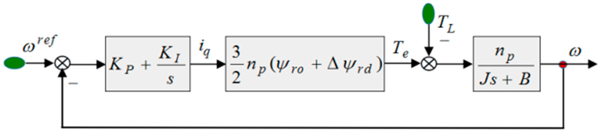
Figure 2.
Variation bode diagram of to .

Figure 3.
d-and q-axis disturbance: (a) resistance parameter perturbation; (b) inductance parameter perturbation and (c) permanent magnet demagnetization.
Figure 3.
d-and q-axis disturbance: (a) resistance parameter perturbation; (b) inductance parameter perturbation and (c) permanent magnet demagnetization.

Figure 4.
(a) Time diagram of conventional predictive control method implementation; (b) time diagram of CRFTPC method implementation.
Figure 4.
(a) Time diagram of conventional predictive control method implementation; (b) time diagram of CRFTPC method implementation.

Figure 5.
The block diagram of CRFTPC method.
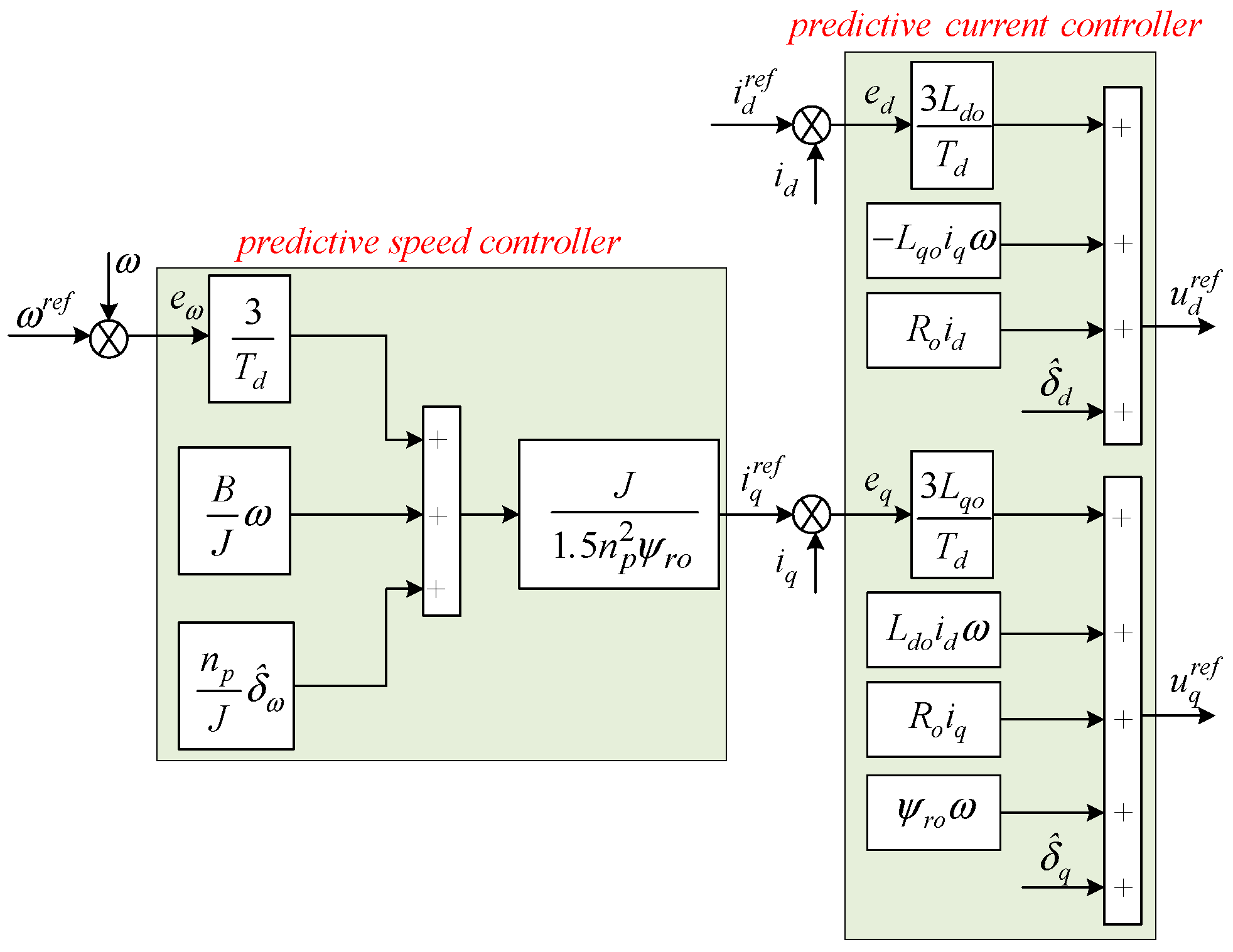
Figure 6.
The block diagram of CRFTPC method with IT-SMO for PMSM.
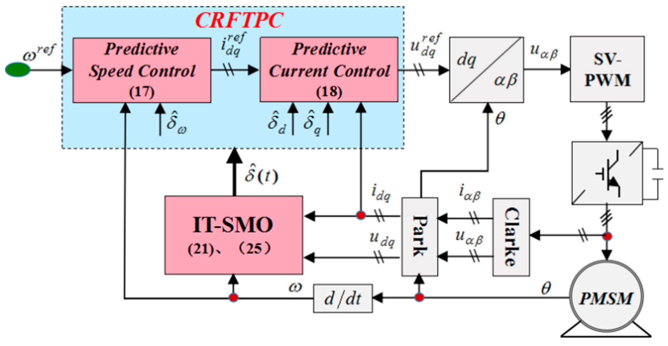
Figure 7.
Simulation comparisons of the two controllers against step change of the load torque: (a) Conventional PI and (b) proposed CRFTPC.
Figure 7.
Simulation comparisons of the two controllers against step change of the load torque: (a) Conventional PI and (b) proposed CRFTPC.
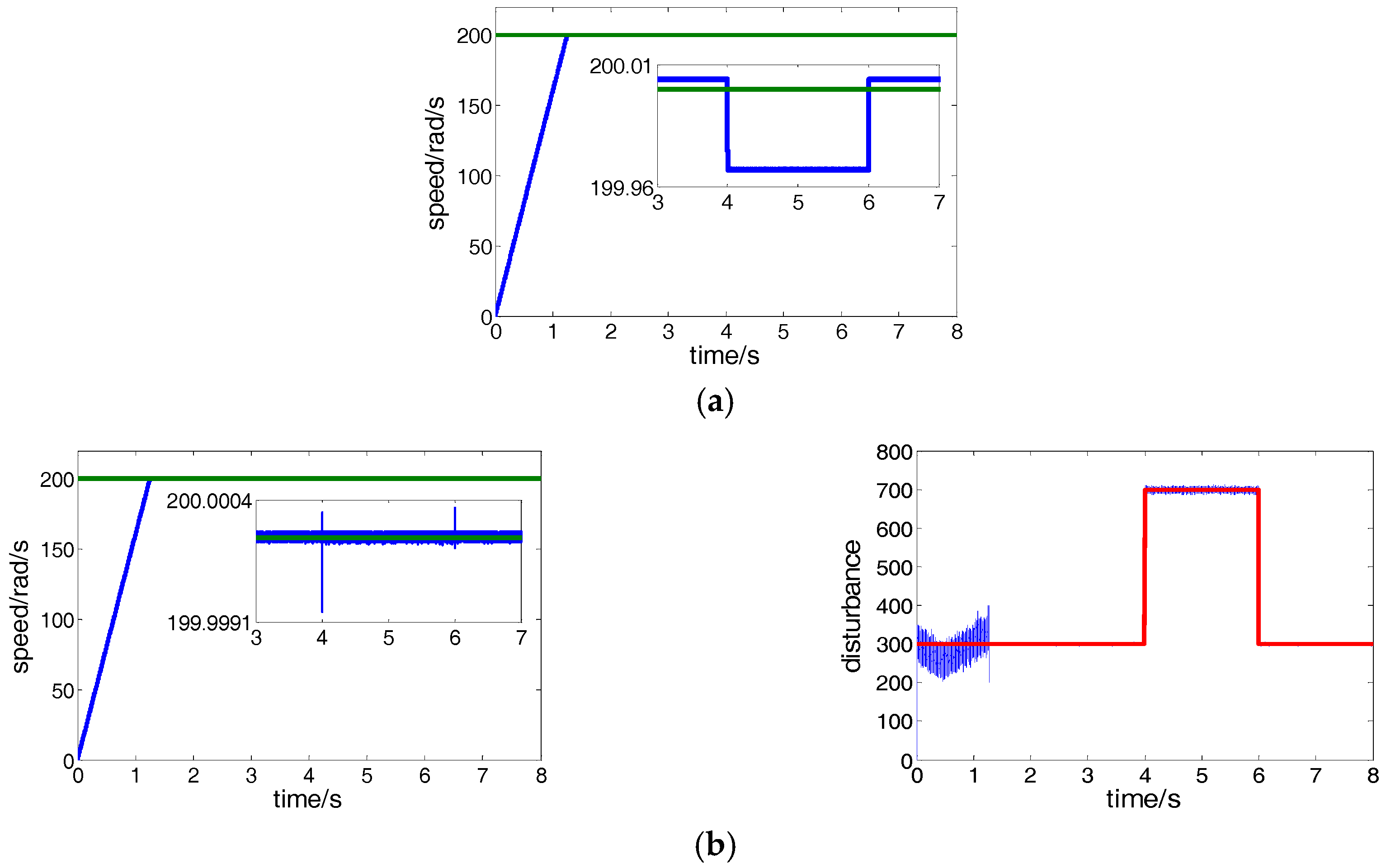
Figure 8.
Simulation comparisons of the two controllers against step change of the flux linkage: (a) Conventional PI and (b) proposed CRFTPC.
Figure 8.
Simulation comparisons of the two controllers against step change of the flux linkage: (a) Conventional PI and (b) proposed CRFTPC.
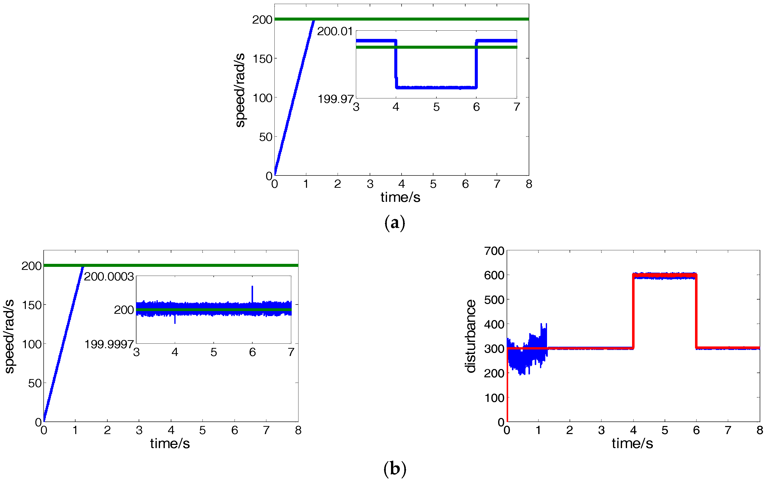
Figure 9.
Simulation comparisons of the two controllers against inductance parameter perturbation (, ): (a) Conventional PCC and (b) proposed CRFTPC.
Figure 9.
Simulation comparisons of the two controllers against inductance parameter perturbation (, ): (a) Conventional PCC and (b) proposed CRFTPC.
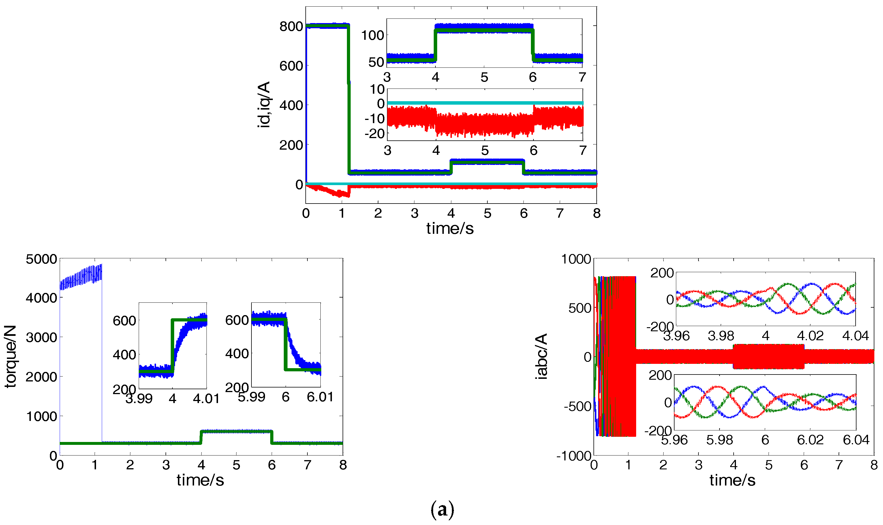
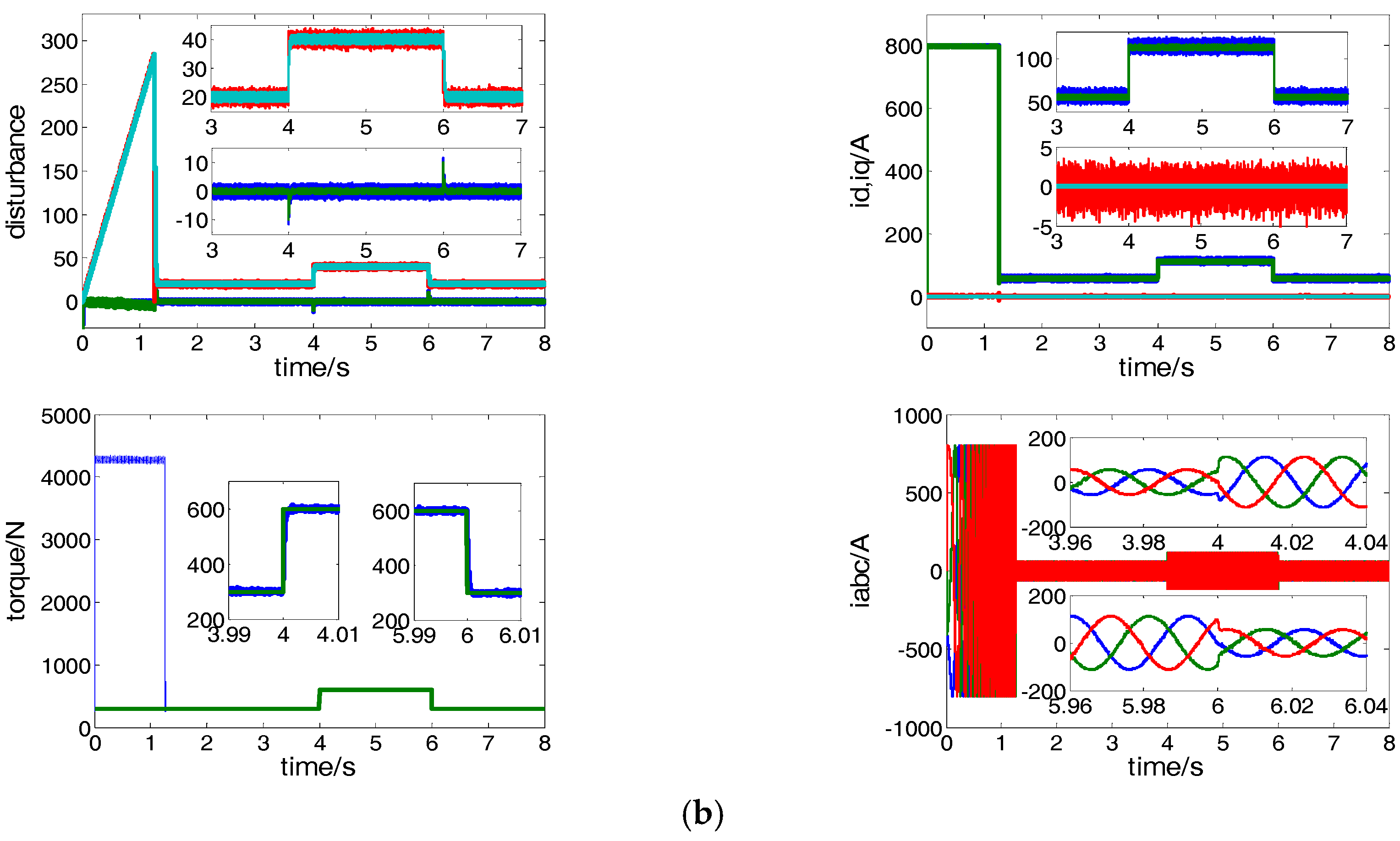
Figure 10.
Simulation comparisons of the two controllers against permanent magnet demagnetization : (a) Conventional PCC and (b) proposed CRFTPC.
Figure 10.
Simulation comparisons of the two controllers against permanent magnet demagnetization : (a) Conventional PCC and (b) proposed CRFTPC.
Figure 11.
Experimental platform of IPMSM drive.
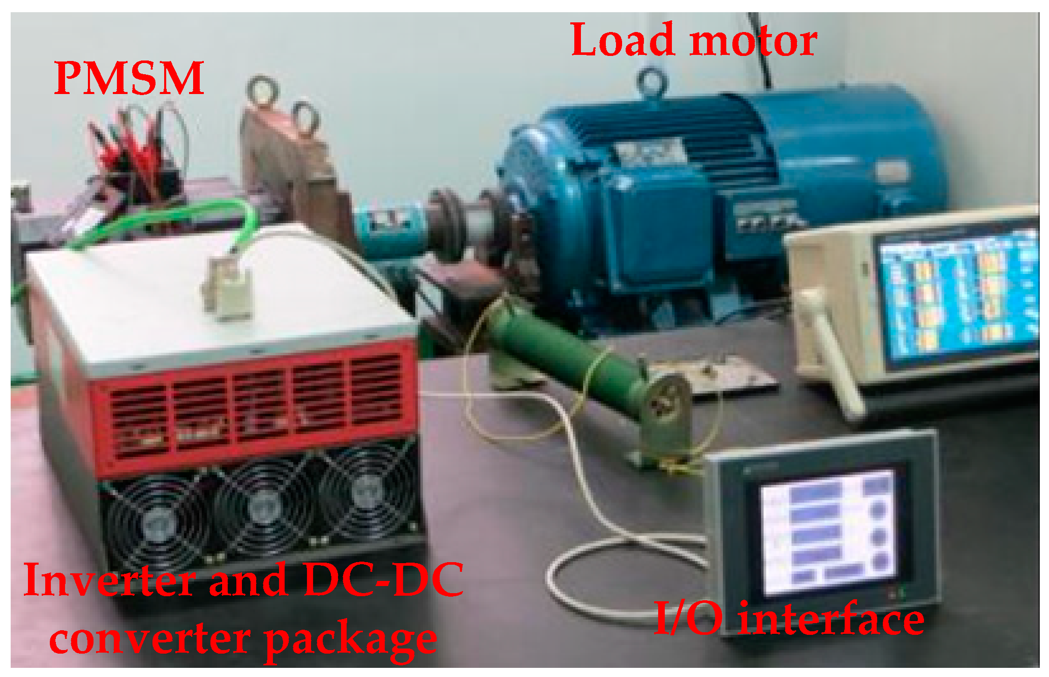
Figure 12.
Experimental comparison of the two controllers against step change of the load torque. (a) Conventional PI and (b) proposed CRFTPC.
Figure 12.
Experimental comparison of the two controllers against step change of the load torque. (a) Conventional PI and (b) proposed CRFTPC.
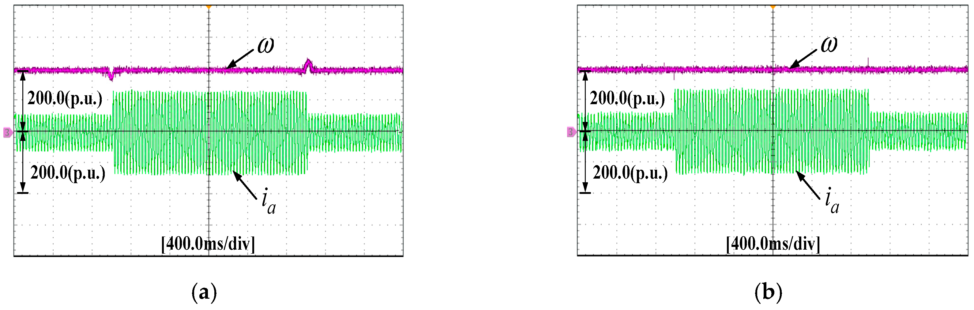
Figure 13.
Experimental comparison of the two controllers against step change of the flux linkage: (a) Conventional PI and (b) proposed CRFTPC.
Figure 13.
Experimental comparison of the two controllers against step change of the flux linkage: (a) Conventional PI and (b) proposed CRFTPC.
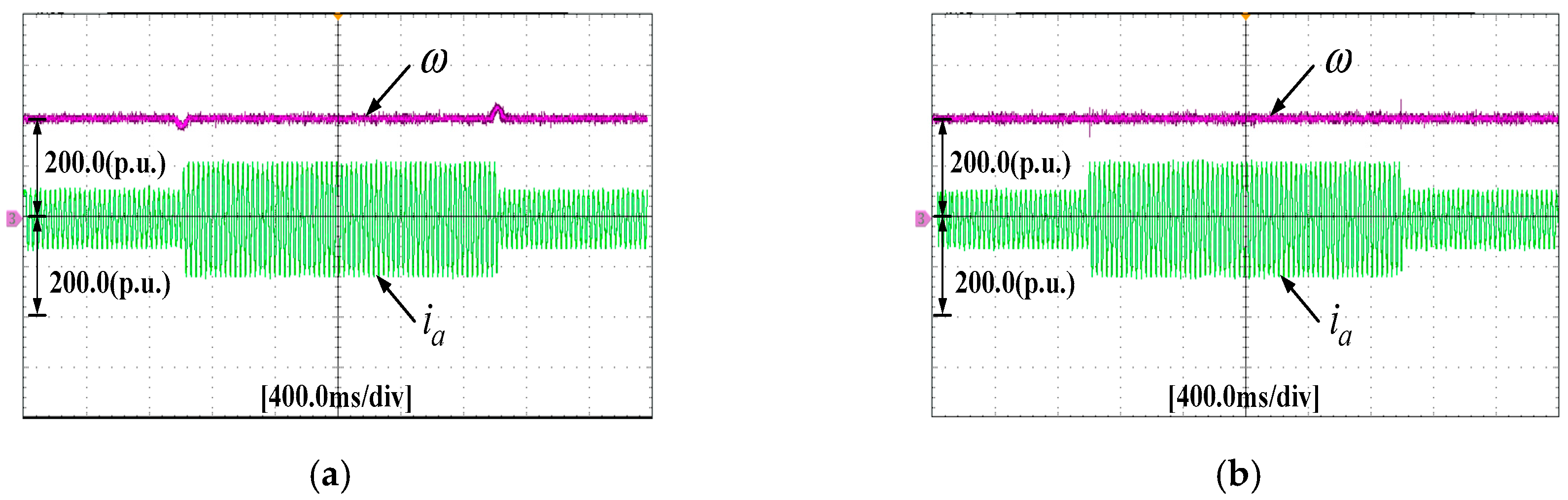
Figure 14.
Experimental comparison of the two controllers against inductance parameter perturbation (, ): (a) Conventional PCC and (b) proposed CRFTPC.
Figure 14.
Experimental comparison of the two controllers against inductance parameter perturbation (, ): (a) Conventional PCC and (b) proposed CRFTPC.

Figure 15.
Experimental comparison of the two controllers against permanent magnet demagnetization : (a) Conventional PCC and (b) proposed CRFTPC.
Figure 15.
Experimental comparison of the two controllers against permanent magnet demagnetization : (a) Conventional PCC and (b) proposed CRFTPC.

Table 1.
Main parameters of PMSM.
| Parameters | Value |
|---|---|
| Stator phase resistance (Ro) | 0.02 Ω |
| Number of pole pairs (np) | 4 |
| d-axis inductances (Ldo) | 0.001 H |
| q-axis inductances (Lqo) | 0.003572 H |
| Flux linkage of permanent magnets (Ψro) | 0.892 Wb |
| Rotational inertia (J) | 100 kg·m2 |
| viscous friction coef (B) | 0.01 kg m2 s−1 |
© 2018 by the authors. Licensee MDPI, Basel, Switzerland. This article is an open access article distributed under the terms and conditions of the Creative Commons Attribution (CC BY) license (http://creativecommons.org/licenses/by/4.0/).
Share and Cite
MDPI and ACS Style
Hu, F.; Luo, D.; Luo, C.; Long, Z.; Wu, G. Cascaded Robust Fault-Tolerant Predictive Control for PMSM Drives. Energies 2018, 11, 3087. https://doi.org/10.3390/en11113087
AMA Style
Hu F, Luo D, Luo C, Long Z, Wu G. Cascaded Robust Fault-Tolerant Predictive Control for PMSM Drives. Energies. 2018; 11(11):3087. https://doi.org/10.3390/en11113087
Chicago/Turabian StyleHu, Fang, Derong Luo, Chengwei Luo, Zhuo Long, and Gongping Wu. 2018. "Cascaded Robust Fault-Tolerant Predictive Control for PMSM Drives" Energies 11, no. 11: 3087. https://doi.org/10.3390/en11113087
Note that from the first issue of 2016, this journal uses article numbers instead of page numbers. See further details here.