Article

Wind Turbulence Intensity at La Ventosa, Mexico: A Comparative Study with the IEC61400 Standards

by
C. A. Lopez-Villalobos
1,*,†,
O. Rodriguez-Hernandez
2,†,
R. Campos-Amezcua
3,†,
Guillermo Hernandez-Cruz
2,
O. A. Jaramillo
2 and
J. L. Mendoza
4
1
Posgrado en Ingeniería, Universidad Nacional Autonoma de Mexico, Priv. Xochicalco s/n, Col. Centro, Temixco, Morelos CP 62580, Mexico
2
Instituto de Energías Renovables, Universidad Nacional Autonoma de Mexico, Priv. Xochicalco s/n, Col. Centro, Temixco, Morelos CP 62580, Mexico
3
Tecnológico Nacional de México, Instituto Tecnológico de La Laguna, Blvd. Revolución y Av. Instituto Tecnológico de La laguna s/n, Centro, Torreón 27000, Coahuila, Mexico
4
Instituto Nacional de Electricidad y Energías Limpias (INEEL), Cuernavaca, Morelos CP 62580, Mexico
*
Author to whom correspondence should be addressed.
These authors contributed equally to this work.
Energies 2018, 11(11), 3007; https://doi.org/10.3390/en11113007
Submission received: 18 September 2018 / Revised: 26 October 2018 / Accepted: 27 October 2018 / Published: 1 November 2018

Abstract

:
Wind speed turbulence intensity is a crucial parameter in designing the structure of wind turbines. The IEC61400 considers the Normal Turbulence Model (NTM) as a reference for fatigue load calculations for small and large wind turbines. La Ventosa is a relevant region for the development of the wind power sector in Mexico. However, in the literature, there are no studies on this important parameter in this zone. Therefore, we present an analysis of the turbulence intensity to improve the understanding of local winds and contribute to the development of reliable technical solutions. In this work, we experimentally estimate the turbulence intensity of the region and the wind shear exponent in terms of atmospheric stability to analyze the relation of these design parameters with the recommended standard for large and small wind turbines. The results showed that the atmosphere is strongly convective and stable in most of the eleven months studied. The turbulence intensity analysis showed that for a range of wind speeds between 2 and 24 m/s, some values of the variable measured were greater than those recommended by the standard, which corresponds to 388 hours of turbulence intensity being underestimated. This may lead to fatigue loads and cause structural damage to the technologies installed in the zone if they were not designed to operate in these wind speed conditions.

1. Introduction

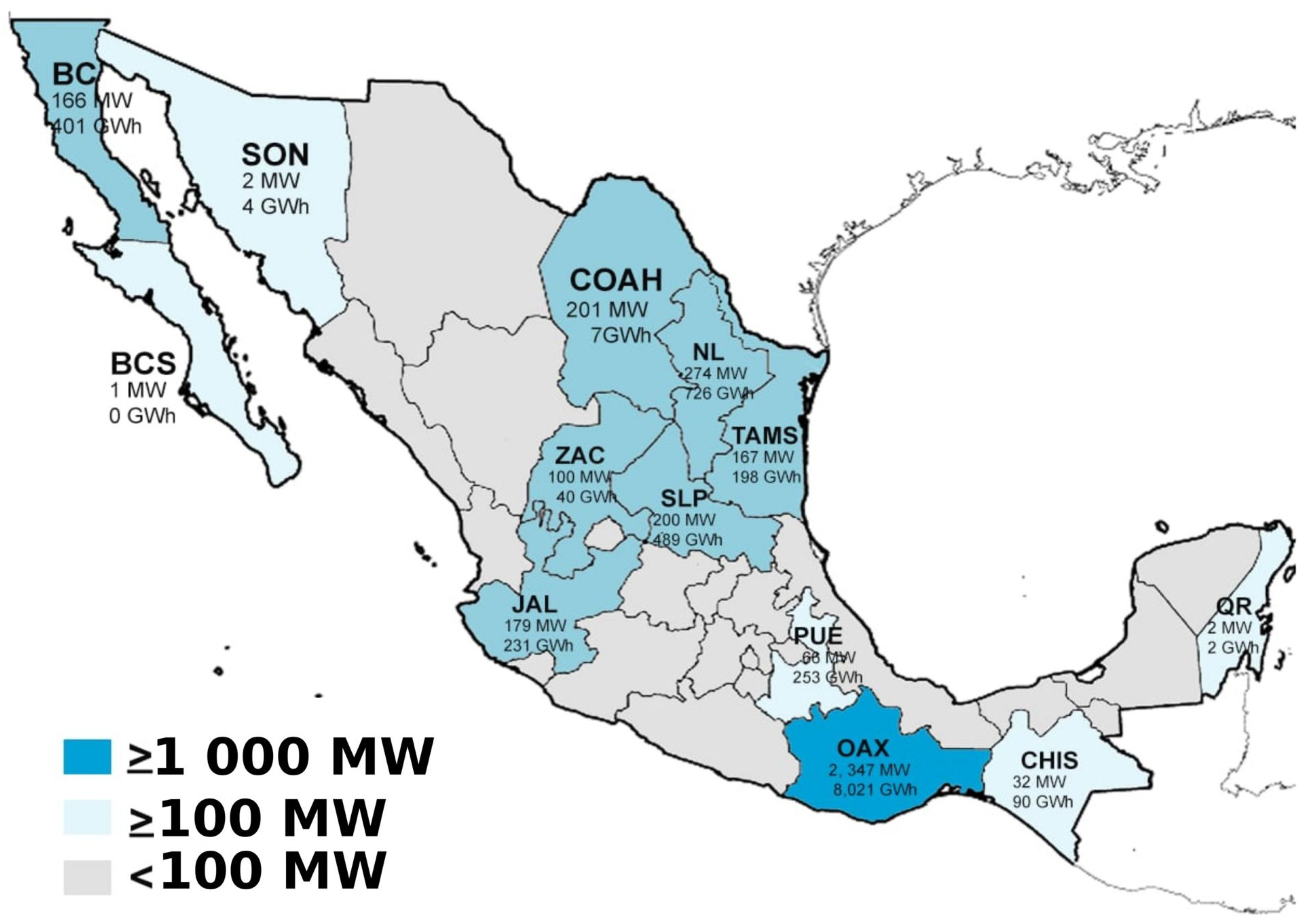
1.1. Wind Power Status Internationally and in Mexico

Producing electricity by renewable energies may reduce the continuous impact of burning fossil fuels on the environment, which contributes to global warming. Wind power has been growing rapidly around the world; the global wind power installed capacity by the end of 2017 remained above 540 GW [1].
In Mexico, the installed wind power generation capacity is close to 4 GW, with wind-generated electricity of 1976 GWh, corresponding to about 4% of the country’s generation [1]. As a consequence of the Mexican government’s target for the sector, the wind industry is aiming for an installed capacity of around 16.56 GW [2] by 2031. Figure 1 shows how the installed capacity and wind-generated electricity for 2016 are distributed in the country. The map shows 46 wind farms installed in the states of Baja California, Zacatecas, Chiapas, Jalisco, Nuevo León, Oaxaca, San Luis Potosi, Tamaulipas and Puebla [1]. The state of Oaxaca, particularly the Isthmus of Tehuantepec region, has around 63% of the total installed capacity of the country [2]. This region has a wind potential greater than 40 GW, considering only the highest wind potential areas; the wind potential is about 6 GW [3].
Mexico’s installed capacity corresponds to wind power plants; however, there are other alternatives for distributed generation using wind power. Small Wind Turbine (SWT) projects are not documented despite presenting an important wind potential [2]. This situation shows the importance of redoubling efforts to encourage wind technology as an attractive option for investors and the end-user.
This study was carried out in the Isthmus of Tehuantepec, one of the sites with the highest wind power technology implementation in the country. Experimental measurements were conducted to characterize the wind flow, determining turbulence intensity values and other statistical parameters. This information will contribute to determining sources of structural failure associated with the turbulence intensity.

1.2. Small Wind Turbine Design: Normal Turbulence Model and Turbulence Intensity

The power output depends on the atmospheric stability, which affects the profiles of mean wind speed, wind direction and turbulence across the actuator disc [4,5]. It has been demonstrated that the power output may be overestimated by about 10% without considering the turbulence effect [6,7]. Otherwise, wind turbulence contributes considerably to fatigue of the main elements of the wind turbine [8,9,10,11].
Turbulence is a micro-scale phenomenon, intrinsic to the atmospheric boundary layer that mainly depends on both the atmospheric stability and surface roughness parameters. Wind turbine and incoming wind flow interaction generate a wake in the downwind direction. At the same time, the wake interacts with the atmospheric boundary layer, resulting in a mixing region and a horizontal wake expansion caused by a turbulence transport of momentum. In wind farms, the contribution and interaction of wind turbine wake lead to the increase of the turbulence of the entire wind farm. Wake study is essential to predict the power output, fatigue and life cycle of wind turbines installed downwind of the turbine [12]. Surface roughness is the main factor increasing the fatigue loads to a wind turbine [13], and the stability of the Atmospheric Boundary Layer (ABL) has a minor influence [14]. These loads are sensitive to the structure of the ABL [15], and its effects may change in urban or forested environments [16].
Wind speed profiles are dependent on the atmospheric stability; however, the standard IEC assumes that the atmosphere is neutral stable, and the wind shear exponent is equal to 1 / 7 [17,18]. This profile is used to calculate the wind turbine rotor loads. Some studies have been carried out to assess the impact of the atmospheric stability on resource assessment of wind turbine performance and fatigue loads [9]. The impact of atmospheric stability on the extrapolation of wind speed can be studied based on observation data. This can be done by means of classifying the atmospheric stability and then extrapolating this information accordingly.
Turbulence intensity is one of the main sources of structural damage to wind turbines, and it also has an active role on the forces and bending moments acting on their structure [19], so turbulence intensity must be considered in the wind turbine design. However, meaningful time and space scales represent major challenges; the long and short term are relevant for the operation and economics of wind farms [20]. Although not all the turbulence scales affect the power output [21] or wind turbine structure [22], turbulence spectral characteristics are an important aspect to study wind characteristics for this specific location to determine possible sources o failure. It was also reported that turbulence modulates the behavior of the wind turbine performance [23]. Therefore, understanding and quantifying the turbine response to the different atmospheric turbulence scales are critical prerequisites to improve wind turbines design [24].
The main objective of this work is to characterize the wind turbulence intensity at La Ventosa, in the Tehuantepec Isthmus region of Oaxaca, Mexico, and compare it with the IEC61400 standard Normal Turbulence Model (NTM) [17,18]. Then, the reliability of the standard in the region will be studied, and the results may provide useful information to identify possible fatigue effects that compromise wind turbine structural integrity.
For wind turbine design, the IEC61400 standard has different classes based on wind speed and turbulence parameters to describe different environmental conditions. For normal wind conditions, the standard considers the wind speed distribution, the Normal Wind Profile model (NWP) and the NTM. Only the latter will be discussed in the present work. For the NTM, the representative value of the standard deviation, σ 1 , of the horizontal wind speed is given by the 95th percentile of the 10-minute average wind speed at the hub height, U h u b , and the reference value of the turbulence intensity, I r e f [17,18].
Small Horizontal Axis Wind Turbines (SHAWTs) are designed to cope with short-term fluctuations of the wind speed, turbulence and gusts, which produce unsteady loads. The international standard IEC61400-2 provides the necessary minimum requirements for loading analysis, as the NTM [17]. For the IEC61400-2, there are classes with different wind speeds, but the turbulence parameter is considered constant for all of them. However, it has been demonstrated in the literature that the NTM model roughly corresponds to the estimated conservative design turbulence intensity at wind speeds lower than 15 m/s, while it seems to be more conservative for wind speeds greater than 15 m/s except at complex sites [25]. The most pressing challenge when installing wind turbines in urban environments is to reduce the emission of noise and the vibrations generated during its operation, since in an urban environment, it is subject to strong variable loads that have the risk of damage and breakage of the device [26].
Moreover, the intensity of turbulence presented in the classes of the NTM model is not valid for complex environments, urban and forest areas and must be modified to estimate the values of turbulence intensity correctly and consequently the aerodynamic loads that affect the turbines in this type of site [16].
The design guidelines of large Horizontal Axis Wind Turbines (LHAWTs) are presented in the standard IEC61400-1, the structural design methodology of which displays the NTM. The standard takes into account a variety of environmental conditions providing classes with different wind speeds and turbulence intensity values [18]. There are some reports in which the IEC NTM model does not represent the measured data and a new turbulence intensity model is proposed [6]. Moreover, fatigue loads can be significantly larger than those prescribed by the IEC61400-1 standard, for which the daily cycle of atmospheric stability is neglected, where the highest fatigue loads occur under strong unstable convective regimes [27].
La Ventosa is an open terrain environment with a high level of turbulence, gusts and a bimodal wind speed distribution [28]. The effects of this distribution are shown in Berny-Brandt et al. [29], in which they combined structural demand hazard analysis with fatigue damage assessment applied to steel towers of wind turbines in Oaxaca, Mexico. It was found that a bimodal behavior produces a much faster fatigue damage rate than a unimodal Weibull distribution.
The objective of this work is to characterize the wind turbulence intensity by using high-resolution anemometer measurements at two heights in La Ventosa, in the Isthmus of Tehuantepec region, located in Oaxaca, Mexico. Despite the prominent development of the wind power sector in Mexico, there is a lack of available information to carry out an analysis of turbulence intensity. Furthermore, in wind energy applications, Class A cup anemometers are normally used, which do not adequately represent wind turbulence. However, due to high investment costs, high resolution, precision and 3D wind speed equipment is often lacking. In this work, two ultrasonic anemometers and a Light Detection and Ranging (LIDAR) technology were used to measure wind parameters at different heights. Wind speeds were measured at high resolution and compared with the normal turbulence intensity defined in the IEC61400 standard for the design of fatigue loads on wind turbines. The analysis was carried out for a height of 75 m to match with the common hub height. The results of the extrapolation were contrasted using the data measured by the LIDAR.
This study presents a methodology to extrapolate wind speed at a height of 75 m using two ultrasonic anemometers and a LIDAR. The method consists of classifying the wind shear exponent in terms of the ABL stability and then calculating a wind shear average value to use in the power law extrapolation. Additionally, to calculate longitudinal turbulence intensity, it was assumed that the wind direction at 75 m is equal to that of an anemometer installed at a height of 40 m. The results are compared against LIDAR measurements data, installed roughly at 180 m from the anemometer mast. Additionally, in order to study whether it is possible to conduct a structural wind turbine design using extrapolated data, the NTM model was calculated for large wind turbines using both extrapolated and LIDAR data, and the results were compared.
This paper is organized as follows: First, the theoretical elements related to turbulence intensity calculations are presented. Then, the methodology, which comprises site measurements and data processing, is presented. Then, the results and discussion regarding power law extrapolation are presented, as well as the comparison of the turbulence intensity against the NTM model. Finally, the main conclusions of this research are presented.

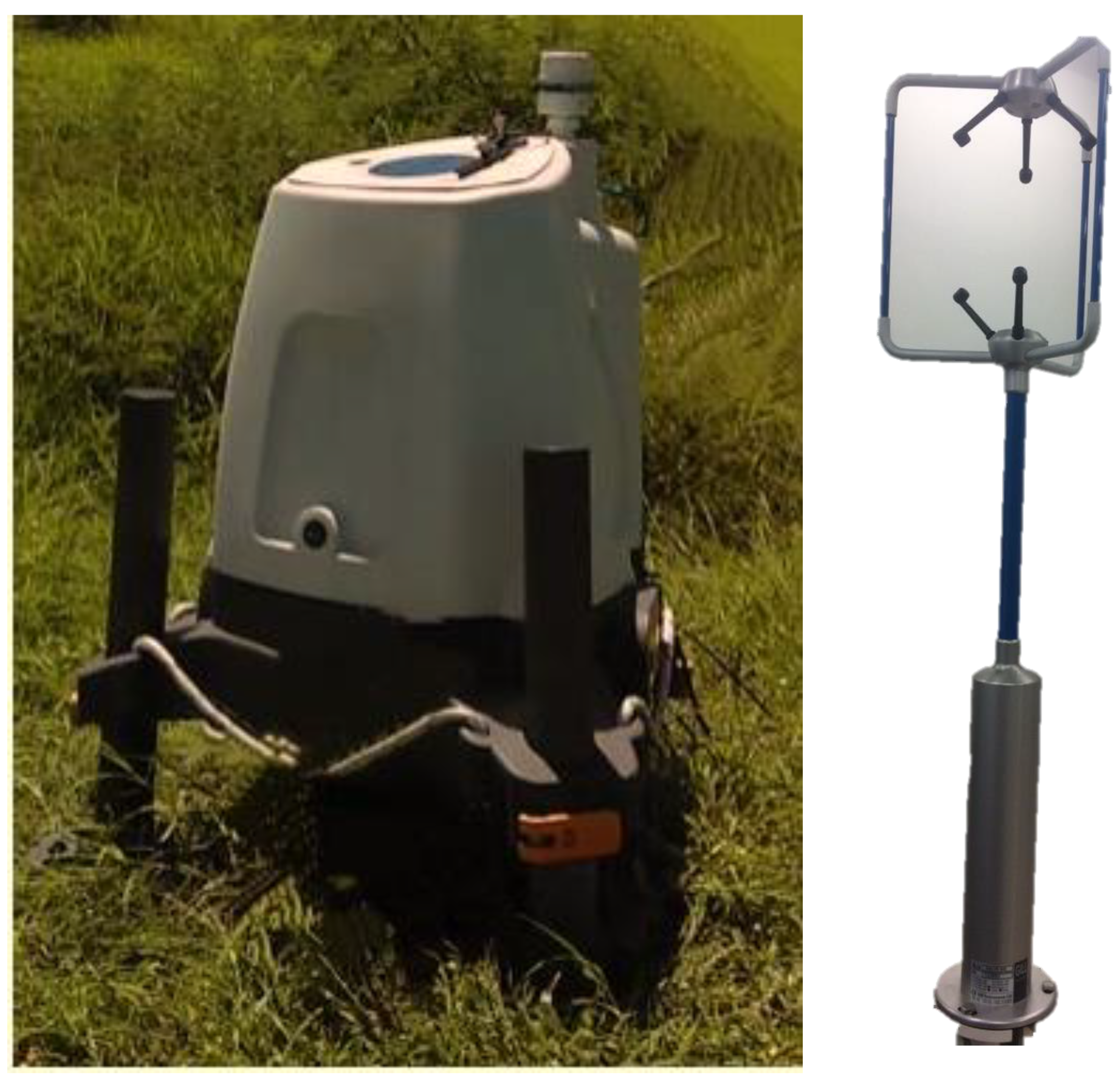
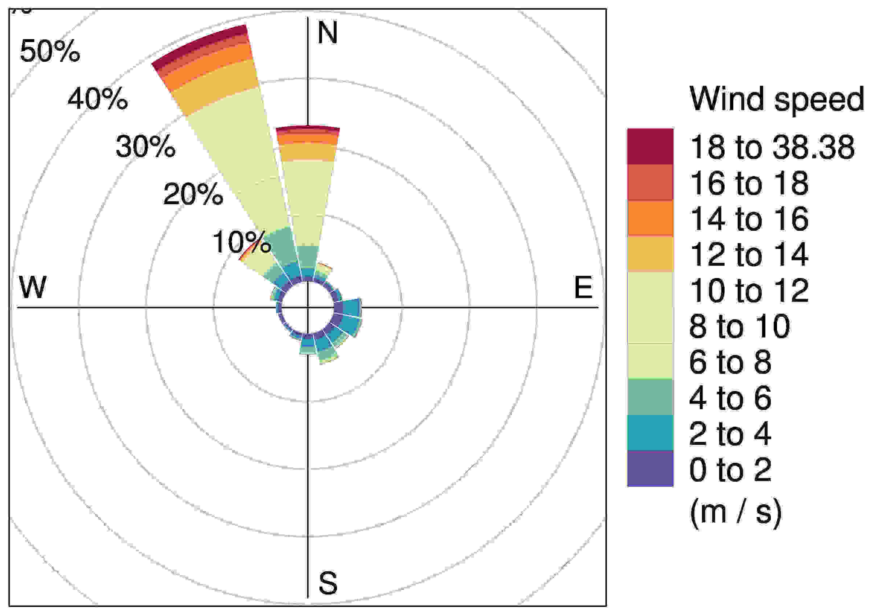
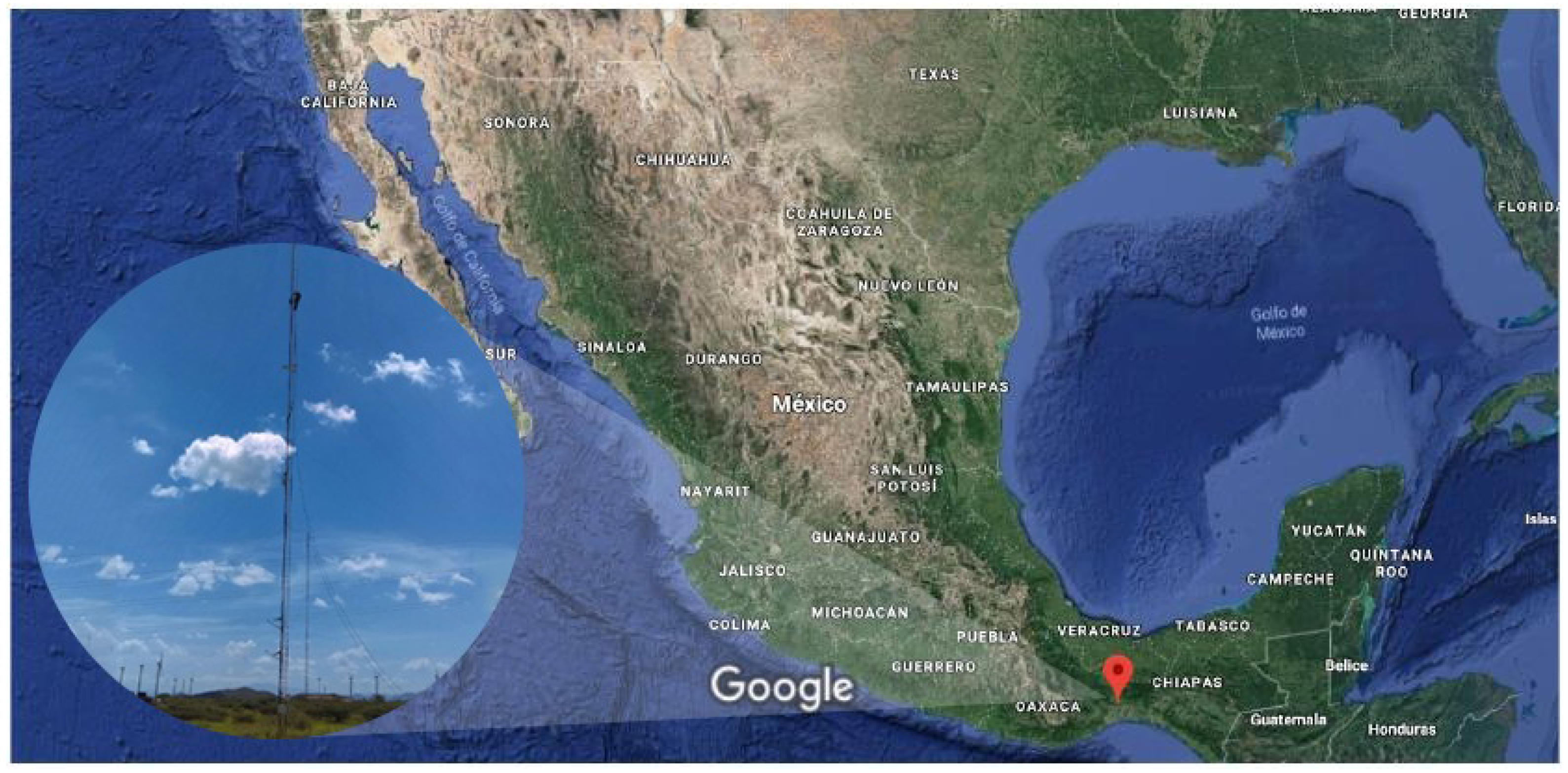
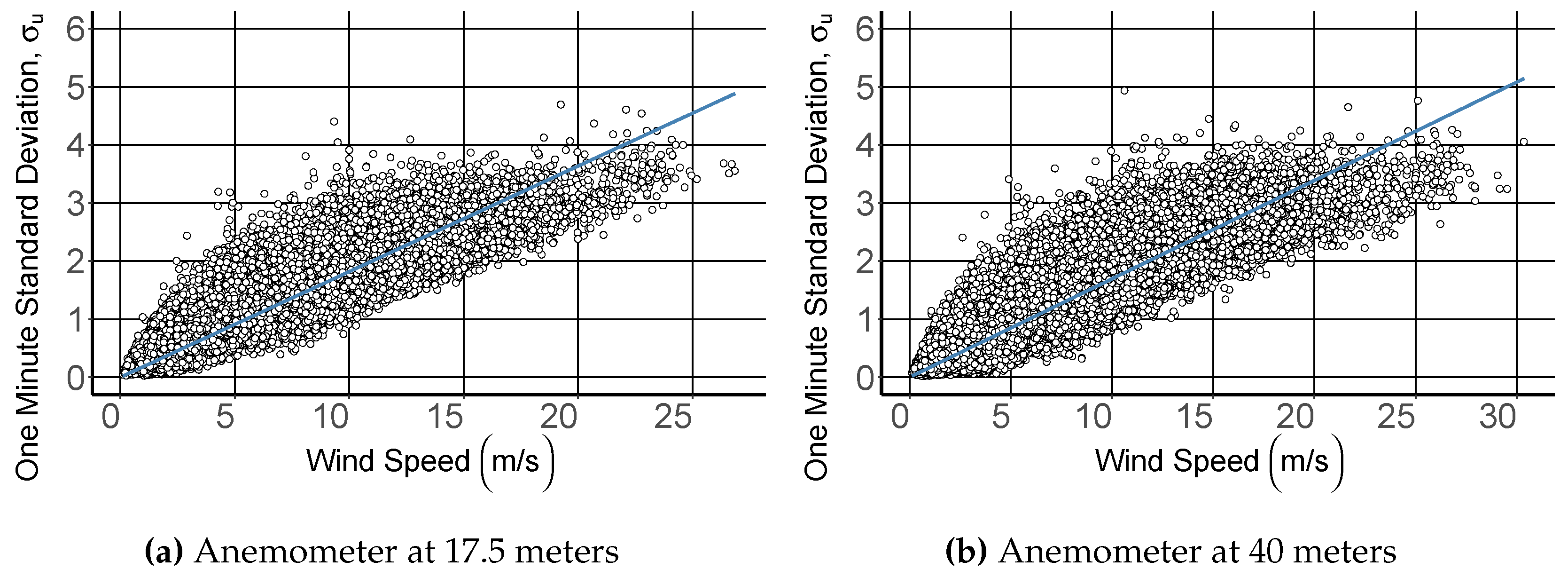
2. Site Measurements and Data Processing

Measurement campaigns were conducted at La Ventosa, in the Tehuantepec Isthmus region of Oaxaca, Mexico (coordinates: 16 ° 32 40.8 N 94 ° 57 09.0 W). In Figure 2, the location of La Ventosa is marked, and the 40-m high lattice mast is shown where two 3D Gill WindMaster ultrasonic anemometers were installed (see Figure 3). The Isthmus is of special interest because it is situated near an unusually warm ocean current, which, combined with the area’s temperature and pressure gradient, results in a strong northern wind, which translates into a high level turbulence and gust.
Measurements were obtained at two elevations using a precision 3D anemometer Gill WindMaster: 17.5 and 40 m above the ground level. Both anemometers offer outputs at 20 Hz (32 Hz optional) of temperature, pressure and the three components of wind speed. Data were measured and recorded at a frequency of 1 Hz to characterize wind turbulence, from September 2017 to July 2018.
The power law model is one of the most used tools for extrapolating wind speed in the vertical direction. In the present work, the extrapolated wind speed consists of classifying the wind shear exponent in terms of the ABL stability and then calculating a wind shear average value to use in the power law extrapolation. Van de Berg [30] concluded that wind speed is higher in a stable atmosphere (during the night), and if a neutral wind shear exponent is used in the power law model to extrapolate the average wind speed, the average wind speed and the wind turbine noise levels can be underestimated.
To validate the extrapolated power law methodology, a comparison between the extrapolated mean wind speed and measured data provided by the ZephIR LIDAR 300 (see Figure 3) was carried out. LIDAR technology provides remote wind measurements along 10 different simultaneous heights defined by the user in a range between 10 and 300 m. The LIDAR measures 50 points every second within a 360 ° scanning range, providing a high sampling rate in complex and fluctuating air flows. Furthermore, the turbulence intensity calculated through measurements taken by the LIDAR, as well as extrapolated by the power law is also analyzed.
A summary of the sampled data is presented in Table 1, where the wind speed statistics of the anemometers, the LIDAR and the data extrapolated are shown. The maximum value of wind speed corresponds to the equipment, LIDAR, which conducts measurements at a greater height; it is about 40 m/s with an approximate mean value of 9 m/s.
Also presented are the extrapolated data at 75 m, where the maximum value is close to 61 m/s with a mean of 9.70 m/s. The measured wind direction is consistent with the phenomenology of the site, which is represented in Figure 4, where the dominant winds are in the north and north-northwest (N-NNW) direction.
Data recorded by using the two ultrasonic anemometers and the LIDAR 300 are analyzed to investigate the effects of turbulence intensity in the structure of wind turbines in La Ventosa. Ultrasonic anemometers data were recorded at a frequency of 1 Hz from September 2017 to July 2018. LIDAR data were sampled at a frequency of 50 Hz and recorded at 0.06 Hz from September 2017 to July 2018. Working with large amounts of data involves carefully reviewing time series using incomplete or unreliable information. Once we had both anemometer and LIDAR data series of 324 days with no errors or missing data, the data were filtered to produce datasets using 10-min mean time, in accordance with the standard IEC61400-2 [17] for the small wind turbine design and the standard IEC61400-1 [18] for the large wind turbine design.
For each mean time dataset, the behavior of turbulence intensity was analyzed at different heights, and the longitudinal turbulence was calculated and compared with the standard reference values. Moreover, the reference turbulence intensity, I 15 , was calculated through a linear fit using Equation (3) of the scatter standard deviation versus the mean wind speed [31]. These results are compared with the reference turbulence intensity values reported in the NTM of IEC61400-2.

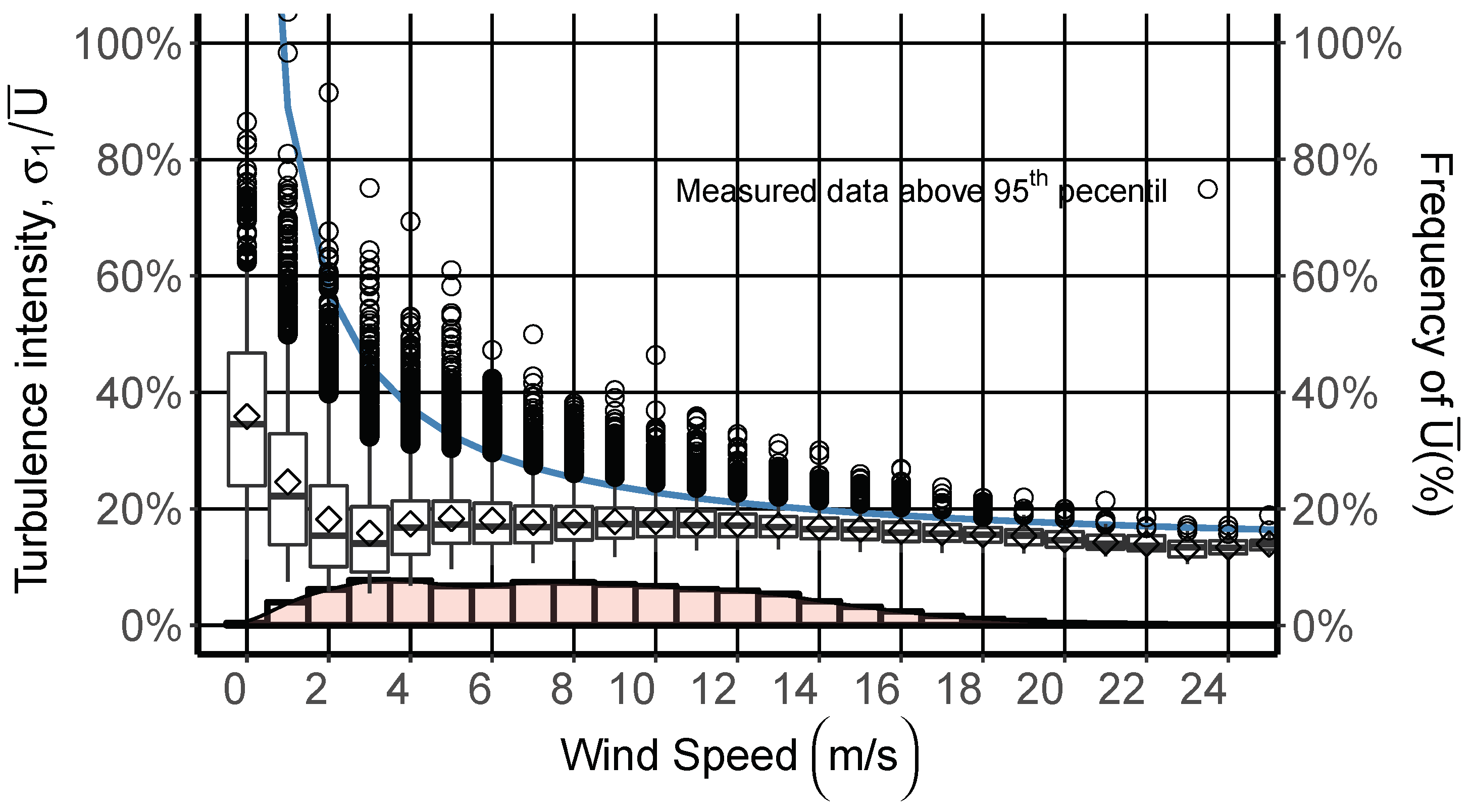
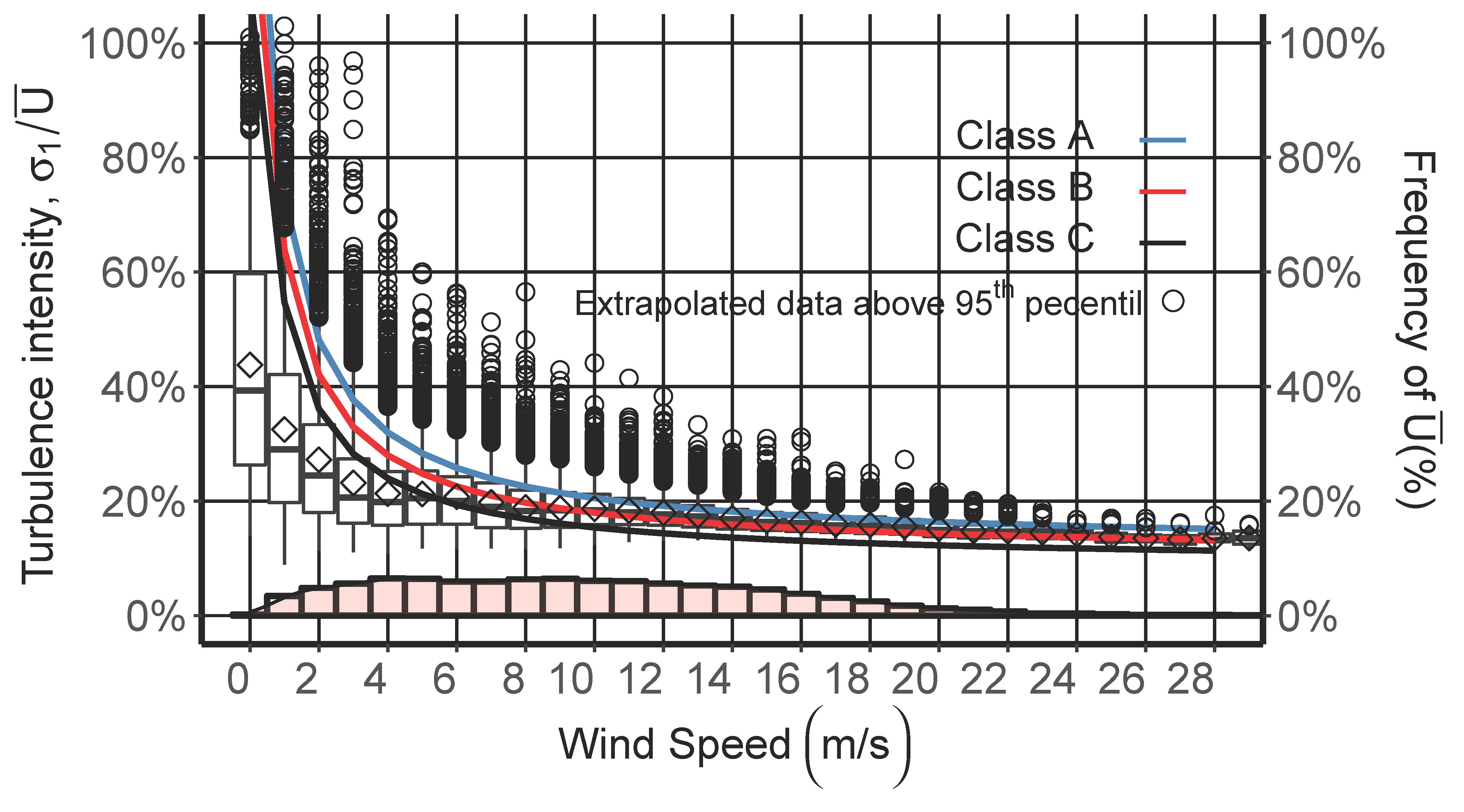
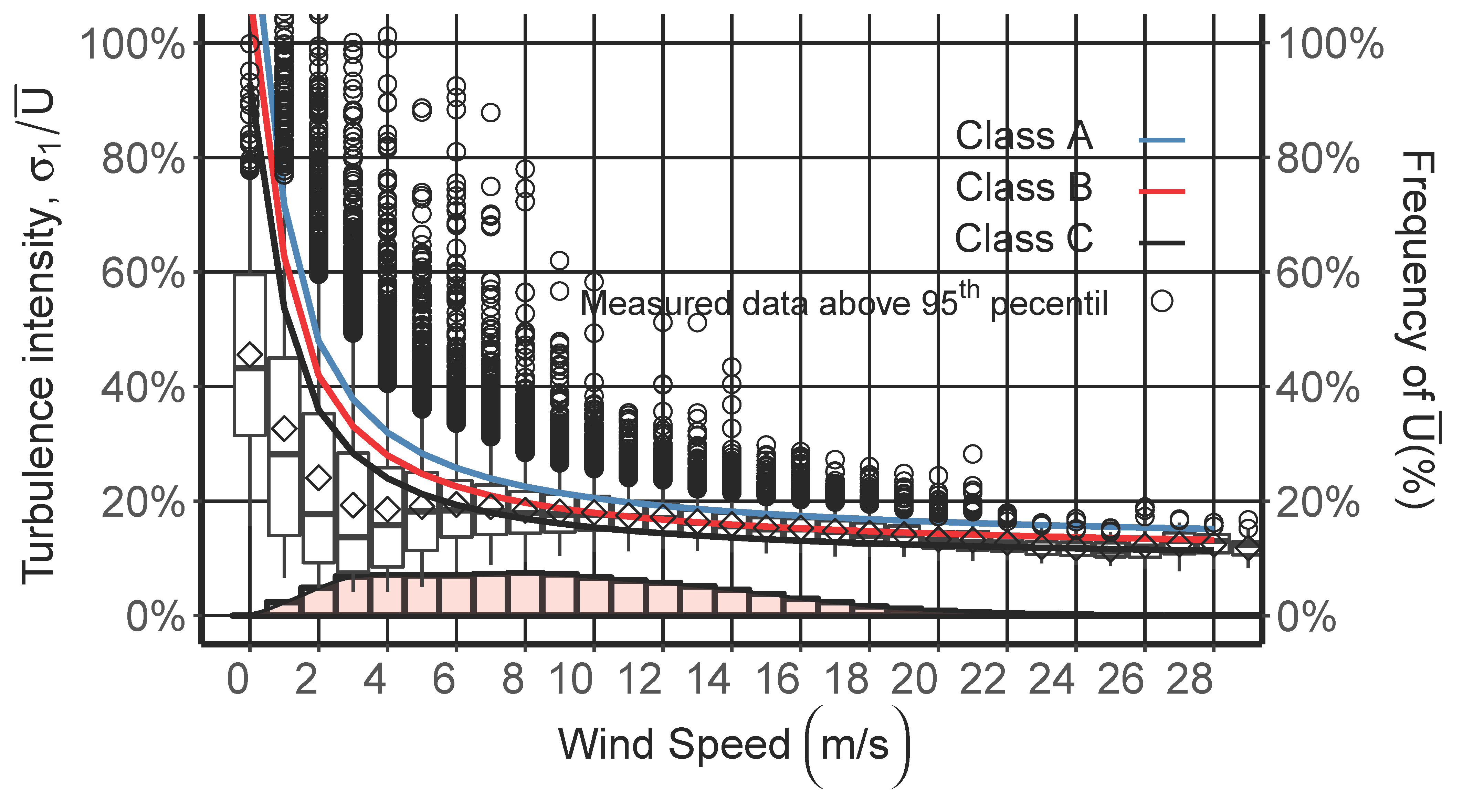
3. Turbulence Intensity

In wind power, turbulence is a transport process that is intrinsic to the atmospheric boundary layer that affects the power performance of a wind turbine. Wind fluctuations induce unsteady loads on wind turbine blades, which can cause fluctuations in the electric power output, as well as structural and drive-train problems. Moreover, atmospheric turbulence in the incoming flow induces unsteadiness around the surface that leads to the propagation of sound [32].
The average power available in terms of turbulence intensity and average wind speed is calculated by [33]:
P W = 1 2 ρ A 1 + 3 I 2 V ¯ 3
where ρ is the air density, I is the turbulence intensity and A is the rotor swept area. Equation (1) suggests an increment in the available power as a result of the inherent turbulence in wind flow.
Terrain roughness, temperature vertical gradients and orography effects are factors determining the turbulence and expected energy production levels. Turbulence is an important factor to consider when unsteady load magnitudes are determined on blades, as well as overall vibration levels on the mechanical elements of the wind turbine.
A common technique to characterize wind turbulence in a wind speed time series is to assume the phenomena as normally distributed. Wind speed time series are commonly sampled at 1 Hz and recorded at longer average times, where the corresponding standard deviation is also calculated. Therefore, turbulence intensity may be estimated as the ratio of the standard deviation and the mean for the same period of time.
I = σ U ¯
where U ¯ and σ are the average value and standard deviation of wind speed, respectively.
Fatigue loads are influenced by wind turbulence acting on the wind turbines, and they become important to model the standard deviation of fluctuating wind velocity accurately. The NTM is presented in the standard to define turbulence under normal operating conditions. The standard has different classes based on wind speed and turbulence parameters to represent different environmental conditions. These classes are defined in terms of reference wind speeds and reference turbulence intensity parameters. For each class, there are different values of reference wind speed, but the reference turbulence intensity parameter is constant, taking the value of 0.18 [17]. For the NTM, the representative value of the standard deviation, σ 1 , of the horizontal wind speed is given by the 95th percentile of the 10-min average wind speed at the hub height, U h u b , and the reference value of the turbulence intensity, I r e f [17].
σ 1 ( 95 % ) = I r e f 15 + a U h u b a + 1
where I r e f is the expected value of turbulence intensity at 15 m/s, U h u b is 10-min average wind speed and parameter a is the model parameter to estimate the mean value and the standard deviation σ 1 .
This model is adjusted to design turbines for a load analysis with turbulence levels within the range of wind speeds between 10 and 25 m/s [34].
A similar approach is followed by NTM IEC61400-1 where the turbulence intensity model may written as follows:
I 90 % = σ 1 ( 95 % ) U ¯ = I r e f a + 1.28 α + b + 1.28 β U ¯
where U ¯ is the 10-min mean wind speed, I r e f is the expected value of turbulence intensity at 15 m/s and the parameters a, b, α and β are the model parameters to estimate the mean value and the standard deviation of σ 1 . The variable values of Equation (4) are summarized in Table 2, where the difference between standard IEC for small and large wind turbine applications is the reference turbulence intensity, I r e f [18].
A common approach for turbulence analysis is to consider dividing wind velocity into two parts: the mean value and the fluctuating part. Microscale turbulence is a three-dimensional phenomenon and therefore may be described by its longitudinal, u = u ¯ + u , lateral, v = v ¯ + v , and vertical, w = w ¯ + w , components [35].
The mean wind speed value, u ¯ , as well as the v ¯ and w ¯ components can be defined by [35]:
u ¯ = 1 N i = 0 N u i
where N
is the number of elements in the wind speed dataset.
The standard deviation is defined as the square root of the variance:
σ 1 = 1 N i = 0 N u 2 1 / 2
Near the ground, the turbulence intensity might be expected to increase as the mean wind speed, U ¯ , increases. For this reason, a dimensionless measure of the turbulence intensity, I 1 , is often defined as:
I 1 = σ 1 U ¯
Similar definitions apply to the lateral and vertical velocities, v and w:
I 2 = ( v ) 2 ¯ 1 / 2 U ¯ = σ 2 U ¯
I 3 = ( w ) 2 ¯ 1 / 2 U ¯ = σ 3 U ¯

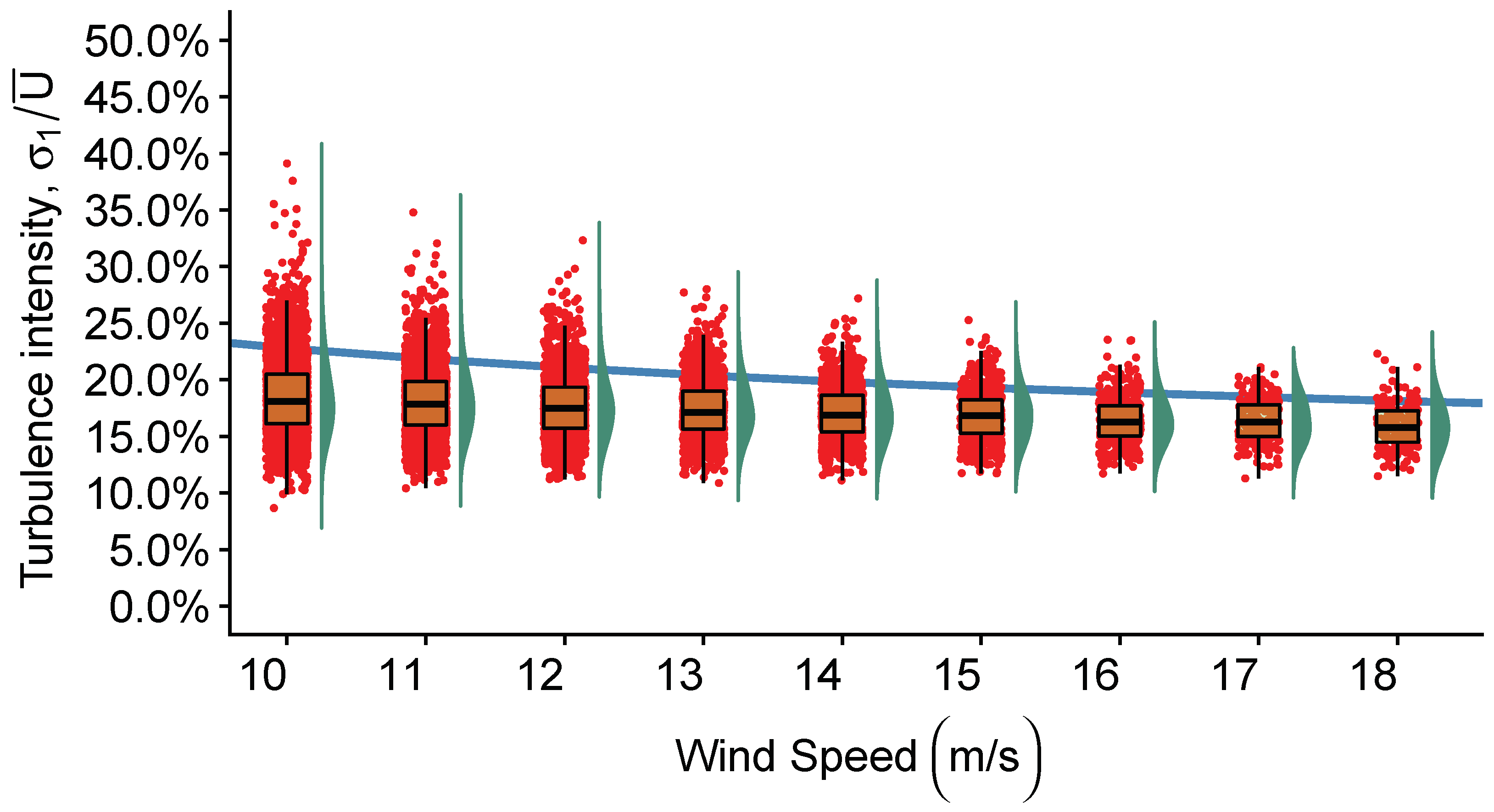
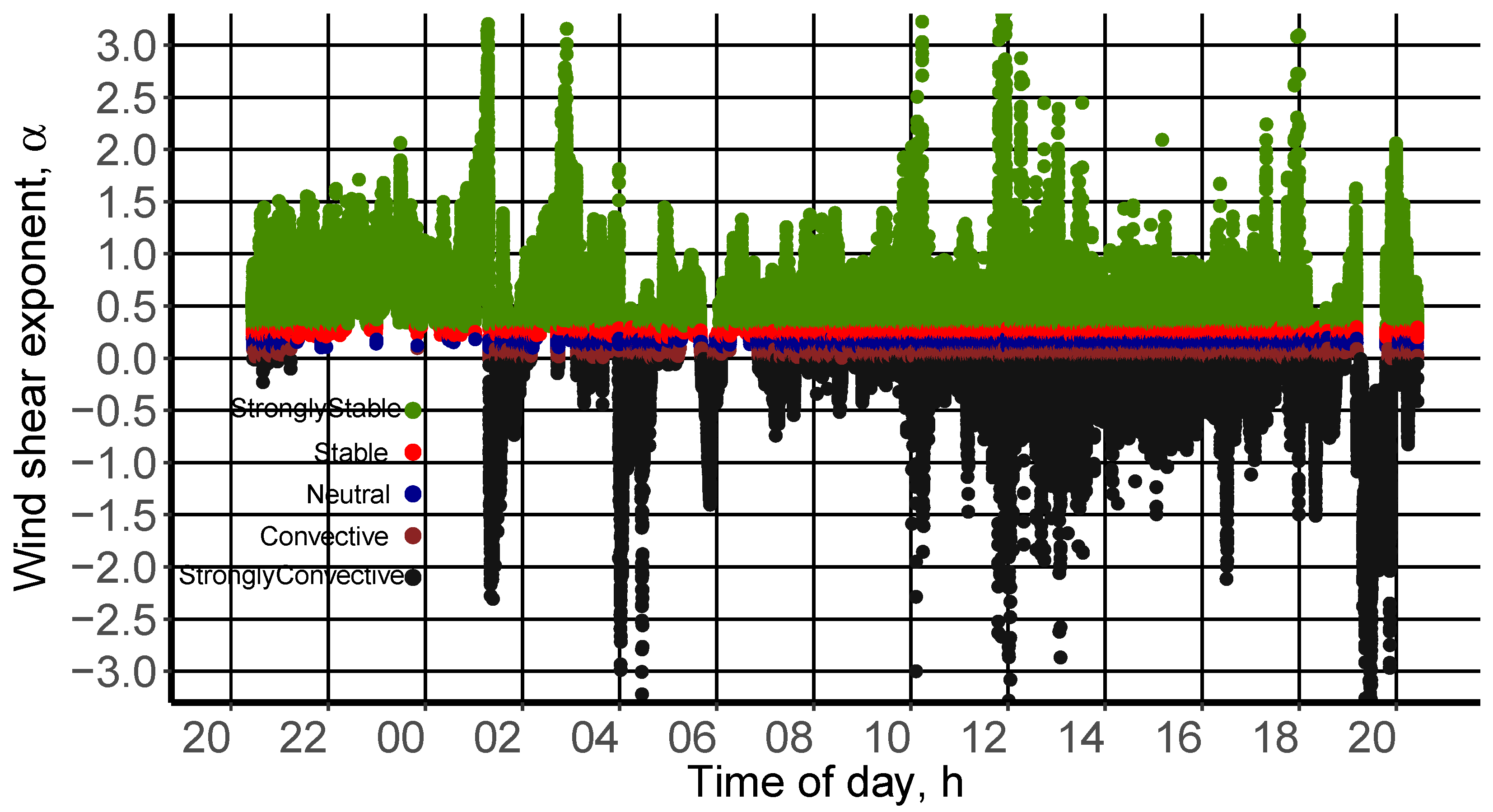
4. Results and Discussion

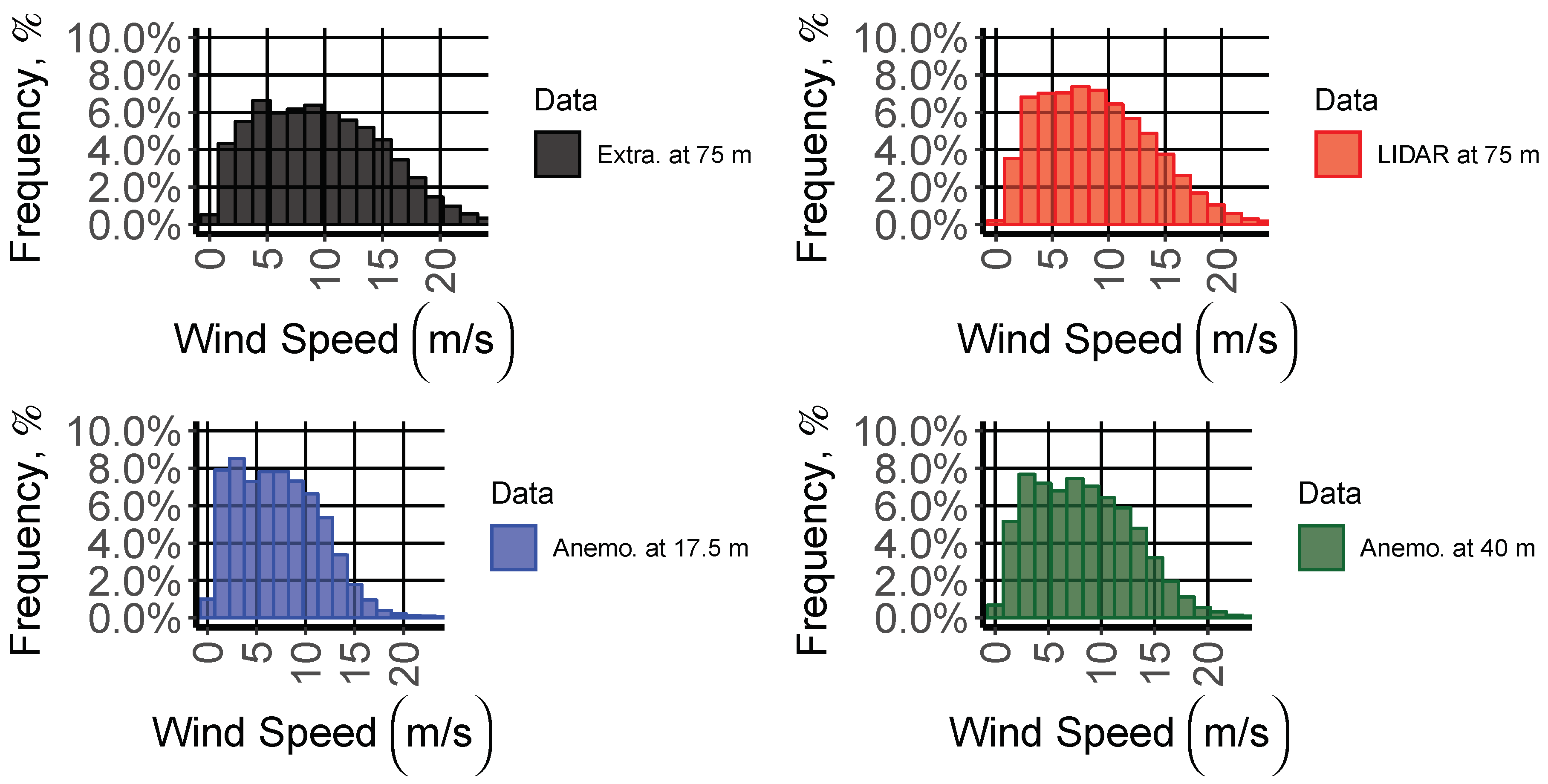
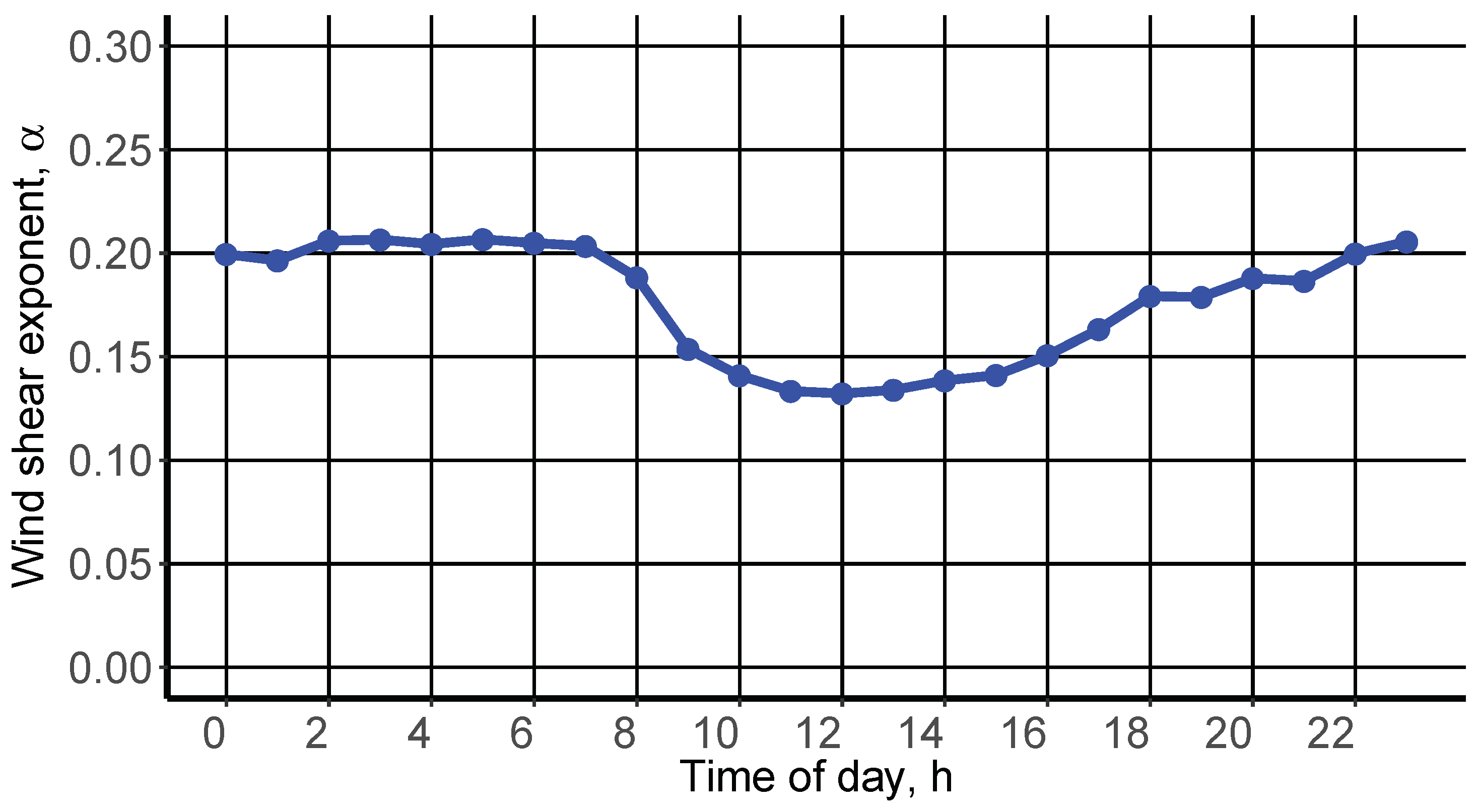
4.1. Power Law Extrapolation

Wind speed changes with the height and has a great influence on the assessment of wind energy resources and the design of wind turbines. These wind speed changes have a major impact for large wind turbine applications, where the rotor hub height is usually above 75 m. However, in the present work, the highest installed anemometer was at 40 m above ground level; for this reason, a velocity extrapolation was necessary. There are two mathematical models commonly used to quantify the vertical profile of wind speed over flat terrain. These are the logarithmic law and the power law. The former can be derived theoretically from basic principles of fluid mechanics. By contrast, the power law is empirical and commonly used in wind engineering to define vertical wind profiles because it is simple and direct. The basic equation of the wind shear power law is:
u ( z ) = u R z z R α
The stability of the atmosphere is governed by the vertical temperature distribution resulting from radiative heating or cooling of the Earth’s surface and the subsequent convective mixing of the air adjacent to the surface. Atmospheric stability states are classified as Strongly stable (Ss), Stable (S), Neutral (N), Convective (C) or Strongly convective (Sc). These classifications can be defined in terms of the wind shear exponent, as is shown in Table 3.
Because atmospheric stability is governed by solar radiation with its diurnal cycle, we can expect that wind shear will also exhibit a diurnal cycle. This is typically the case, as illustrated in Figure 5, by wind shear variation with time of day, calculated from the measured 1-Hz sampling rate data for La Ventosa, Oaxaca, Mexico, at two different heights reported in the present work: 17.5 and 40 m. During the period of measurements, the atmospheric stability was predominantly strongly stable and strongly convective, with 34.8% and 24.0%, respectively. The convective, neutral and stable stabilities were 12.6%, 14.5% and 14.1%, respectively.
Figure 5 represents the value of α changing every 1 s. Figure 6 shows the hourly variation of the binned wind shear exponent for a typical day, so it is clear that the wind shear exponent varies with time; it is also affected by the surface roughness and atmospheric stability.
During the period of measurements, the atmospheric stability was predominantly strongly stable and strongly convective, with 34.8% and 24.0%, respectively. The convective, neutral and stable stabilities were 12.6%, 14.5% and 14.1%, respectively. Furthermore, from Figure 6, it can be concluded that α is a variable quantity ranging from around 1/7 during the daytime to approximately 1/5 during the night.
Table 4 presents the wind shear exponent under different atmospheric stabilities used to calculated the wind speed at a height of 75 m using Equation (10) and a wind speed time series of 1 Hz. The values shown in Table 4 are obtained by classifying the wind shear exponent in terms of the ABL stability; then, from this stability classification, an average wind shear exponent was calculated.
Figure 7 shows the wind speed frequency distributions for the anemometric and LIDAR measured data and the 75 m high extrapolated data. The figure shows that the extrapolated data distribution was as expected, although the peak in the distribution was underestimated due to the difference in the recorded frequency of extrapolated and LIDAR time series, 1 and 0.06 Hz, respectively.

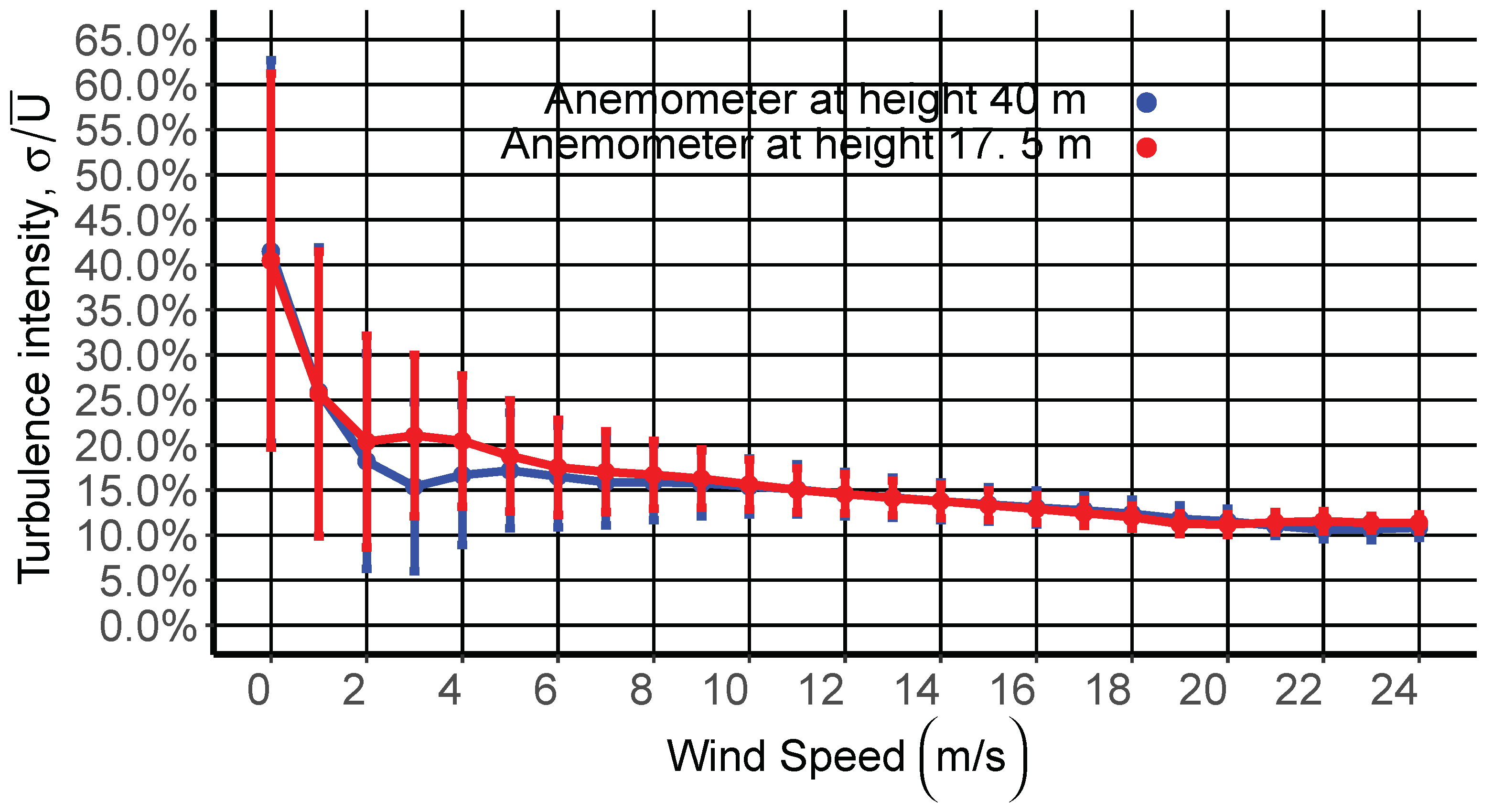
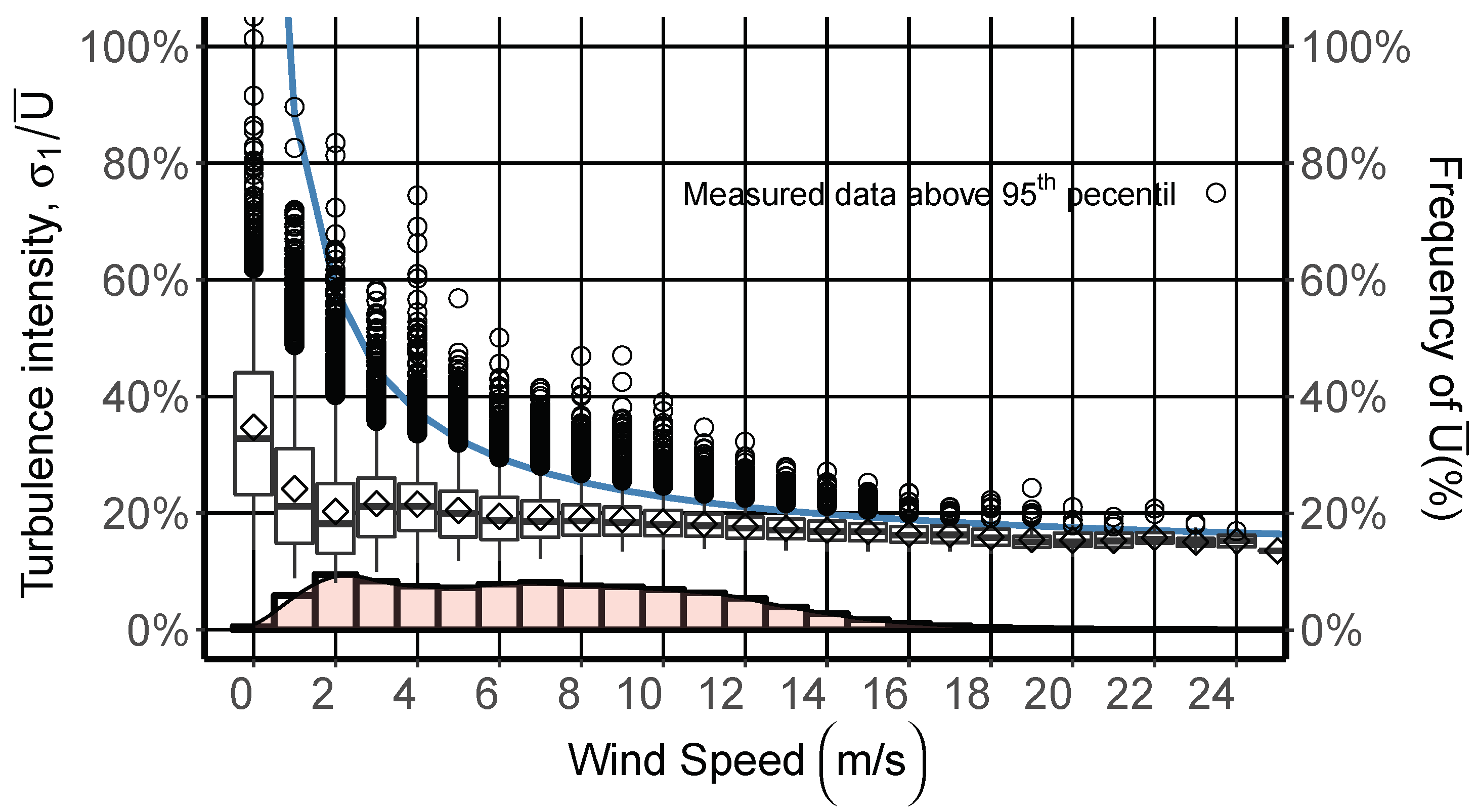
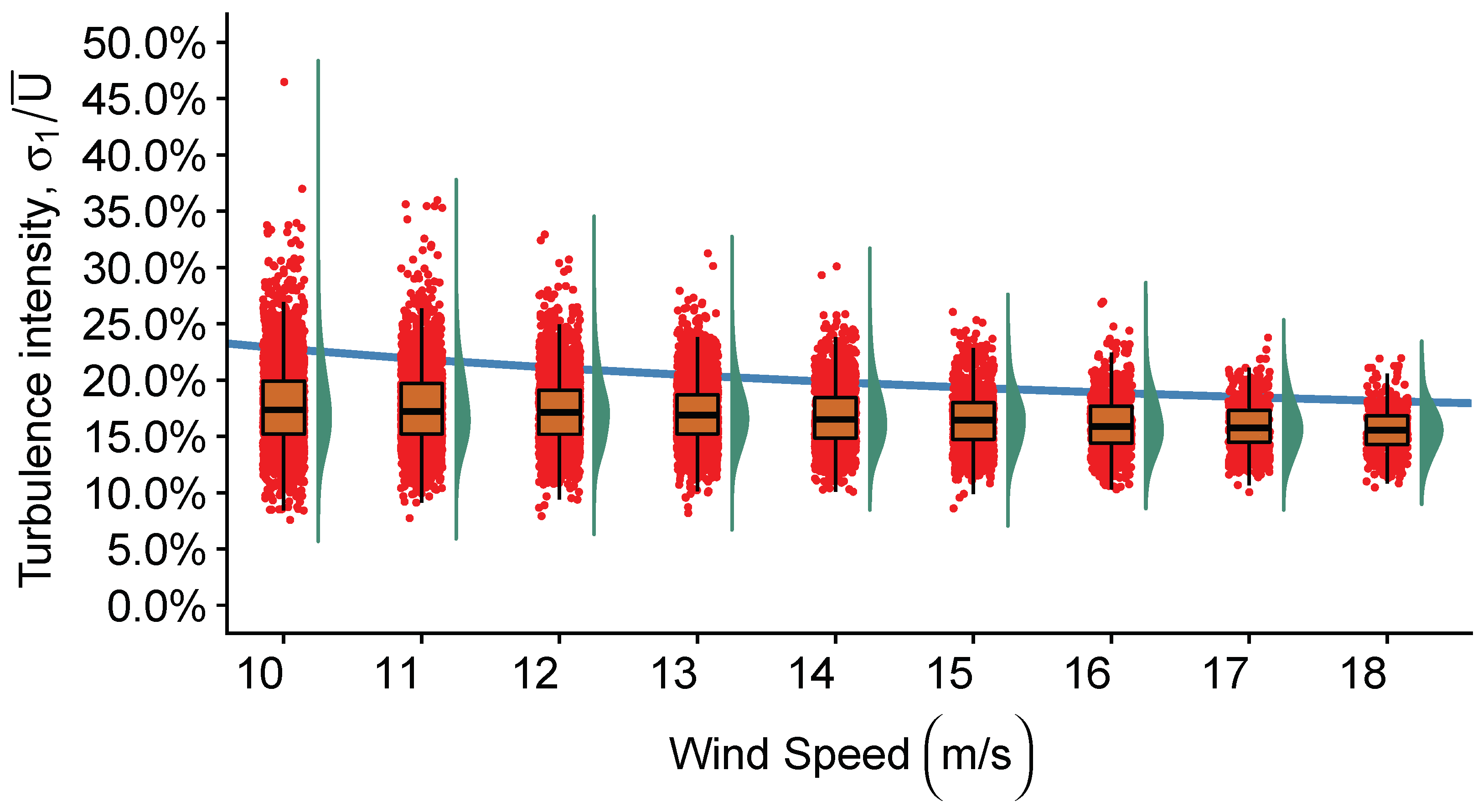
4.2. Characterization of Turbulence Intensity

The ever-present wind turbulence is the main issue driving this work, since unavoidable rapid changes in wind direction produce unstable and cyclically variable loads as soon as they strike the rotor. Figure 8 presents the total turbulence intensity, 2 / 3 k , where k is the turbulent energy; a 10-min average was used for both heights. Note that the error bars in Figure 8 represent the average ± standard deviation of binned turbulence intensity values. It is clear that the one closest to the ground presents a greater turbulence intensity for wind speeds ranging from 1 to 5 m/s; however, for higher wind speed values, it remains approximately constant. Note that the error bars represent the standard deviation of binned turbulence intensity values.
As has already been mentioned, the calculated longitudinal turbulence intensity was compared with the NTM of IEC61400-2. The results are shown in Figure 9 and Figure 10, where the standard NTM model assumed the reference value as I r e f = 0 . 18 (blue line). In both figures, a box plot is presented, which is based on the minimum and maximum within the range Q 1 , 2 ± 1 . 58 I Q R , first quartile ( Q 1 ), median, third quartile ( Q 2 ) of the measured data. In the box plot, the central rectangle spans the first quartile to the third quartile (IQR). A segment inside the rectangle shows the median, and the lines above and below the box show the locations of the minimum and maximum. Data were also displayed above the 95th percentile of the measured data, in order to present the data that were not considered in the box plot, but have to be taken into consideration for studying fatigue sources. The diamond shape located inside the box shows the average turbulence intensity value. The wind speed frequency distribution is also presented. It was found that almost all of the 95th percentile values were above the normal turbulence model, which roughly corresponds to 388 h of exposure of values out of the reference turbulence intensity design, which may contribute to fatigue loads on a wind turbine.
In this research, it has been noted that turbulence intensity varies with height and was also higher than low heights since the roughness and shear effects have a greater impact on the behavior of the flow. In general, there was a wide range of wind speed in which the notches had values above the reference intensity, I r e f (0.18), intersecting the NTM model.
Figure 11 and Figure 12 show, for a range of wind speeds from 10 to 18 m/s, the raw data measured (red dots), the probability distribution, the box graph and the NTM model (blue line). It can be seen clearly that the NTM model was superimposed on the box plot notches, and it is possible to visualize the data that were beyond the limit Q 2 + 1 . 58 I Q R . Despite the fact that the average turbulence intensity at the reference wind speed (15 m/s) was below the I r e f , the NTM model should be reconsidered for the present case study.
Hence, this is something to be considered when designing a wind turbine since most turbines are built in accordance with the standard, and they are not designed to allow turbulence intensity above 0.18. Therefore, it may be concluded that it is not recommended to generalize the reference turbulence intensity values for the entire wind speed range, because wind speed fluctuations that cannot be captured by the model can have a negative effect on the fatigue cycle of the wind turbine.
Figure 13 shows a linear fit of the scatter standard deviation against wind speed for both heights: 17.5 and 40 m for the 10-min mean time. These calculations were conducted using Equation (3) by means of least squares of the data standard deviation [37]. Table 5 presents the calculated values of characteristic turbulence intensity, I 15 , for the different heights; it can also be seen that the calculated reference turbulence intensity decreases as height becomes greater. Moreover, this parameter is sensitive to the averaging period, increasing as the averaging period does. This increase is due to the use of longer averaging periods that have a higher probability of capturing a wider range of wind conditions and hence a greater standard deviation of wind speed.
The calculated turbulence intensity values from the two anemometers and LIDAR technology are compared with the values proposed by standards IEC61400-1 and IEC61400-2, respectively. It can be seen that the calculated turbulence intensity reference values were quite close, but this was considering a reference wind speed value of 15 m/s. However, it is recommended to not generalize for all wind speed values, since at lower wind speeds, turbulence intensity can reach higher values, which implies a higher scattered standard deviation, and the wind turbine blade may suffer a structural failure.
The aforementioned study on turbulence intensity may have a great impact on small wind turbine fatigue load design, and it may be possible that small wind turbines endure extreme meteorological conditions. However, there is no guarantee that a wind turbine blade will not reach the breaking point due to other factors, i.e., electrical generator and drive-train failures, among others (and become a problem for human health and safety). The above adds a high degree of complexity to the aerodynamic and structural design of wind turbines for this region.
Due to high inversion costs, there is a scarcity of data measured at a height of 75 m or even higher for decision-making related to techno-economic analysis or wind turbine design. Therefore, in this work, a methodology was described to extrapolate wind speed at a height of 75 m using two ultrasonic anemometer-measured datasets using a power law model. The method consists of classifying the wind shear exponent in terms of the ABL stability and then calculating a wind shear average value to use in the power law extrapolation. A turbulence intensity analysis was performed for the 75 m high extrapolated data; the analysis is also presented using measured data obtained by a ZephIR LIDAR 300 for a height of 75 m. The latter is to compare the turbulence values and find out whether it is possible to use extrapolated data to design wind turbines. Figure 14 and Figure 15 show the NTM IEC61400-1 standard for the three classes (A, B and C), where each class used different values of reference turbulence intensity as reported in [18]. The binned turbulence is also shown for the 75 m high data and the 75-m ZephIR LIDAR 300 grouped together with the NTM model. Both figures agree that the classes reported in the IEC61400-1 are not adequate for designing large wind turbines because most of the fluctuation of the wind flow is above the class design model within velocities ranging from 6 to 21 m/s, which coincide with the fully-operational wind turbine, which may lead to undesirable fatigue loads and serious structural damage. In conclusion, the measured data did not fit with Classes A, B and C and would have to be designed as Class “S”.
The LIDAR measured data were compared against the extrapolated data using the power law model. Despite the predicted turbulence intensity being high for lower velocities, the overall behavior is reasonably well predicted.
As can be seen in this study, extremely turbulent conditions were observed, with rapid changes in wind speed, known as gusts. This exposes the structure to stress and impairs performance, because it produces resonance in the turbine and in the support structure. In addition, these changes are not uniform in the area of the rotor, which leads to all the blades being unable to compensate equally, resulting in less energy generated. On the other hand, these gusts imply that the wind turbine would have to be designed with more rigidity and strength to withstand these induced vibrations, which would increase the material and production costs. However, the design analysis will have to go deeper to identify the correct maximum loads and load spectrum, using data measured in the field.

5. Conclusions

This work presented a characterization of turbulence intensity for small and large wind turbine applications for an open terrain located at La Ventosa, Oaxaca, Mexico, by means of data measured using two ultrasonic anemometers installed at two different heights and LIDAR technology.
As a first step in the analysis, wind speed time series from the ultrasonic anemometers were extrapolated and compared with data measured by the LIDAR at 75 m. The extrapolation of the wind speed was carried out at 75 m by classifying the atmospheric stability using the wind shear exponent. It was observed that the atmosphere is strongly convective and stable most of the time during the measurement period. Overall, the prediction data were in accordance with the data measured with the LIDAR, despite the predicted turbulence intensity being high for lower velocities.
Next, the turbulence intensity was calculated following the methodology established in the international standard for the design of large and small wind turbines. It could be observed that for a range of wind speeds from 2 to 24 m/s, some of the measured values of the turbulence intensity were greater than that those recommended by the standard. These values correspond to 388 hours of fatigue loads not considered for wind turbine design. This may lead to unreliable designs, which may suffer structural damage. Therefore, the region should be considered as Class “S”.
Finally, this study focused on characterizing the turbulence intensity in a site—despite extreme meteorological conditions with rapid changes in wind speed—and analyzing the viability of the design of small- and large-scale wind turbines using the NTM presented in the IEC61400. It was determined that the classes presented in the international standards IEC61400 could be unsuitable for the site, resulting in an important structural failure, as well as a decrease in energy production.
The results presented in this contribution are useful for the detection of a possible source of failure associated with the fatigue loads of wind turbines installed in the region. Furthermore, the developed turbulence intensity analysis may be used to design reliable technologies for small wind turbine applications in the region. These are factors that will contribute to the development of the wind power sector in Mexico.

Author Contributions

Conceptualization, C.A.L.-V., O.R.-H. and R.C.-A.; Data curation, C.A.L.-V.; Formal analysis, C.A.L.-V., O.R.-H. and R.C.-A.; Funding acquisition, O.R.-H. and R.C.-A.; Investigation, C.A.L.-V., R.C.-A., O.R.-H., G.H.C. and J.L.M.; Methodology, C.A.L.-V., O.R.-H. and R.C.-A.; Resources, O.R.-H., R.C.-A. and G.H.C.; Software, C.A.L.-V.; Supervision, R.C.-A. and O.R.-H.; Validation, C.A.L.-V.; Visualization, C.A.L.-V.; Writing—original draft, C.A.L.-V.; Writing—review & editing, O.R.-H., R.C.-A. and O.A.J.

Funding

This research was funded by Dirección General Asuntos del Personal Académico, Universidad Nacional Autónoma de México (DGAPA, UNAM) (PAPIIT-IA107416); CONACYT-SENER-Sustentabilidad Energética 272063.

Acknowledgments

C. A. Lopez-Villalobos would like to thank the Science and Technology Council of Mexico (CONACYT) for my PhD scholarship. C. A. Lopez-Villaloboswould also like to thank Maximiliano Valdez for both technical support and valuable recommendations. We would like to thank the project IA107416, “Aeroacoustic study in horizontal axis wind turbines”, call Program of support for Research and Technological Innovation Projects(PAPIIT-UNAM), for supporting the development of this research work. We would like to thank the project 272063, “Strengthening of the field of Wind Energy in the Doctoral Program in Engineering Field of Knowledge in Energy based in the Institute of Renewable Energies of the National Autonomous University of Mexico”, call Institutional Strengthening for Energy Sustainability and fund CONACYT-SENER-Sustentabilidad Energética, for supporting the development of this research work.

References

  1. GWEC, G.W.E.C. Global Wind Report: Annual Market Update 2017. Available online: http://files.gwec.net/files/GWR2017.pdf?ref=Website (accessed on 25 April 2018).
  2. De Innovación en Energía, C.M. Documento del Mapa de Ruta Tecnológica Energía eólica en tierra. Available online: https://www.gob.mx/sener/documentos/mapas-de-ruta-tecnologica-de-energias-renovables (accessed on 8 May 2018).
  3. Juárez-Hernández, S.; León, G. Energía eólica en el istmo de Tehuantepec: desarrollo, actores y oposición social. Problemas del desarrollo 2014, 45, 139–162. [Google Scholar] [CrossRef]
  4. Wharton, S.; Lundquist, J.K. Atmospheric stability affects wind turbine power collection. Environ. Res. Lett. 2012, 7. [Google Scholar] [CrossRef]
  5. Christensen, C.J.; Dragt, D.J. Accuracy of Power Curve Measurements (M-2632); Technical Report for Risø National Laboratory: Roskilde, Denmark, November 1986. [Google Scholar]
  6. Ren, G.; Liu, J.; Wan, J.; Li, F.; Guo, Y.; Yu, D. The analysis of turbulence intensity based on wind speed data in onshore wind farms. Renew. Energy 2018, 123, 756–766. [Google Scholar] [CrossRef]
  7. Hedevang, E. Wind turbine power curves incorporating turbulence intensity. Wind Energy 2014, 17, 173–195. [Google Scholar] [CrossRef]
  8. Wu, Y.T.; Porté-Agel, F. Atmospheric turbulence effects on wind-turbine wakes: An LES study. Energies 2012, 5, 5340–5362. [Google Scholar] [CrossRef]
  9. Holtslag, M.; Bierbooms, W.; Van Bussel, G. Estimating atmospheric stability from observations and correcting wind shear models accordingly. J. Phys. Conf. Ser. 2014, 555. [Google Scholar] [CrossRef]
  10. Iungo, G.V.; Porté-Agel, F. Volumetric scans of wind turbine wakes performed with three simultaneous wind LiDARs under different atmospheric stability regimes. J. Phys. Conf. Ser. 2014, 524. [Google Scholar] [CrossRef]
  11. Hand, M.M.; Kelley, N.D.; Balas, M.J. Identification of Wind Turbine Response to Turbulent Inflow Structures. In Proceedings of the ASME/JSME 2003 4th Joint Fluids Summer Engineering Conference, Honolulu, HI, USA, 6–10 July 2003. [Google Scholar]
  12. Bhaganagar, K.; Debnath, M. Implications of stably stratified atmospheric boundary layer turbulence on the near-wake structure of wind turbines. Energies 2014, 7, 5740–5763. [Google Scholar] [CrossRef]
  13. Uchida, T. Numerical Investigation of Terrain-Induced Turbulence in Complex Terrain by Large-Eddy Simulation (LES) Technique. Energies 2018, 11, 2638. [Google Scholar] [CrossRef]
  14. Lee, S.; Churchfield, M.; Moriarty, P.; Jonkman, J.; Michalakes, J. Atmospheric and Wake Turbulence Impacts on Wind Turbine Fatigue Loadings. In Proceedings of the 50th AIAA Aerospace Sciences Meeting Including the New Horizons Forum and Aerospace Exposition, Nashville, TN, USA, 9–12 January 2012. [Google Scholar]
  15. Lavely, A.; Vijayakumar, G.; Kinzel, M.; Brasseur, J.; Paterson, E. Space-time loadings on wind turbine blades driven by atmospheric boundary layer turbulence. In Proceedings of the 49th AIAA Aerospace Sciences Meeting including the New Horizons Forum and Aerospace Exposition, Orlando, FL, USA, 4–7 January 2011. [Google Scholar]
  16. Carpman, N. Turbulence Intensity in Complex Environments and Its Influence on Small Wind Turbines. Master’s Thesis, Department of Earth Sciences, Uppsala University, Uppsala, Sweden, 10 May 2011. [Google Scholar]
  17. IEC61400-2. Wind Turbines-Part 2. Small Wind Turbines, 2nd ed.; International Electrotechnical Commission: Geneva, Switzerland, 2013. [Google Scholar]
  18. IEC61400-1. Wind Turbines Part 1: Design Requirements, 3rd ed.; International Electrotechnical Commission: Geneva, Switzerland, 2005. [Google Scholar]
  19. Chamorro, L.P.; Porte-Agel, F. Turbulent flow inside and above a wind farm: a wind-tunnel study. Energies 2011, 4, 1916–1936. [Google Scholar] [CrossRef]
  20. Willis, D.; Niezrecki, C.; Kuchma, D.; Hines, E.; Arwade, S.; Barthelmie, R.; DiPaola, M.; Drane, P.; Hansen, C.; Inalpolat, M. Wind energy research: State-of-the-art and future research directions. Renew. Energy 2018, 125, 133–154. [Google Scholar] [CrossRef]
  21. Chamorro, L.; Hill, C.; Morton, S.; Ellis, C.; Arndt, R.; Sotiropoulos, F. On the interaction between a turbulent open channel flow and an axial-flow turbine. J. Fluid Mechan. 2013, 716, 658–670. [Google Scholar] [CrossRef]
  22. Chamorro, L.P.; Lee, S.J.; Olsen, D.; Milliren, C.; Marr, J.; Arndt, R.; Sotiropoulos, F. Turbulence effects on a full-scale 2.5 MW horizontal-axis wind turbine under neutrally stratified conditions. Wind Energy 2015, 18, 339–349. [Google Scholar] [CrossRef]
  23. Tobin, N.; Zhu, H.; Chamorro, L. Spectral behaviour of the turbulence-driven power fluctuations of wind turbines. J. Turbulence 2015, 16, 832–846. [Google Scholar] [CrossRef]
  24. Bertényi, T.; Wickins, C.; McIntosh, S. Enhanced energy capture through gust-tracking in the urban wind environment. In Proceedings of the 48th AIAA Aerospace Sciences Meeting Including the New Horizons Forum and Aerospace Exposition, Orlando, FL, USA, 4–7 January 2010; p. 1376. [Google Scholar]
  25. Hansen, K.S.; Larsen, G.C. Characterising turbulence intensity for fatigue load analysis of wind turbines. Wind Eng. 2005, 29, 319–329. [Google Scholar] [CrossRef]
  26. Castellani, F.; Astolfi, D.; Becchetti, M.; Berno, F.; Cianetti, F.; Cetrini, A. Experimental and Numerical Vibrational Analysis of a Horizontal-Axis Micro-Wind Turbine. Energies 2018, 11, 456. [Google Scholar] [CrossRef]
  27. Debnath, M.; Santoni, C.; Leonardi, S.; Iungo, G. Towards reduced order modelling for predicting the dynamics of coherent vorticity structures within wind turbine wakes. Philos. Trans. R. Soc. A 2017, 375. [Google Scholar] [CrossRef] [PubMed]
  28. Jaramillo, O.A.; Borja, M.A. Wind speed analysis in La Ventosa, Mexico: A bimodal probability distribution case. Renew. Energy 2004, 29, 1613–1630. [Google Scholar] [CrossRef]
  29. Berny-Brandt, E.A.; Ruiz, S.E. Reliability over time of wind turbines steel towers subjected to fatigue. Wind Struct. 2016, 23, 75–90. [Google Scholar] [CrossRef]
  30. Van den Berg, G. Effects of the wind profile at night on wind turbine sound. J. Sound Vib. 2004, 277, 955–970. [Google Scholar] [CrossRef]
  31. Emejeamara, F.; Tomlin, A.; Millward-Hopkins, J. Urban wind: Characterisation of useful gust and energy capture. Renew. Energy 2015, 81, 162–172. [Google Scholar] [CrossRef] [Green Version]
  32. Wagner, S.; Bareiss, R.; Guidati, G. Wind Turbine Noise; Springer Science & Business Media: Berlin, Germany, 2012. [Google Scholar]
  33. Mathew, S.; Philip, G.S. Advances in Wind Energy and Conversion Technology; Springer: Berlin, Germany, 2011; Volume 20. [Google Scholar]
  34. Stork, C.; Butterfield, C.; Holley, W.; Madsen, P.H.; Jensen, P.H. Wind conditions for wind turbine design proposals for revision of the IEC 1400-1 standard. J. Wind Eng. Ind. Aerod. 1998, 74, 443–454. [Google Scholar] [CrossRef]
  35. Stull, R.B. An Introduction to Boundary Layer Meteorology; Springer Science & Business Media: Berlin, Germany, 2012. [Google Scholar]
  36. Wharton, S.; Lundquist, J.K. Assessing atmospheric stability and its impacts on rotor-disk wind characteristics at an onshore wind farm. Wind Energy 2012, 15, 525–546. [Google Scholar] [CrossRef]
  37. Tabrizi, A.B.; Whale, J.; Lyons, T.; Urmee, T. Rooftop wind monitoring campaigns for small wind turbine applications: Effect of sampling rate and averaging period. Renew. Energy 2015, 77, 320–330. [Google Scholar] [CrossRef] [Green Version]
Figure 1. Installed capacity and wind-generated electricity, 2016 [2]. BC Baja California, BCS Baja California Sur, SON Sonora, COAH Coahuila, NL Nuevo León, ZAC Zacatecas, JAL Jalisco, CHIS Chiapas, SLP San Luis Potosí, PUE Puebla, OAX Oaxaca, TAMS Tamaulipas and QR Quintana Roo.
Energies 11 03007 g001
Figure 2. Photograph of the lattice met mast, 43 m in height, located at La Ventosa, Oaxaca.
Energies 11 03007 g002
Figure 3. ZephIR LIDAR 300 (left) and 3D Gill WindMaster ultrasonic anemometer (right).
Energies 11 03007 g003
Figure 4. The wind rose shows that the wind speed and direction are distributed dominantly towards the north and north-northwest (N-NNW) direction.
Energies 11 03007 g004
Figure 5. Wind shear variation with time of day at La Ventosa, Oaxaca, Mexico. Period presented from 09 to 10 october of 2017.
Energies 11 03007 g005
Figure 6. Hourly variation of the wind shear exponent for a typical day at La Ventosa, Oaxaca, Mexico.
Energies 11 03007 g006
Figure 7. Wind speed frequency distributions from different data measurements and 75 m high extrapolated data at La Ventosa, Oaxaca, Mexico.
Energies 11 03007 g007
Figure 8. Turbulence intensity, σ / U ¯ , variation through measured heights: 17.5 and 40 m.
Energies 11 03007 g008
Figure 9. Box plot with NTM using I 15 = 0.18 (blue line) for data measured at 40 m high. The diamond shape located inside the box shows the average turbulence intensity value, and the histogram represents the wind speed frequency distribution.
Energies 11 03007 g009
Figure 10. Box plot with NTM using I 15 = 0.18 (blue line) for data measured at 17.5 m high. The diamond shape located inside the box shows the average turbulence intensity value, and the histogram represents the wind speed frequency distribution.
Energies 11 03007 g010
Figure 11. Box plot with NTM using I 15 = 0.18 (blue line), raw data (red dots) and the overlaid probability distribution, at a height of 40 m.
Energies 11 03007 g011
Figure 12. Box plot with NTM using I 15 = 0.18 (blue line), raw data (red dots) and the overlaid probability distribution at a height of 17.5 m.
Energies 11 03007 g012
Figure 13. Estimation of characteristic turbulence intensity I 15 using extrapolation of a linear fit to measure the standard deviation versus mean wind speed data (longitudinal component) at heights of 17.5 and 40 m for a 10-min mean time. The linear fit is adjusted to the linear equation I 15 = K 0 / 15 + k 1 . (a) K 0 = 0 . 0 , K 1 = 0 . 18 , I 15 = 0 . 181 and r = 0 . 952 and (b) K 0 = 0 . 0 , K 1 = 0 . 1693664 , I 15 = 0 . 17 and r = 0 . 9487 .
Energies 11 03007 g013
Figure 14. Box plot with the NTM model of IEC61400-1 using different classes for extrapolated data at 75 meters high. The diamond shape located inside the box shows the average turbulence intensity value, and the histogram represents the wind speed frequency distribution.
Energies 11 03007 g014
Figure 15. Box plot with NTM model of IEC61400-1 using different classes for measured LIDAR data at 75 meters high. The diamond shape located inside the box shows the average turbulence intensity value, and the histogram represents the wind speed frequency distribution.
Energies 11 03007 g015
Table 1. Statistical measures of the two ultrasonic anemometers (1 Hz): LIDAR (0.06 Hz) and extrapolated data (1 Hz).
EquipmentHeight (m)VariableMeanMedianSDMinimumMaximum
Anemometer 117.5 U (m/s)7.216.684.510.038.38
Anemometer 240 U (m/s)8.307.694.100.041.760
LIDAR75 U (m/s)9.058.3015.280.4640.062
Extrapolated75 U (m/s)9.708.636.290.061.66
Table 2. Basic parameters for wind turbine classes [18].
I ref ab α β
IEC Class A0.16
IEC Class B0.140.753.801.4
IEC Class C0.12
Table 3. Wind shear exponent stability classification [36].
Stability Class α
Strongly stable (Ss) α > 0 . 3
Stable (S) 0 . 2 < α < 0 . 3
Neutral (N) 0 . 1 < α < 0 . 2
Convective (C) 0 . 0 < α < 0 . 1
Strongly convective (Sc) α < 0 . 0
Table 4. Proposed wind shear exponent parameter.
ParameterSsSNCSc
α 0.30.20.140.09−0.01
Table 5. Calculated values of I 15 for different intervals of average wind speed (1 Hz sampling rate).
EquipmentHeight (m)Average in Period (min) ( I 15 ) Correlation Coefficient
Anemometer 117.510.1350.908
100.1810.952
Anemometer 24010.1230.899
100.1690.949
LIDAR7510.1240.753
100.1680.931

